A Segmented Linear Regression Study of Seasonal Profiles of COVID-19 Deaths in Italy: September 2021–September 2024

Abstract

Using a segmented linear regression model, we examined the seasonal profiles of weekly COVID-19 deaths data in Italy over a three-year-long period during which the SARS-CoV-2 Omicron and post-Omicron variants were predominant (September 2021–September 2024). Comparing the slopes of the regression segments, we were able to discuss the variation in steepness of the Italian COVID-19 mortality trend, identifying the corresponding growth/decline profile for each considered season. Our findings show that, although the COVID-19 weekly death mortality has been in a declining trend in Italy since the end of 2021 until the end of 2024, there have been increasing alterations in the COVID-19 deaths for all winters and summers of that period. These increasing mortality variations were more pronounced in winters than in summers, with an average progressive increase in the number of COVID-19 deaths, with each new week, of 55.75 and 22.90, in winters and in summers, respectively. We found that COVID-19 deaths were, instead, less frequent in the intermediate periods between winters and summers, with an average decrease of −38.01 COVID-19 deaths for each new week. Our segmented regression model has fitted well the observed COVID-19 deaths, as confirmed by the average value of the determination coefficients: 0.74, 0.63 and 0.70, respectively, for winters, summers and intermediate periods. In conclusion, favored by a general declining COVID-19 mortality trend in Italy in the period of interest, transient rises of the mortality have occurred both in winters and in summers, but received little attention because they have always been compensated by consistent downward drifts occurring during the intermediate periods between winters and summers.

1. Introduction

The COVID-19 pandemic has become a subject of increasing and widespread concern for Italy, particularly with the Omicron variant and its swiftly mutating sub-lineages, which stabilized as the predominant cause of infection for almost three years, corresponding to a period that extended from September 2021 to September 2024 [1]. Fortunately, a broad spectrum of timely response strategies (including vaccination) has resulted in a progressively reduced COVID-19 mortality [2], which has followed a declining trend, from an average number of weekly deaths of almost 1000 in the period October 2021–September 2022 to around 100 in the period October 2023–September 2024 [3,4].

Despite the decision with which the World Health Organization (WHO), on 5 May 2023, announced the end of the emergency phase and the beginning of the COVID-19 post-pandemic era [5], the virus has not been eradicated, and with each new winter season the question remains if, like many other respiratory virus illnesses, COVID-19 could peak during the winter, favored by new variants, decreasing immunity from previous infections and vaccinations, environmental conditions, human behaviors like dense people gathering, relaxation of public health measures for prevention and control [6,7,8]. The question above, about the possibility of COVID-19 following a one-year seasonal pattern similar to many other viral infections, has been intensively discussed by the scientific community. Two opposite sides have appeared quite clearly: on the one side, those convinced of the existence of a seasonal pattern that repeats over a fixed one-year period (at least, in all the Western countries) [9]; on the other, those bringing to the table evidence of several repeating outbreaks, not necessarily occurring on a yearly basis [10]. We have had this discussion repeated many times, over these years, in Italy, with the two sides offering mostly the same arguments, with occasional country-specific remarks.

In this complex context, despite there is accumulating evidence against the hypothesis of a sinusoidal seasonality of the COVID-19 illness assumed to recur over a one-year period solely, an analysis of the time series of the COVID-19 deaths in Italy, over the period end of 2021–end of 2024, has shown the presence of recurrent alterations in this mortality trend that are not simply attributable to occasional upward/downward drifts of the time series data [11]. This was the motivation for better investigating the occurrence of seasonal variations of COVID-19 mortality in Italy, over the period during which the initial Omicron variant diversified into multiple sub-variants that gained an extremely increased survival fitness, leading to pandemic waves recurring in different seasons of the same year.

To identify the seasonal profiles of deaths from COVID-19 in the period of interest, we adopted a mathematical approach resulting in a segmented linear regression model of the COVID-19 deaths data, where each increasing/decreasing seasonal death trend variation corresponds to a regression segment with a given steepness. Comparing the slopes of these regression segments, we have been able to discuss the alterations of the mortality trend, identifying the corresponding growth/decline profiles for each considered season. The utilized time series of COVID-19 deaths data is publicly available and is provided by both the Italian Civil Protection Department and the Italian Ministry of Health, on a weekly basis.

This allowed us to identify non-occasional variations of the number of deaths from COVID-19, over the three-year-long period of interest, with increasing alterations of the mortality trend present both in winters and in summers, but more pronounced in winters. In particular, the average progressive increase in the number of COVID-19 deaths, for each new week, was 55.75 and 22.90, in winters and summers, respectively. COVID-19 deaths were, instead, less frequent in the intermediate periods between winters and summers, with an average decrease of −38.01 COVID-19 deaths for each new week. The measure of how well our linear regression model has fitted the observed COVID-19 deaths data is confirmed by the average values of the determination coefficients, returned by the model, in the neighborhood of 70%. In addition, it should also be considered that all the p-values computed during the use of our model were below the significative value of α = 0.05, thus providing a further confirmation of the statistical plausibility of this analysis.

Before concluding this section, it is also worth mentioning the following facts. First, to the best of our knowledge, this paper is the first to analyze a very specific epidemiological landscape, in terms of the COVID-19 mortality, characterized by a given geography (Italy) and a very long time period of observation where only the SARS-CoV-2 Omicron and post-Omicron sub-lineages were predominant (September 2021–September 2024). Second, this is an observational study that has deliberately avoided the problem of quantifying the role attributable to the various factors that can have had an influence on COVID-19 deaths, including prevention/control measures and vaccinations. Third, we recognize that the method we have proposed (segmented linear regression) is not the one with which to count COVID-19 deaths. Methods based on Poisson-like distributions would be more appropriate in that case. In fact, the target of this study was not to count the deaths from COVID-19 precisely per each single week of observation, but to look at how quickly they grew or declined, comparing the slopes of the regression segments. Finally, we are confident we have provided a contribution for the benefit of that subset of at-risk populations who are seasonally vulnerable, having clearly identified the seasons to consider with more attention.

The remainder of this paper is the following. In the Materials and Methods section, we first describe where our data come from and how they have been temporally organized for our study, then we explain the methodology we have used to analyze them. In the Results section, we describe the results we have obtained, and in the Discussion section, we describe both the advantages and the limitations of our approach. Finally, the Conclusions section terminates our paper.

2. Materials and Methods

In this section, we provide sufficient details on the data and methods used to allow readers to replicate our results. We decided to work with the time series of the Italian COVID-19 deaths data, to which some simple transformations were applied as described in the following.

2.1. Sources of Data and Linear Regression Segments

We anticipate here that all the initial COVID-19 deaths data are downloadable from two public, open access repositories, specifically, (i) the repository maintained by the Italian Civil Protection Department, under the Italian Presidency of the Council of Ministers https://github.com/pcm-dpc/COVID-19/blob/master/dati-andamento-nazionale (accessed on 4 July 2025), and (ii) the repository maintained by the Italian Ministry of Health https://www.salute.gov.it/new/it/tema/covid-19/report-settimanali-covid-19/ (accessed on 4 July 2025).

With this data, we fitted a segmented linear regression model [12], where the dependent variable was the number of weekly confirmed COVID-19 deaths, and the independent variable was the number of weeks since 23 September 2021 until 19 September 2024, totaling 157 weeks.

The result has been a model comprised of a series of segments, each connecting two points, beginning at one and ending at the other. Unlike a continuous line, a regression segment is defined by these two points. Those couple of points were chosen based on two different criteria to discern an increasing variation in the deaths time series data from a decreasing one.

For an increasing variation, the starting point was chosen in correspondence with the beginning of a given pandemic wave, while the corresponding end point was the point in time when that wave peaked. As to a decreasing variation, the starting point was chosen in correspondence with the weeks immediately subsequent to a peak, while the end point corresponded to the time when that wave returned to baseline values.

Since micro-oscillations of the number of weekly deaths (up to ±15%) are possible along a path of consecutive points of a deaths time series (both during an ascending and a descending phase), the rule above was not implemented strictly, sometime allowing oscillating, but near, points not to be interpreted as a definitive change in direction of the deaths trend, from increasing to decreasing, or vice versa. This occurs quite typically at the beginning of a wave or during the weeks after it has peaked.

2.2. COVID-19 Deaths Data

Given the existing literature that hypothesizes that winters (and summers) are the seasons when COVID-19 waves often occur [13,14], we focused our attention on those two seasons. Taking into account the specificity of the Italian climate, we considered an extended definition of the winter season, which also included high fall, with a corresponding timeframe extending from the beginning of September to the end of January.

As to summer, we considered a timeframe starting from the end of May/beginning of June to the end of August. Within the extension of these two timeframes, we looked for increasing trends in COVID-19 deaths data, each with a duration of at least six weeks (one month and a half). Choosing six weeks comes from the working definition of COVID-19 waves as provided in [15], where the three quarters of the upward trends of many studied COVID-19 waves lasted something more than a month, similarly for the downward trends.

With this initial analysis, we identified three fall–winter periods (from now on, only winter for short) and three summer periods, where noticeable increasing trends of the COVID-19 mortality were observed. What remains of the time series data of COVID-19 deaths, after the six periods with ascending trends are removed, corresponds exactly to three periods where, not surprisingly, noticeable descending trends of the COVID-19 mortality time series can be identified. It is interesting to point out that all three periods, with declining COVID-19 mortality profiles, are set between the end of winters and before the beginning of the subsequent summers: a kind of extended spring period. For that reason, we have indicated those periods with the term Intermediate.

As a result of the preliminary procedures described above, the initial time series data of COVID-19 deaths were divided over nine different periods, six of which with increasing mortality trends and three with decreasing trends. The first and the last week of each identified period represent, respectively, the starting and the end points of the regression segments we will try to fit with our regression model.

A graphical summary of the entire time series data of COVID-19 deaths is plotted in Figure 1, where all the nine periods are represented with colored sectors to differentiate winters, summers and intermediate seasons. In particular, blue nuances are for winters, red nuances for summers and gray ones for intermediates.

The six peaks coming at the culmination of the six ascending trends mentioned above are put in evidence, in the figure, with big red dots. They occurred in correspondence of the weeks ending with the following dates: 28 January 2022 (2575 weekly deaths); 7 July 2022 (1111 weekly deaths); 16 December 2022 (798 weekly deaths); 12 October 2022 (197 weekly deaths); 14 December 2023 (425 weekly deaths) and 22 August 2024 (135 weekly deaths). With big yellow dots, we have also marked the principal local minima of this time series data.

For the sake of completeness, we also provide a table (

Table 1. Characteristics of the COVID-19 deaths data time series: period, season type, increasing/decreasing mortality trend, number of weeks per period, dates of beginning/end regression segment, number of deaths per year (cumulative and weekly average).

Period	Season Type	Deaths Trend	# of Weeks	Segment Beginning	Segment End	# of COVID-19 Deaths/Year
Winter 21	Fall–Winter	Increasing	19	23/9/21	28/1/22	44,576 total,
Inter. 22	Extend. Spring	Decreasing	19	4/2/22	10/6/22	928.67
Summer 22	Summer	Increasing	10	17/6/22	19/8/22	Weekly avg/
Winter 22	Fall–Winter	Increasing	18	26/8/22	23/12/22	16,349 total,
Inter. 23	Extend. Spring	Decreasing	27	30/12/22	30/6/23	297.25
Summer 23	Summer	Increasing	10	7/7/23	7/9/23	Weekly avg/
Winter 23	Fall–Winter	Increasing	16	14/9/23	28/12/23	6160 total
Inter. 24	Extend. Spring	Decreasing	21	4/1/24	23/5/24	114.07
Summer 24	Summer	Increasing	17	30/5/24	19/11/24	Weekly avg/

) that reports the main characteristics of the time series data of COVID-19 deaths depicted in Figure 1. Among these, the dates are indicated corresponding to the starting and the end points of each colored sector of Figure 1.

To be noticed are also the mean durations in weeks of winter, summer and intermediate periods of Figure 1 that are, respectively, equal to 17.66 (Winter 2021, Winter 2022, Winter 2023), 12.33 (Summer 2022, Summer 2023, Summer 2024) and 22.33 (Intermediate 2022, Intermediate 2023, Intermediate 2024), with standard deviation (SD) values, respectively, of 1.25, 3.30 and 3.40 weeks.

The number of deaths, divided over the three years of interest, is reported in the rightmost column of Table 1 (both cumulative and averaged per week).

It is useful to remind, at the end of this subsection, that we are treating the concept of season as super-long (or even slightly reduced) periods of cold and warm, plus other characterizing climatic factors, not seasons in an astronomical sense with strict respect for when equinoxes and solstices occur.

2.3. Method of Analysis

The segmented (or piecewise) regression model we used to fit the COVID-19 deaths data of Figure 1 follows the following formula:

Y = β₀ + β₁ · X + ε,

(1)

where Y corresponds to the number of weekly COVID-19 deaths and X represents the passage of time measured in weeks. β₀ is the intercept, that is, the value of Y when X is equal to 0; β₁ is the slope (or slope coefficient) of a regression segment and indicates the steepness of that segment. Finally, ε represents the cumulative error [16].

In the specific case of our model, β₁ indicates the rate, or the velocity, with which a segment reflects an increasing/decreasing mortality trend, while β₀ registers the portion of Y (number of deaths) not influenced by X (passage of time), in some sense it shows how well the linear model approximates the general mortality situation prior to the beginning of a given increasing/decreasing mortality trend.

In a linear model, β₁ plays a major role as it informs about the change in the dependent variable Y (number of deaths, here) for a one-week increase (X). In simple words, β₁ represents how much the number of COVID-19 deaths has increased, with a one-week increase in the passage of time. The larger β₁, the steeper the slope of the segment, and correspondingly, the speedier the increase in the number of deaths.

In essence, with our analysis, we are trying to find estimated values for the β parameters that can provide a good fit with the available deaths data. To this aim, it is also important to note the role played by the coefficient of determination R², which is a very informative parameter, needed to evaluate the goodness-of-fit of the simulated Y values (of the entire segment) versus the measured Y values (i.e., the available deaths data of Figure 1).

It is worth noticing also the motivation why we decided to compute the regression function in segments (i.e., pieces), which is based on the observation that COVID-19 deaths data follow different linear trends over the different periods (i.e., the colored sectors of Figure 1). Our segments will obviously result to be not being connected, which is typical when the function to fit presents several alternating upward/downward oscillations.

Summarizing, our model will return the values of the β₁ parameters for all segments, which, in turn, will be used to evaluate the variation of the steepness of the COVID-19 death trends for the seasons of interest. With the values of R², finally, we will evaluate how well our segments fit with the available data.

The data presented in Figure 1, plus the code we developed to develop our segmented regression model, can be downloaded from https://github.com/EugenioDeRosa/Covid-19_Linear_Regression.git (accessed on 4 July 2025). All the results of this study are fully reproducible by using the methods described in this section, plus the data and the code available at the links above. Further reasonable requests relative to the data and the code can also be addressed to the corresponding author (email: marco.roccetti@unibo.it).

2.4. Metrics for Assessing the Accuracy of a Linear Regression Model

It is now the turn to provide more explanations about the choices made relative to the parameters with which a regression model can be evaluated.

It is well known that in a linear regression model, the most common approach to assess the goodness-of-fit of the model involves minimizing the least squares criterion, which is exactly the approach taken in this study. Begin by taking the Formula 1 of Section 2.3 above: each ε_i (comprising ε) represents the i-th residual (or error), that is the difference between the i-th observed value Y_i (the number of registered deaths per week) and the i-th value predicted by the linear regression model, here indicated as pred (Y_i). Simply put, ε_i = Y_i – pred (Y_i). With the residual sum of squares (RSS), the sum of all these squared residuals (errors) is considered:

RSS = ε²₁ + ε²₂ + … + ε²_n.

(2)

At this point, it is easy to understand that the least squares method is designed to compute the segments of a linear regression model by choosing those β₀ and β₁ of Formula 1 that minimize the RSS parameters above.

In this context, another interesting key parameter is the so-called total sum of squares (TSS), defined as the sum of the squares of the differences between each observed value Y_i and the general average value of Y, here indicated as avg (Y):

TSS = (Y₁ − avg(Y))² + (Y₂ − avg(Y)) ² + … + (Y_n − avg(Y)) ².

(3)

Naturally, TSS measures the total variability in the dependent variable around its mean (in our case, Y is the variable we are trying to predict from a few observations in order to plot the entire corresponding regression segment). RSS, instead, can be intended as the amount of variability that is left unexplained after performing the regression.

Hence, the difference TSS − RSS measures the amount of variability that is explained (or better removed) by virtue of the execution of the regression procedure.

From all these, the coefficient of determination R² is derived as

R² = 1 – RSS/TSS,

(4)

measuring the proportion of variability in the dependent variable Y that can be explained using the independent one (X). As TSS is naturally larger than (or equal to) RSS, achieving a high R² means that a large proportion of the total variance (TSS) is explained by the model, thus indicating a good fit.

In a way, presenting R² brings together all other relevant figures of merit, being more comprehensive and significant than any other parameter in a linear regression model [17].

3. Results

Figure 2, Figure 3 and Figure 4 show the regression segments obtained with our piecewise regression model for all the winter, summer and intermediate periods of Figure 1.

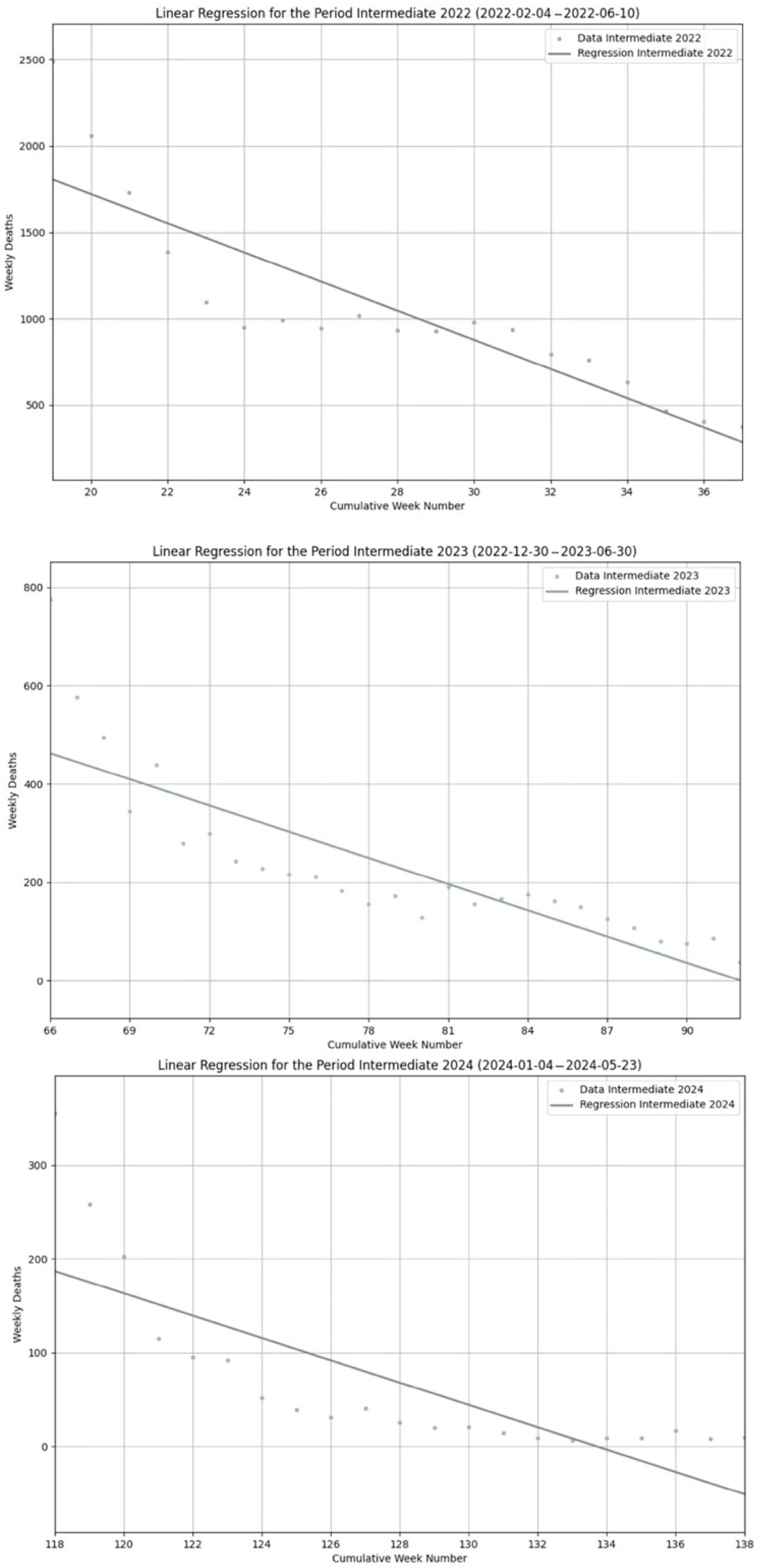
Figure 2 is comprised of three different plots. From top to bottom, the regression segments for Winter 2021, Winter 2022 and Winter 2023. This is similar for Figure 3. From top to bottom: Summer 2022, Summer 2023 and Summer 2024. Finally, Figure 4. From top to bottom: Intermediate 2022, Intermediate 2023 and Intermediate 2024. Each plot reports the dates of the beginning and the end of the considered periods. In all the plots, Y represents the number of weekly COVID-19 deaths for each given week registered along the X axis. Each figure also comes with the values of the parameters β₀, β₁ and R² computed for each single plot, specified in the corresponding captions.

To be clearer, the measurements of the β₁ and R² parameters, per each different season, are also summarized in

Table 2. Characteristics of the regression segments for COVID-19 deaths in Figure 2, Figure 3 and Figure 4: values of β₁ and R² per period, plus average and standard deviation per season.

Period	β1	r2	β1: Average/SD per Type of Season	R2: Average/SD per Type of Season
Winter 21	126.45	0.76	55.75/61.29	0.74/0.05
Winter 22	23.28	0.67	55.75/61.29	0.74/0.05
Winter 23	17.52	0.80	55.75/61.29	0.74/0.05
Summer 22	54.80	0.36	22.90/22.55	0.63/0.05
Summer 23	6.72	0.70	22.90/22.55	0.63/0.05
Summer 24	7.20	0.82	22.90/22.55	0.63/0.05
Inter. 22	−84.38	0.77	−38.01/32.87	0.70/0.19
Inter. 23	−17.76	0.71	−38.01/32.87	0.70/0.19
Inter. 24	−11.89	0.62	−38.01/32.87	0.70/0.19

, along with the average and the standard deviation values, computed per each type of the different seasons under consideration.

As already anticipated, while the slope of a regression segment depicted in a given plot offers a visual impression of the velocity with which the corresponding COVID-19 mortality trend is increasing or decreasing, the numerical value of the associated β₁ parameter provides the exact number by which COVID-19 deaths are progressively increasing with each new week of that period. On the other end, R² informs on how well a given linear regression segment has fitted the available observations (i.e., the initial COVID-19 deaths), on a scale from 0 to 1 (0–100%).

Several facts are noteworthy when examining Figure 2, Figure 3 and Figure 4 and Table 2.

First, we can observe that all the winter periods follow an increasing COVID-19 mortality trend, with positive slopes of the regression segments (Figure 2). Similarly, all the summer periods follow an increasing mortality trend (Figure 3). On the contrary, all the intermediate periods decline along a decreasing trend, with negative slopes of the corresponding regression segments (Figure 4).

Second, the increasing trends of winters and summers are different: the increasing mortality trend of winters is more pronounced, with an average β₁ value of 55.75 versus an average β₁ value for summers of 22.90 (fourth column of Table 2).

Third, there is a high variance of the slope coefficients within similar periods over different years, with a tendency towards less positive/negative slope coefficients with the passage of years.

Take Winters: we begin with a β₁ value of 126.45 for Winter 2021, we proceed with a β₁ value of 23.28 for Winter 2022, and we conclude with a β₁ value of 17.52 for Winter 2023, yielding a SD value for β₁ of 61.29 (second and fourth columns of Table 2). This situation repeats similar during the summer periods, with the following values: Summer 2022 (β₁ = 54.80), Summer 2023 (β₁ = 6.72), Summer 2024 (β₁ = 7.20). The SD value for β₁ is equal to 22.55 (second and fourth columns of Table 2). With intermediate periods, although negative, we observe the slopes becoming progressively less negative going from 2022 to 2024, with an average value of the β₁ coefficient of −38.01 (SD 32.87), and a series of consecutive values (2022–2024) of β_1, which are as follows: −84.38, −17.76, −11.89 (second and fourth columns of Table 2).

Finally, if we consider the three Figure 2, Figure 3 and Figure 4 as a whole, we can observe that the decreasing trends of the COVID-19 mortality, over all the three intermediate periods with their relatively long duration in time, have played the important role of compensating the upward drifts registered during winters and summers, thus contributing to the general declining trend of the COVID-19 mortality registered on the entire period of interest.

Coming to the R² values, they confirm that our segmented linear model has a good fit with the initial COVID-19 deaths data (with just an exception). In fact, the winter periods (third and fifth columns of Table 2) show very good R² values, precisely, Winter 2021 (R² = 0.76), Winter 2022 (R² = 0.67), Winter 2023 (R² = 0.80), with an average value of R² of 0.74 (SD 0.05). This is similar for the intermediate periods (third and fifth columns of Table 2): Intermediate 2022 (R² = 0.77), Intermediate 2023 (R² = 0.71), Intermediate 2024 (R² = 0.62), with an average value of R² of 0.70 (SD 0.06). Something slightly different occurs for summers with the following values (third and fifth columns of Table 2): Summer 2022 (R² = 0.36), Summer 2023 (R² = 0.70), Summer 2024 (R² = 0.82), yielding an average R² value of 0.63 (SD 0.19). Indeed, the low value of R² for Summer 2022 is a consequence of what happened during that season when a rapid ascending trend of COVID-19 deaths was registered, beginning approximately at mid of June 2022, but peaking very soon on July 7, with 1111 deaths, to return to its previous baseline values at mid of August [18]. Unfortunately, the rapid up and down of this summer pandemic wave has hardly a good fit with any linear model. Consequently, the slope of the regression segment, in this specific case, does not reflect well the speedy change from an upward to a downward drift of the COVID-19 mortality profile of those weeks, thus explaining the corresponding low value for R² in this specific case. Regarding our segmented linear regression model, it is also worth noticing that all the p-values computed during the use of our model have been, to a large degree, below the significative value of α = 0.05, thus providing a further confirmation of the plausibility of this analysis.

To conclude this section, we finally report in Figure 5 a comprehensive graphical summary of our results. They consist of the initial time series data of COVID-19 deaths of Figure 1, divided over the nine different seasonal periods of interest, with superimposed the linear regression segments computed by our model and previously presented in Figure 2, Figure 3 and Figure 4.

4. Discussion

Previous studies have demonstrated that strong evidence of a sinusoidal seasonal pattern that repeats over a one-year period cannot be found for the COVID-19 illness, at least in Western countries [10,19,20]. Nonetheless, with the present study, we have demonstrated that both ascending and descending seasonal COVID-19 mortality trends have been observed in Italy over the period from September 2021 to September 2024.

In particular, the positive slopes of the segments of a piecewise linear regression model, fitted with the time series data of COVID-19 deaths of that three-year long period, have revealed the recurrence of ascending COVID-19 mortality trends in all the winters and in the summers of that period, but more pronounced in winters.

Instead, the segments associated with all the three intermediate periods, extending from the end of winters to the beginning of summers, with their negative slopes, have revealed descending mortality trends that have played the role to compensate the upward drifts registered during winters and summers, thus contributing to the general decreasing rate of the COVID-19 mortality.

In the end, these seasonal upward/downward oscillations, repeated for three years, have contributed to going from an average number of weekly deaths from COVID-19 of almost 1000 in the period October 2021–September 2022 to around 100 in the period October 2023–September 2024 [3,4].

All this said, the first limitation of our study is that it has scrutinized COVID-19 deaths data from a very specific time period (September 2021–September 2024). In that period, the epidemiological landscape in Italy was that of when the initial Omicron variant took over and then diversified into multiple post-Omicron sub-variants that gained an extremely increased survival fitness, leading to pandemic waves recurring in different seasons of the same year [21]. While the mathematical approach we have used to derive our findings remains valid, different results could be obtained by examining different pandemic periods with the circulation of different SARS-CoV-2 lineages.

We also recognize that this study has avoided identifying the motivations behind the upward/downward seasonal drifts we have identified. They can be attributable to several, different causes (or even to a combination of them), including (i) climatic and environmental factors, (ii) social behaviors, like dense people gathering during holydays and vacations or common spreading events, (iii) decreasing immunity from previous infections and vaccinations and (iv) various kinds of control and prevention measures. We are aware that further research is necessary to evaluate the role of those triggers and factors in the seasonal variations of mortality from COVID-19 [6].

Nonetheless, while this can be seen as a limitation of our research, we have decided to avoid taking part in the discussion about the causes of the seasonal COVID-19 deaths oscillations, with the precise idea to observe a natural phenomenon only to detect the presence of those seasonal increasing/decreasing mortality trends with neutrality, and regardless of the underlying factors.

We would emphasize again that this choice is deliberate (and methodologically sound). In fact, it should be considered that in the present case this kind of limitation comes from the uncertain nature of the available data, leading to the two following situations, regarding, for example, the role of vaccinations and the number of registered infections.

First, after the post-Omicron variants emerged, there was a noticeable shift in the perceived significance of vaccination, particularly regarding the quantity of doses to be received. While the initial vaccination courses and boosters remained crucial for preventing severe illness, the highly transmissible and immune-evasive nature of the variants circulating in the years of our study has made the population less inclined to get vaccinated, yielding a very considerable reduction in the doses administered in 2023 and 2024 [22].

Second, ever since post-Omicron variants gained prominence, tracking the number of infected people has become an unreliable measure [23]. This is underscored by the high level of caution with which the Italian Authorities have made their decisions based on this particular data in those very recent years.

Writing about the causes of what we have observed and measured (i.e., the seasonal mortality trends of these latest years), without resorting to reliable data, would not help towards an in-depth understanding of this phenomenon. We opted, instead, for an observational approach from which the seasonal mortality trends subject of our findings, were just the fundamental result. Let others explore the possible causes behind the phenomenon we have evidenced; if indeed feasible, it reflects a serious and conscious approach to scientific research.

To be noticed is also the fact that other studies have gone down the road of exploring the digital world as a potentially interesting and alternative source of information regarding the COVID-19 disease [24,25]. We recognize this as an alternative path to follow to discover new associations. Nonetheless, the level of uncertainty inherent in it was neither suitable to be managed with our type of mathematical approach nor compatible with the kind of stable results we were looking for.

Another characteristic of our study has been the decision to resort to a simple linear regression model. We perfectly know that more sophisticated epidemiological models, time series analyses, Poisson and generalized linear models are usually necessary for a more robust and accurate management of COVID-19 data count [26,27,28].

However, it should be clear that the target of our research was not to create a model for a standard count data analysis of COVID-19 deaths [29,30,31]. What we were strongly interested in, indeed, was knowing whether the mortality trends were increasing or decreasing, beyond knowing precisely by how much.

Not only that, but it might seem that with a simple linear regression, we have offered only a superficial look at these mortality trends. This would largely be due to the fact that the strict assumptions for a linear regression to function properly have not been met.

Statistically speaking, this is condensed into the following facts: the errors of the model (or residuals) are not normally distributed and homoscedastic (constant variance), and the number of deaths on a given day may be correlated with those of the preceding days (autocorrelation).

However, faced with this doubt, one should inspect the plots in Figure 1, Figure 2, Figure 3 and Figure 4 more carefully. These show, with the exception of only one: the Summer 2022 case we have already discussed extensively, a situation where the distribution of the residuals does not seem to deviate too much from a normal distribution, with the observed data almost always well-aligned along the interpolating line, and furthermore, the variance does not seem to increase as the mean increases. These hypotheses would be confirmed by Q-Q plots, but for reasons of space, they cannot be presented here.

Finally, on the issue of autocorrelation, it should be given greater weight to the fact that grouping counts weekly (or into longer time intervals) effectively tends to reduce the autocorrelation problem seen in daily data.

In closing this specific issue, it is undisputed that simple linear regression is not generally appropriate for COVID-19 death counts due to its rigid assumptions. Yet, every general rule should be interpreted in the context of the specific case, and this one (as demonstrated by Figure 1, Figure 2, Figure 3 and Figure 4) seems to fit that description perfectly. Furthermore, our linear regression has been particularly useful in providing a clear identification of the COVID-19 mortality trend for each season of interest, helping to compare the slopes of different seasonal mortality profiles, over various years, while showing the seasons to take under more control for the benefit of those who are seasonally vulnerable.

Considering all this, we think that linear regression can be considered sufficiently reliable and adequate in this specific context.

Similar arguments can be offered regarding the issue of the goodness-of-fit of our regression model with respect to the available COVID-19 deaths data. Again, it should be clear that we were not looking for the best-optimized model, but for a set of regression segments able to guarantee an acceptable approximation of the available deaths data, being acceptable any segment with a coefficient of determination above the threshold of 60/65%, as indicated in the specialized literature [32].

On the other end, using a segmented linear regression model has given the advantage of a temporal decomposition of the time series of the COVID-19 deaths data, allowing the differentiation between severe and moderate variations of the COVID-19 deaths trends, while distinguishing seasonal alterations from minimal upward/downward drifts of the time series. To conclude this discussion, we believe that, in our case, these technical limitations have touched more upon the specificity of the investigated topics rather than addressing a weakness of our analysis. Moreover, writing about them should help towards an in-depth understanding of these issues [33,34,35,36,37,38].

Limitations reside, finally, in the use of Italian data. In fact, on the one end, the extension to different geographies could result in different results. On the other end, we used data made available by the Italian Government in the form of aggregated measures from two different sources (Civil Protection Department and Ministry of Health). In several cases, those measures have changed value over time, subject to corrections and adjustments, reaching a relative stability only recently.

5. Conclusions

We have fitted a segmented linear regression model to investigate the occurrence of seasonal variations of COVID-19 mortality trends in the period September 2021–September 2024, when the SARS-CoV-2 Omicron and post-Omicron variants were mostly predominant in Italy. The slopes of the segments of our regression model suggest that, despite a general declining trend of the COVID-19 mortality over the entire period of observation, seasonal increasing variations of deaths from COVID-19 have occurred during all the winters and the summers of the period, but they were more pronounced in winters. Since these increasing seasonal alterations of the COVID-19 mortality have always been compensated by consistent downward drifts occurring during the intermediate periods between winters and summers, they have been considered a cause for concern only occasionally. With our research, we have provided a contribution for the benefit of that subset of at-risk populations who are seasonally vulnerable, having clearly identified the seasons to consider with more attention. However, all this should be understood simply as the observation of a factual finding, without the intent to provide public health recommendations. In doing so, we reaffirm the purely observational nature of this study.

This paper is based on a preliminary, non-peer-reviewed version of this study [39].