Abstract
Graphene interfaces in layered dielectrics can support unique electromagnetic modes, but analyzing these modes requires robust computational techniques. This work presents a numerical method for computing TE-polarized eigenmodes in a planar stratified dielectric slab with an infinitesimally thin graphene sheet at its interface. The governing boundary-value problem is reformulated as coupled initial-value problems and solved via a customized shooting method, enabling accurate calculation of complex propagation constants and field profiles despite the discontinuity at the graphene layer. We demonstrate that the graphene significantly alters the modal spectrum, introducing complex leaky and surface waves with attenuation due to graphene’s conductivity. Numerical results illustrate how the layers’ inhomogeneity and the graphene’s surface conductivity influence mode confinement and loss. These findings confirm the robustness of the proposed computational approach and provide insights relevant to the design and analysis of graphene-based waveguiding devices.
1. Introduction
Graphene-based films and multilayer planar structures have attracted considerable attention due to their exceptional electrical, optical, and mechanical properties [1,2,3,4]. These materials play a central role in emerging applications, including optoelectronic devices, plasmonic components, and integrated waveguide systems.
Electromagnetic wave propagation in graphene-coated geometries has been studied extensively. Of particular interest are cylindrical waveguides coated with graphene, where various modal phenomena—such as TE and TM modes, complex (leaky or trapped) surface waves, and hybrid plasmonic modes—have been investigated in detail (see [5,6,7] and references therein).
Among such configurations, multilayer sandwich-type structures, such as dielectric–graphene–dielectric and graphene–dielectric–graphene systems, have revealed a wide range of tunable wave phenomena [8]. Notably, these structures support hybrid surface waves whose properties can be controlled via external magnetic fields, and enable the coupling of TE and TM modes under magneto-optical effects [9,10].
Despite the growing body of numerical results, a rigorous mathematical framework for wave propagation in stratified media containing graphene interfaces remains insufficiently developed [10]. In contrast to conventional homogeneous or inhomogeneous dielectric layers, the presence of an infinitesimally thin graphene sheet requires interface conditions involving discontinuities, effective surface conductivities, and possibly dispersive or nonlinear effects. Moreover, the combined modeling of electromagnetic and mechanical interactions introduces further complications [2,10,11].
A common shortcoming in the existing literature (e.g., [5]) is the lack of well-posed mathematical formulations, including the absence of spectral theory tools to justify the existence and nature of normal modes in the complex propagation constant domain.
The present work addresses these gaps by formulating and solving a model problem for a two-layer planar structure with an embedded graphene interface. Our objective is to develop a mathematically consistent and numerically tractable framework that captures the essential spectral features of the system.
Building on our previous research on open metal–dielectric waveguides with circular and planar symmetry [12], we employ a numerical-analytical approach based on the reduction to ordinary differential equations and the use of initial-value formulations. This methodology enables the classification and computation of surface, leaky, and complex modes with high accuracy.
In this paper, we adapt and extend this technique to planar stratified media with graphene layers. The resulting framework provides both qualitative insight and quantitative results regarding the modal spectrum, field profiles, and the role of interfacial conductivity in shaping wave behavior.
2. Statement of the Problem
We consider the three-dimensional Euclidean space equipped with a Cartesian coordinate system and filled with a homogeneous, isotropic, and source-free exterior medium characterized by vacuum permittivity and permeability .
The structure under consideration is a planar waveguide occupying the spatial region
which is bounded in the transverse direction x and unbounded in the y- and z-directions.
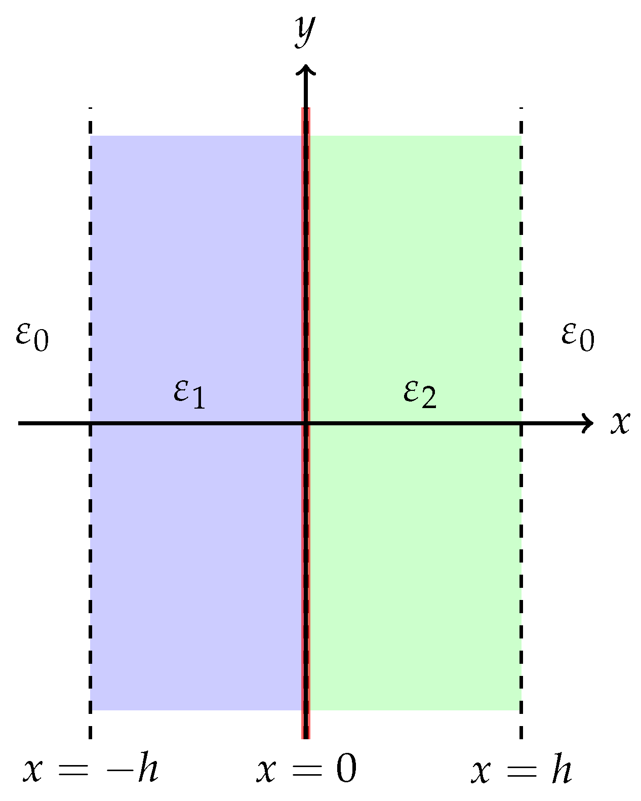
The waveguide consists of two adjacent inhomogeneous layers of thickness h, separated by an infinitesimally thin graphene sheet located at the central interface (see Figure 1). The surrounding medium for is assumed to have constant permittivity . The relative permittivity functions within the layers are denoted by for and for .
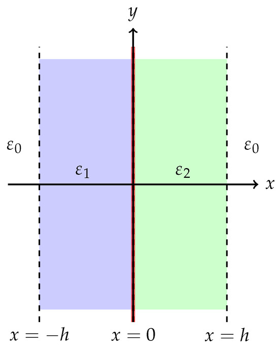
Figure 1.
Cross-sectional view of the stratified waveguide structure. The interior consists of two dielectric layers with spatially varying permittivities (left, blue) and (right, green), separated by an infinitesimally thin graphene interface (red) located at . The outer regions and are occupied by a homogeneous background medium with constant permittivity .
We assume harmonic time dependence of the fields of the form , where denotes the angular frequency. The analysis is focused on determining the modal structure and propagation characteristics of electromagnetic waves supported by the waveguide, including the effects introduced by the presence of the graphene interface.
The goal is to analyze the spectral properties of this structure and identify the modal solutions supported by the layered configuration, with particular emphasis on how the graphene interface affects mode confinement and radiation. We assume that the relative permittivity distribution in the entire space is defined as
where, denotes the constant relative permittivity of the exterior medium (typically vacuum), while and represent the relative permittivities of the inner dielectric layers, defined on the intervals and , respectively. These functions represent spatially varying relative permittivities, i.e., dimensionless dielectric functions normalized by the vacuum permittivity . This convention is standard in electromagnetic modeling and will be used throughout the paper.
In the present study, we allow and to be arbitrary continuous complex-valued functions. This general framework enables us to explore several physically relevant cases:
- Conventional dielectrics: are real-valued and strictly positive, corresponding to non-absorbing media with wave-confining properties;
- Metamaterial-type regimes: take real negative values over some subintervals, allowing for anomalous dispersion and surface plasmon effects;
- Absorbing media: are complex-valued with , accounting for material losses within the layers.
This flexibility in the choice of allows us to investigate both standard and exotic propagation scenarios, including surface wave localization, leaky behavior, and modal attenuation due to absorption.
To study TE-polarized waves in this structure, we seek nontrivial time-harmonic solutions to the source-free Maxwell system
where is the angular frequency and is the magnetic permeability of vacuum.
Due to translational invariance along the z-axis, we consider wave solutions propagating in the z-direction with a complex propagation constant , i.e., solutions of the form
Substitution into (1) yields a second-order differential equation for the transverse electric field component in each region, together with expressions for the magnetic field components and in terms of and its derivatives.
The presence of material interfaces at , , and introduces transmission conditions for the tangential components of the fields. These conditions take the form
where is the (complex-valued, possibly frequency-dependent) surface conductivity of the graphene film, and the jump operator is defined as
In this formulation, the jump in the magnetic field across the graphene sheet reflects the surface current induced by the tangential electric field, according to the standard interface model for infinitely thin conducting layers.
Importantly, we do not impose a radiation condition as , since we aim to characterize the full spectrum of possible values of , including both surface and leaky modes. This choice allows us to treat the problem as a spectral (eigenvalue) problem with respect to the complex-valued propagation constant .
By substituting the harmonic ansatz for the fields (2) into Maxwell’s system (1), we obtain the following expanded system of ordinary differential equations:
where prime notation denotes differentiation with respect to x.
From the second and third equations in (6), we can explicitly express the components of the magnetic field in terms of the tangential electric field component :
It follows from Equation (7) that the entire electromagnetic field of a TE-polarized mode can be reconstructed from a single scalar function
Accordingly, the problem reduces to determining the tangential component of the electric field .
Substituting expressions (7) into the first equation of system (6), we arrive at the following second-order ordinary differential equation for :
This equation holds in each subdomain where is continuous. The coupling between the subdomains is governed by the transmission conditions (3)–(5), which encode the continuity of the tangential electric field and the appropriate jump in the magnetic field due to the surface conductivity of the graphene interface. The transmission conditions are as follows:
where the jump notation indicates the limit from the left/right of the interface, and
is a dimensionless parameter that quantifies the strength of electromagnetic coupling across the graphene sheet due to its surface conductivity.
Thus, the spectral problem consists in finding all complex values of for which the boundary value problem (8)–(11) admits nontrivial solutions in the appropriate functional class.
In the regions and , the relative permittivity takes the constant value . Substituting this into Equation (8), we obtain the second-order differential equation
where we introduce the auxiliary (generally complex) spectral parameter
which characterizes the effective transverse behavior of the field in the homogeneous outer regions and facilitates the classification of wave types.
In the region , we choose the solution of Equation (12) in the form
where A is an arbitrary constant.
Similarly, for the same Equation (12) holds, and we represent its solution as
where is an independent constant.
In the interval , the relative permittivity is given by the function . Substituting this into Equation (8), we obtain the equation
where
In the region , where , we analogously obtain the equation
with
Definition 1.
A complex number is called a propagation constant of the problem if there exists a nontrivial scalar function satisfying the following conditions:
- in the interior regions and , satisfies the differential equations
- the function satisfies the transmission conditions (9)–(11) at the interfaces , , and .
Definition 2.
A propagating wave corresponds to the case where the spectral parameter λ is a real number, . In this case, the wave solution exhibits sinusoidal oscillations in the transverse direction without exponential growth or decay. Physically, this describes a wave that transports energy laterally across the structure without attenuation in space.
Definition 3.
An evanescent wave is characterized by a purely imaginary spectral parameter, , i.e., with . The corresponding field decays exponentially in the transverse direction. Evanescent waves do not carry energy across the medium but are spatially localized near the core of the structure. They typically appear in total internal reflection or near-field regimes.
Definition 4.
A complex wave corresponds to a spectral parameter with both nonzero real and imaginary parts: and . These waves combine both oscillatory and exponentially growing or decaying behavior in space. Complex waves arise in lossy media, open waveguides, or leaky configurations where energy can radiate away from the core region.
Definition 5.
A wave is called a surface wave if the corresponding field profile satisfies the condition
That is, the amplitude of the wave decays in both transverse directions away from the core region. Surface waves are strongly localized near the interface and are of particular interest in layered or plasmonic structures, where field confinement is critical.
Definition 6.
A wave is called a leaky wave if the field profile satisfies
This behavior corresponds to energy escaping from the core of the structure into the surrounding space. Leaky waves are commonly encountered in open waveguide systems and resonant radiating structures.
Figure 2 provides a visual summary of this classification in the complex -plane.
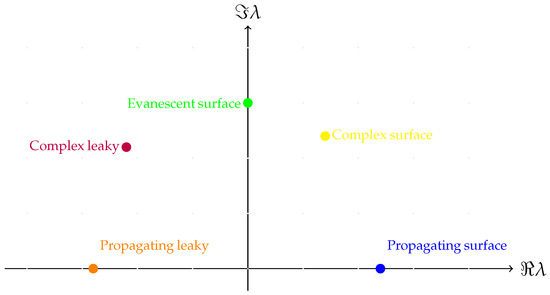
Figure 2.
Classification of wave types in the complex -plane. The horizontal and vertical axes correspond to and , respectively. Each colored point represents a distinct wave type as defined in Definitions 2–6.
The original spectral parameter of the problem is the longitudinal propagation constant , which appears in the field ansatz and governs the behavior of the solution along the z-axis. The quantity is the eigenvalue in the formulation of the spectral problem for the Maxwell system.
Although serves as the primary spectral parameter governing longitudinal behavior, the transverse profile of the field—and, consequently, the classification of wave types—is fully determined by the auxiliary quantity . This distinction is essential: surface and leaky waves are defined by their asymptotic decay or growth in the transverse direction, which is dictated by , not . Therefore, it is customary and natural to express modal classifications in terms of , especially in open or lossy waveguides.
3. Numerical Method
To compute the complex eigenvalues of the problem defined in Section 2, we employ a numerical procedure based on the shooting method. This classical approach reduces the boundary-value spectral problem to a system of initial-value problems (Cauchy problems) integrated across the domain, with continuity and interface conditions enforced at internal boundaries. In essence, the shooting method constructs solutions on each layer of the structure and adjusts the spectral parameter until the desired matching conditions are satisfied at the outer interface. This yields a nonlinear dispersion equation , whose roots correspond to the propagation constants of the supported modes.
To implement this idea for a stratified geometry with an embedded graphene interface, we proceed as follows.
We begin by considering the Cauchy problem for the second-order differential equation
with the initial conditions imposed at the left interface :
Here, A is an arbitrary nonzero constant (typically set to without loss of generality), and is a complex-valued spectral parameter. The form of the initial derivative reflects the expected exponential behavior in the homogeneous region .
We assume that the Cauchy problem defined by (19) and (20) is globally and uniquely solvable on the segment for a given profile , and that the values and depend continuously on .
Next, we apply the transmission condition at the interface (corresponding to the location of the graphene sheet):
where is the effective interface parameter introduced earlier.
These values serve as initial conditions for the next segment. We consider the Cauchy problem on :
with initial data at given by
Again, we assume that the Cauchy problem (21) and (22) is globally and uniquely solvable for , and that the values and depend continuously on .
To complete the construction, we apply the transmission condition at the final interface :
We now require that the field in the region matches an exponentially decaying solution described in (14). This matching condition leads to the dispersion relation
This equation ensures compatibility with the field behavior in the right homogeneous region and defines the spectrum of the problem.
To determine the complex propagation constants that satisfy the dispersion relation , we numerically solve the equivalent system of real equations
where are the real and imaginary parts of the spectral parameter. Each of these equations defines a level curve in the two-dimensional parameter plane , and the solution to the original dispersion problem corresponds to the intersection points of the zero-level curves and .
To localize these intersections, we discretize a rectangular region in the -plane by constructing a uniform grid. Let
At each grid node , we define the complex number and compute the value of the dispersion function:
Separating real and imaginary parts, we obtain:
To detect the zero-level curves, we analyze the sign changes of the functions and along the horizontal and vertical lines of the grid. For instance, if two adjacent nodes satisfy
then, by the continuity of with respect to , there exists a point such that . This indicates that the node lies close to the curve . Repeating this procedure over the entire grid produces a set of points that approximate the zero-level curve of .
A similar procedure is applied to detect sign changes in and thus to construct an approximate zero-level curve of .
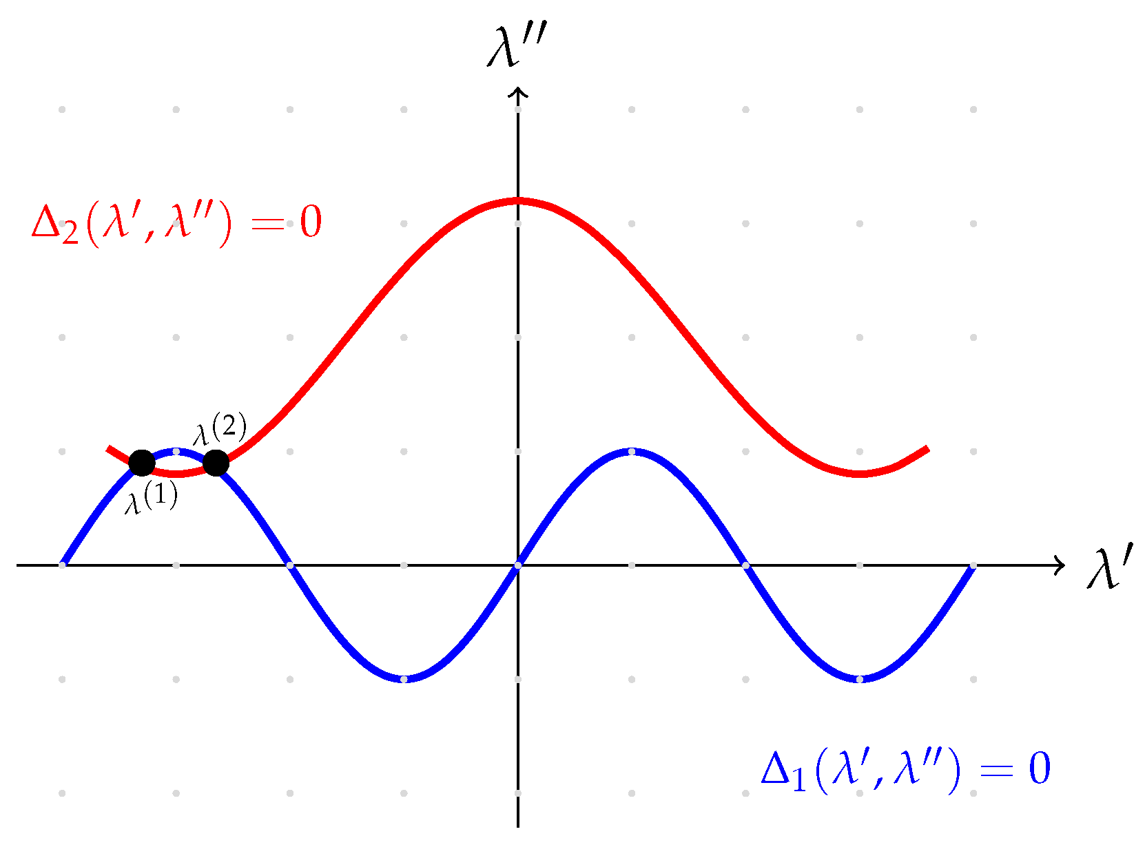
The intersection points of the two curves provide approximate solutions of the system (24), i.e., approximate complex eigenvalues of the spectral problem. A schematic illustration of this procedure is shown in Figure 3. The blue and red curves represent the zero-level sets of and , respectively, and their intersection points correspond to approximate solutions of the dispersion equation. The accuracy of these solutions can be improved by refining the grid, i.e., decreasing the step sizes and .
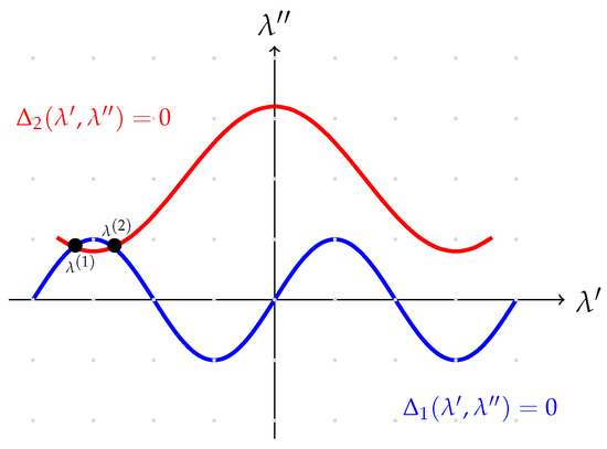
Figure 3.
Schematic illustration of the numerical procedure for solving the system (24). The zero-level curves (blue) and (red) intersect at the points and , which correspond to approximate eigenvalues of the problem.
This method of zero-crossing detection provides a simple and robust means of localizing eigenvalues, especially in cases where derivative-based root-finding algorithms are sensitive to initial guesses or prone to converge to spurious roots. Once intersection points are identified, they can be used as initial approximations for more accurate root-polishing using Newton-like methods or contour tracking techniques.
4. Numerical Results
This section presents a series of numerical experiments aimed at investigating the spectral properties of the stratified waveguide structure described in Section 3. We consider three physically distinct scenarios—conventional dielectrics, metamaterial-type media, and absorbing layers—each characterized by specific choices of spatial permittivity profiles. For each configuration, we compute the complex propagation constants at selected frequencies and reconstruct the associated field distributions .
4.1. Problem Setup and Parameters
We consider a symmetric planar waveguide of total width , with fixed throughout all computations. The outer regions and are occupied by a homogeneous background medium with constant relative permittivity , and the magnetic permeability is set to throughout the entire domain. All quantities in the numerical examples are considered dimensionless, following standard nondimensionalization techniques to simplify the parameter space and interpretation.
The internal structure consists of two adjacent layers of thickness h, characterized by spatially varying permittivity functions for and for , separated by an infinitesimally thin graphene interface at . The graphene sheet is modeled via a surface conductivity parameter , incorporated into the transmission conditions through the dimensionless quantity . In all computations, we set . This value corresponds to a moderate interfacial conductivity and ensures observable yet physically reasonable coupling effects at the interface. The impact of surface conductivity on modal confinement and attenuation has been qualitatively analyzed in earlier studies (e.g., [5]).
Wave propagation is investigated at four representative angular frequencies:
At each frequency, we compute the spectrum of complex propagation constants that satisfy the dispersion relation . The computation is performed over a rectangular grid in the complex -plane with the following discretization:
The dispersion function is evaluated numerically at each node of the grid, and the zero-level curves of and are plotted to detect approximate intersections, which indicate candidate eigenvalues.
For the selected frequency , the approximate intersection points are further refined using a local root-finding method. Specifically, we apply a two-dimensional minimization algorithm to identify nearby values of where attains a local minimum. This procedure enables subgrid-level accuracy in determining complex roots of the dispersion function.
The refined values of are subsequently used to reconstruct electric field profiles , providing detailed insight into the spatial structure of each supported mode.
4.2. Test Case 0: Limiting Behavior as
In this section, we investigate the limiting behavior of electromagnetic modes in a planar stratified structure as the graphene conductivity approaches zero. To this end, we compare two scenarios:
- An analytically solvable configuration: a single homogeneous dielectric slab of width and constant permittivity ;
- A numerically solved configuration: two homogeneous dielectric layers separated by a graphene interface at , modeled by a jump condition depending on .
As , the graphene interface becomes transparent, and the composite structure effectively behaves as a single slab. Therefore, we expect that the roots of the nonlinear dispersion relation for the graphene-coupled problem should converge to the solutions of the linear problem without graphene. This comparison serves both as a validation of the numerical procedure and a physical consistency check.
As a baseline for comparison, we consider a dielectric slab with constant permittivity and no graphene interface. The structure is symmetric about , occupying the interval . We seek nontrivial solutions of the wave equation:
that decay exponentially as . The general solution in the three regions is given by:
Enforcing continuity of u and at yields the following transcendental equation for :
This dispersion relation will serve as a reference for analyzing the limiting behavior of the graphene-modified configuration as the conductivity parameter .
The roots of the analytical dispersion relation for a symmetric dielectric slab with constant permittivity and half-thickness are summarized in Table 1. This configuration admits both complex-conjugate roots corresponding to leaky modes and real-valued roots corresponding to guided surface modes. The table lists initial estimates, refined numerical values, and the physical interpretation of each root.

Table 1.
Roots of the analytical dispersion relation for a symmetric dielectric slab with and .
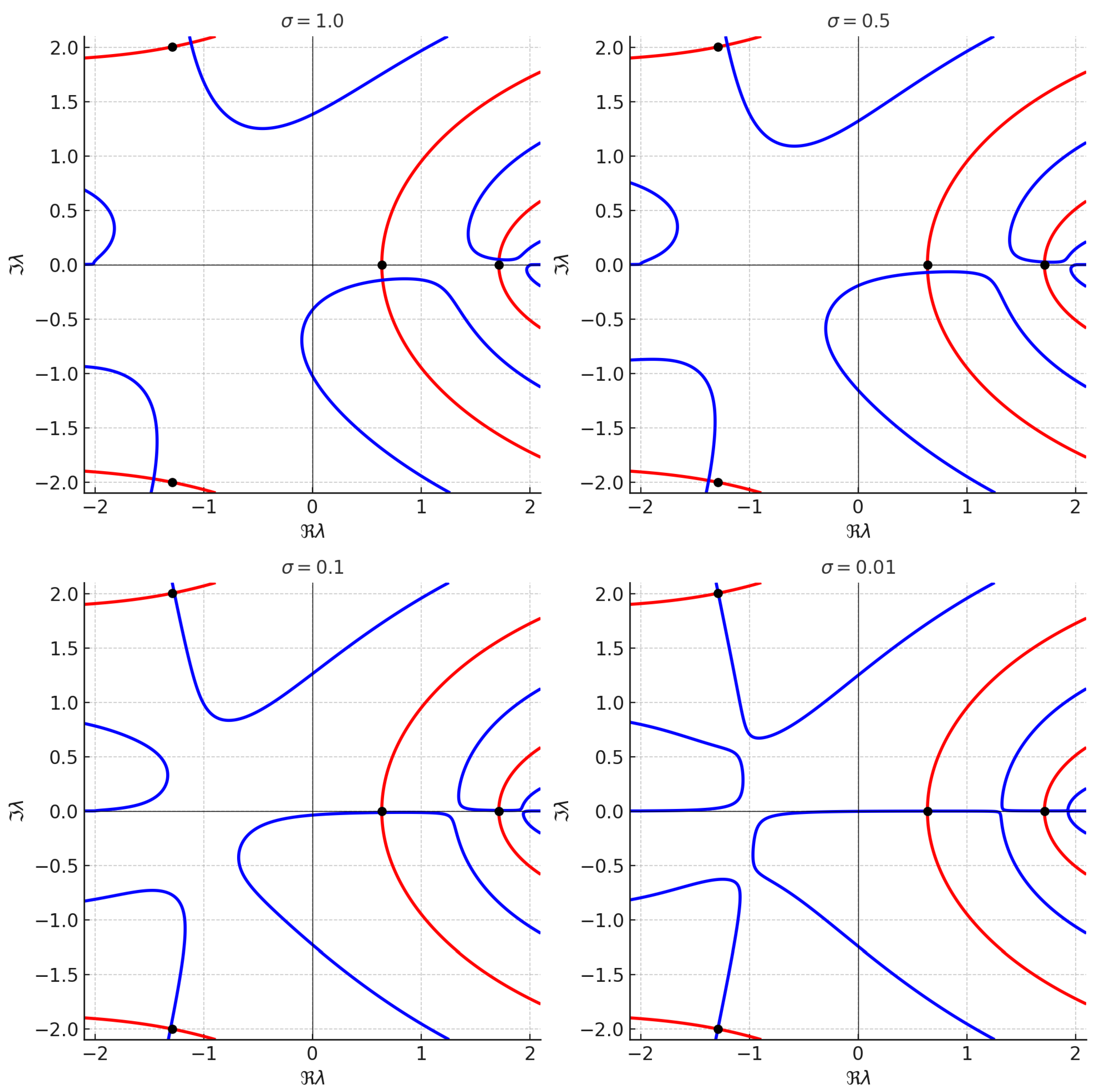
To assess convergence, we repeat the numerical computation for the same geometry but with nonzero graphene conductivity , solving the full nonlinear problem. The frequency is fixed at . The results are visualized in Figure 4, where zero-level contours of the real and imaginary parts of the dispersion function are shown for each . The analytic eigenvalues from Table 1 are superimposed as black dots.
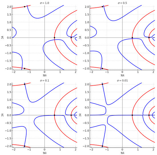
Figure 4.
Computed spectrum of complex propagation constants for the symmetric dielectric slab with constant permittivity and various values of graphene conductivity , , , and . The zero-level contours of (red) and (blue) are shown in the complex -plane. Black dots indicate the analytic roots for the reference case . As decreases, the numerical roots approach the analytic values, confirming the validity of the method.
The convergence of the numerically computed roots toward the analytic values as confirms the correctness of the implementation and serves as a validation of the proposed method.
4.3. Test Case 1: Conventional Dielectrics
In this configuration, both internal layers of the waveguide are modeled as conventional dielectric materials with smooth spatial inhomogeneity. The relative permittivity profiles are chosen as follows:
These profiles ensure that throughout the slab, corresponding to non-dispersive, non-absorbing dielectric media with moderate variation in refractive index.
The goal of this experiment is to determine the spectrum of complex propagation constants for each frequency and classify the resulting wave modes into propagating, evanescent, surface, or leaky types, based on their position in the complex -plane and asymptotic behavior.
The dispersion relation is solved numerically via the method described in Section 3, using a uniform grid in the complex -plane and locating intersections of zero-level curves of the real and imaginary parts of the dispersion function . The resulting mode spectrum is illustrated in Figure 5.
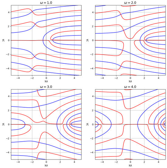
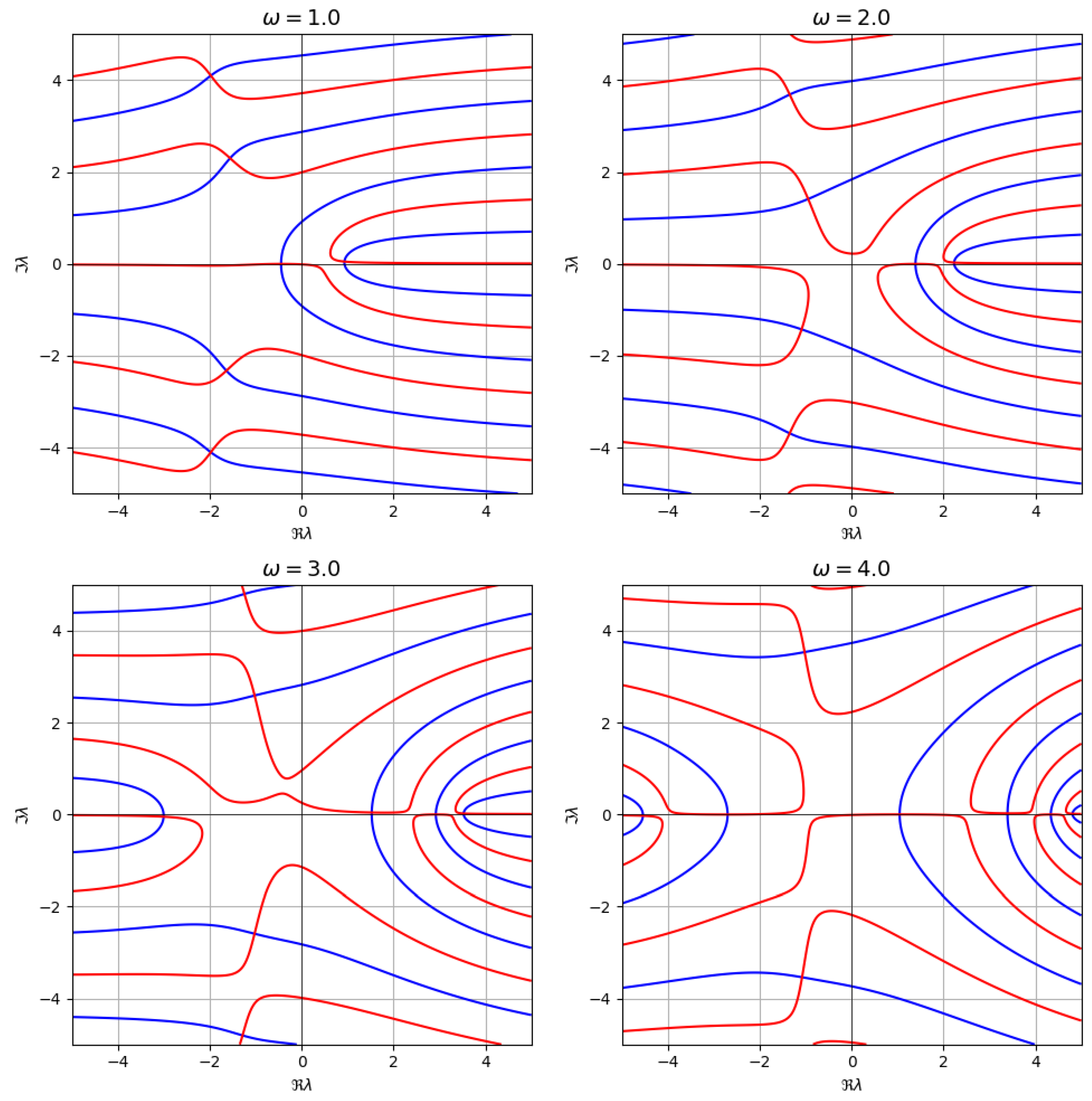
Figure 5.
Computed spectrum of complex propagation constants for the dielectric case at four frequencies . The zero-level contours of (red) and (blue) reveal modal branches and their interaction.
At the reference frequency , several intersection points of the level curves are detected, corresponding to approximate solutions of . These initial estimates are subsequently refined using a local root-finding algorithm. The resulting propagation constants are summarized in Table 2, including both leaky and surface-type modes.
Table 2.
Numerically computed roots of the dispersion relation at .
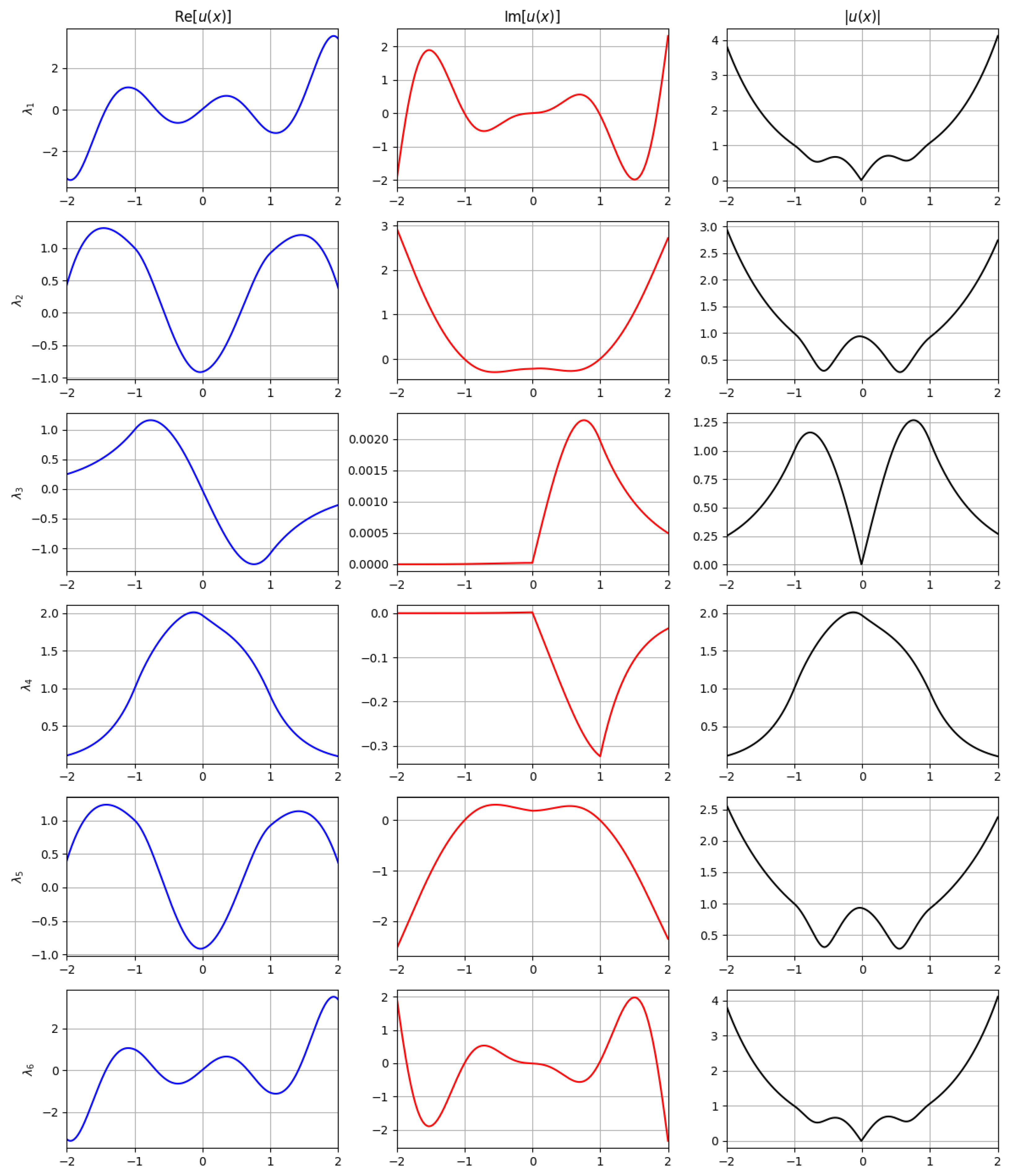
At the reference frequency , the computed spectrum reveals the presence of two distinct types of modes: complex leaky modes and surface modes. No purely propagating or evanescent modes are observed. The refined propagation constants for this configuration are summarized in table. Among them, four eigenvalues (, , , ) appear as complex-conjugate pairs with significant imaginary components. These are interpreted as complex leaky modes, exhibiting both oscillatory and exponentially growing behavior in the transverse direction, consistent with energy leakage into the surrounding medium. In contrast, two eigenvalues (, ) have negligible imaginary parts and are strictly localized. These correspond to surface modes. Specifically, represents a fundamental surface mode with strong confinement near the waveguide core, while is a higher-order surface mode characterized by weak oscillations and broader spatial extent. Overall, the dielectric case demonstrates a balanced spectrum that includes both confined and radiative components, with clear separation between leaky and surface behaviors in the complex -plane.
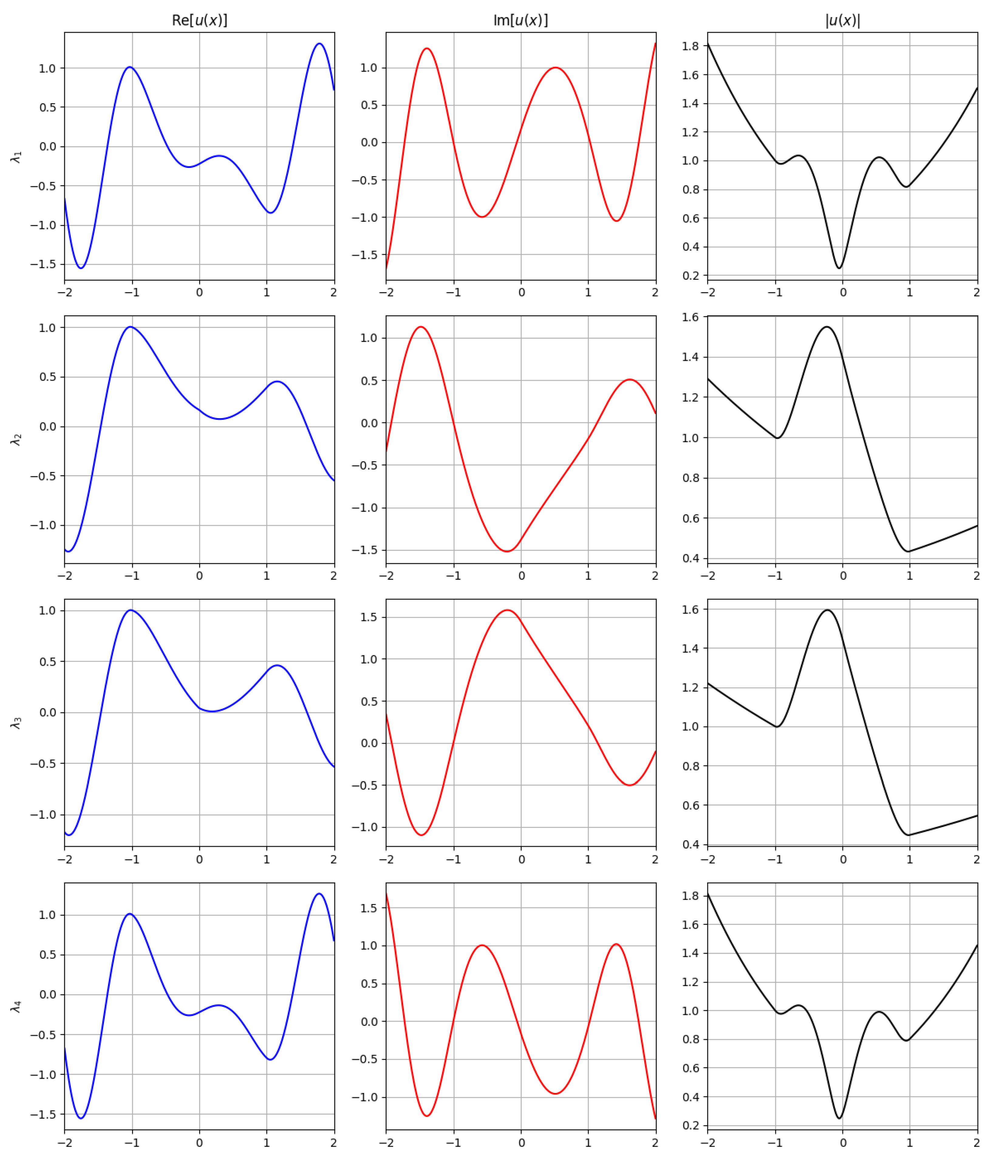
These refined values are used in the subsequent computation of the electric field profiles , discussed below. The resulting modal fields are illustrated in Figure 6.
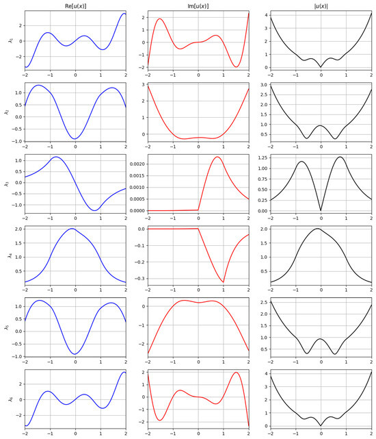
Figure 6.
Electric field distributions at for the conventional dielectric configuration. Each row corresponds to a different mode identified from the spectrum. The plots show the real part (left), imaginary part (center), and magnitude (right) of the electric field.
4.4. Test Case 2: Metamaterial Regime
In this configuration, the permittivity profiles within the slab include regions with negative real parts, modeling an epsilon-negative (plasmonic) response. The functions are defined as follows:
This setup allows for the study of plasmon-like and anomalous dispersion phenomena arising from the presence of negative-index material components.
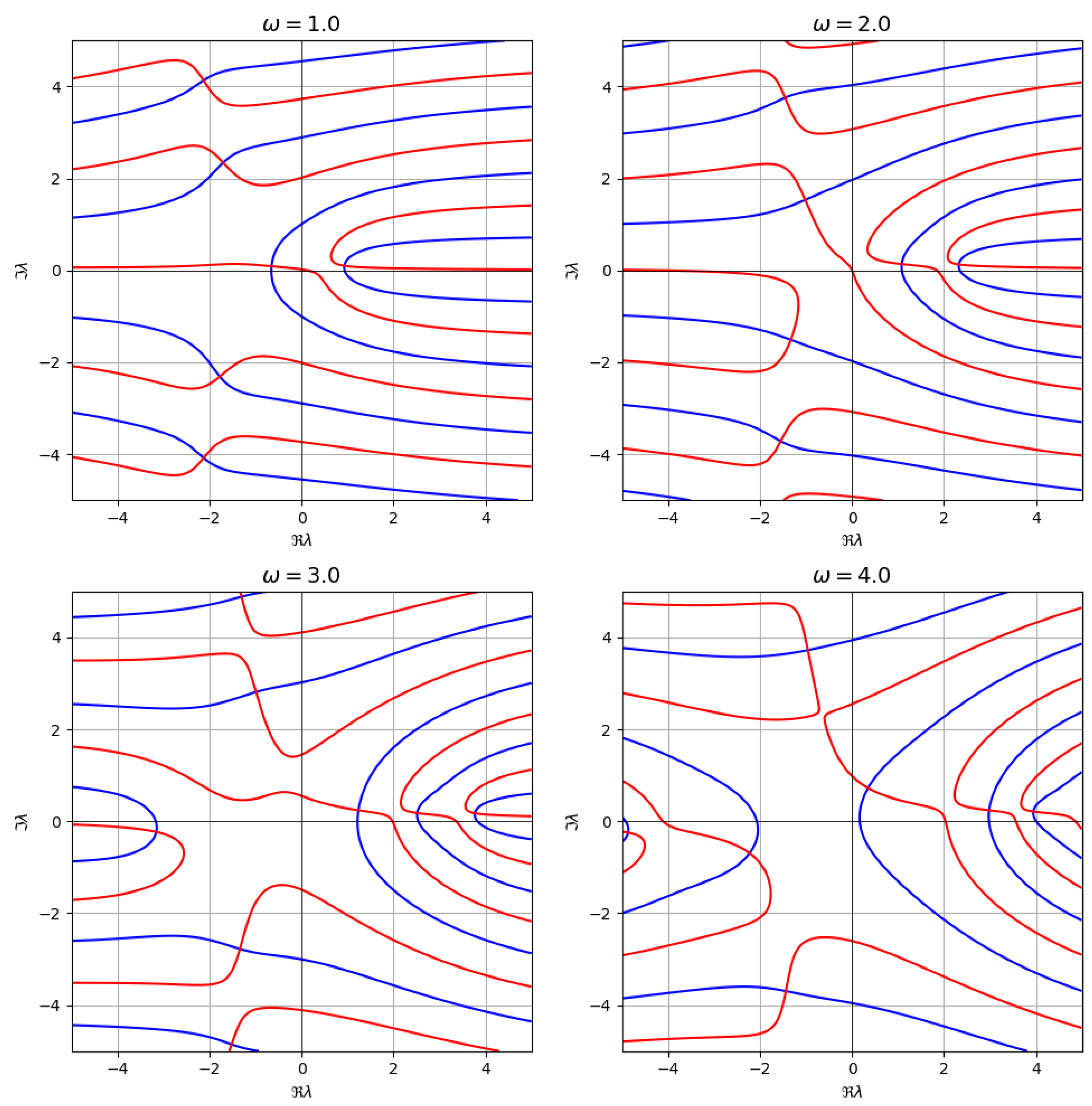
As in the previous case, the dispersion equation is solved numerically on a uniform complex grid at , with propagation constants identified via intersections of and level curves (see Figure 7).
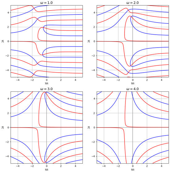
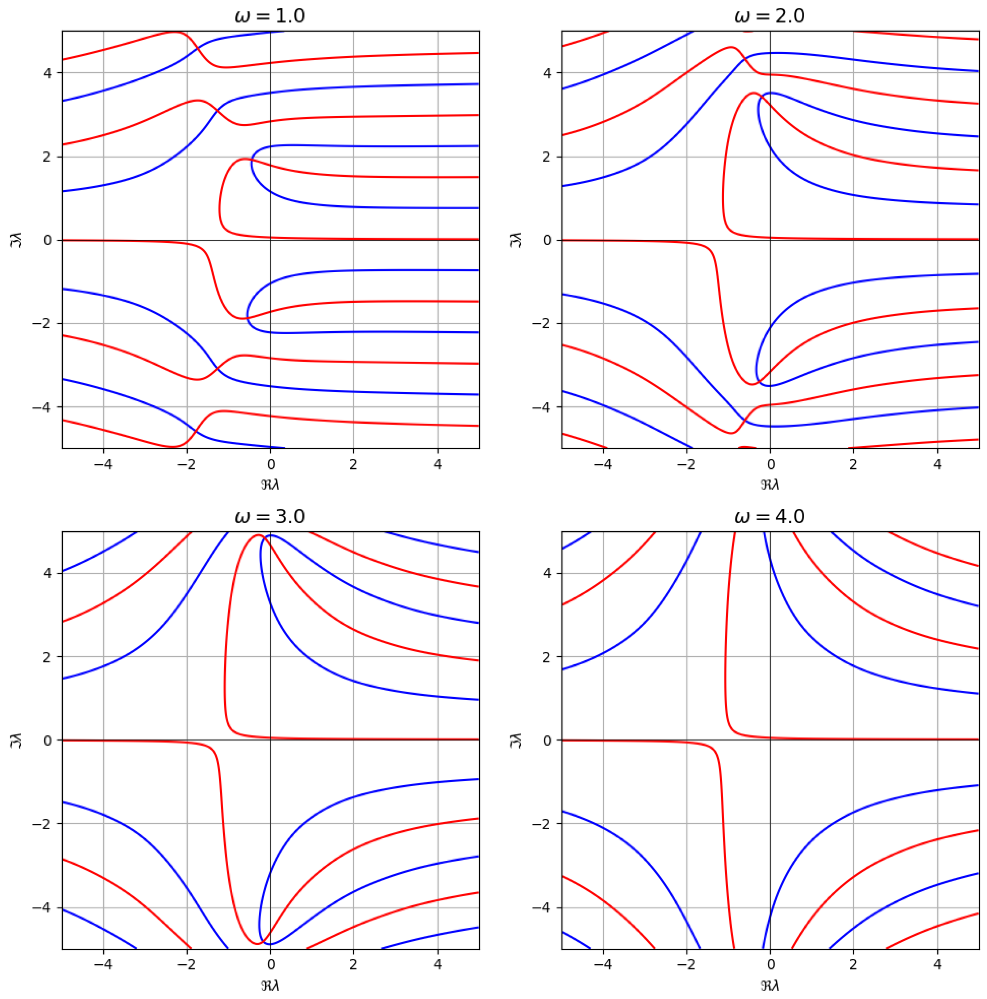
Figure 7.
Spectrum of complex propagation constants for the metamaterial regime. The plots show the zero-level curves of (red) and (blue) for four frequencies.
At the reference frequency , the numerical solver detects several roots of the dispersion relation, including complex-valued solutions with significant imaginary components. These correspond to leaky modes. The computed propagation constants are summarized in Table 3.
Table 3.
Numerically computed complex propagation constants (leaky modes) at .
At , the metamaterial configuration supports only complex leaky modes, with no surface or confined solutions. The eigenvalues form complex-conjugate pairs with substantial real and imaginary parts, reflecting oscillatory, radiative behavior.
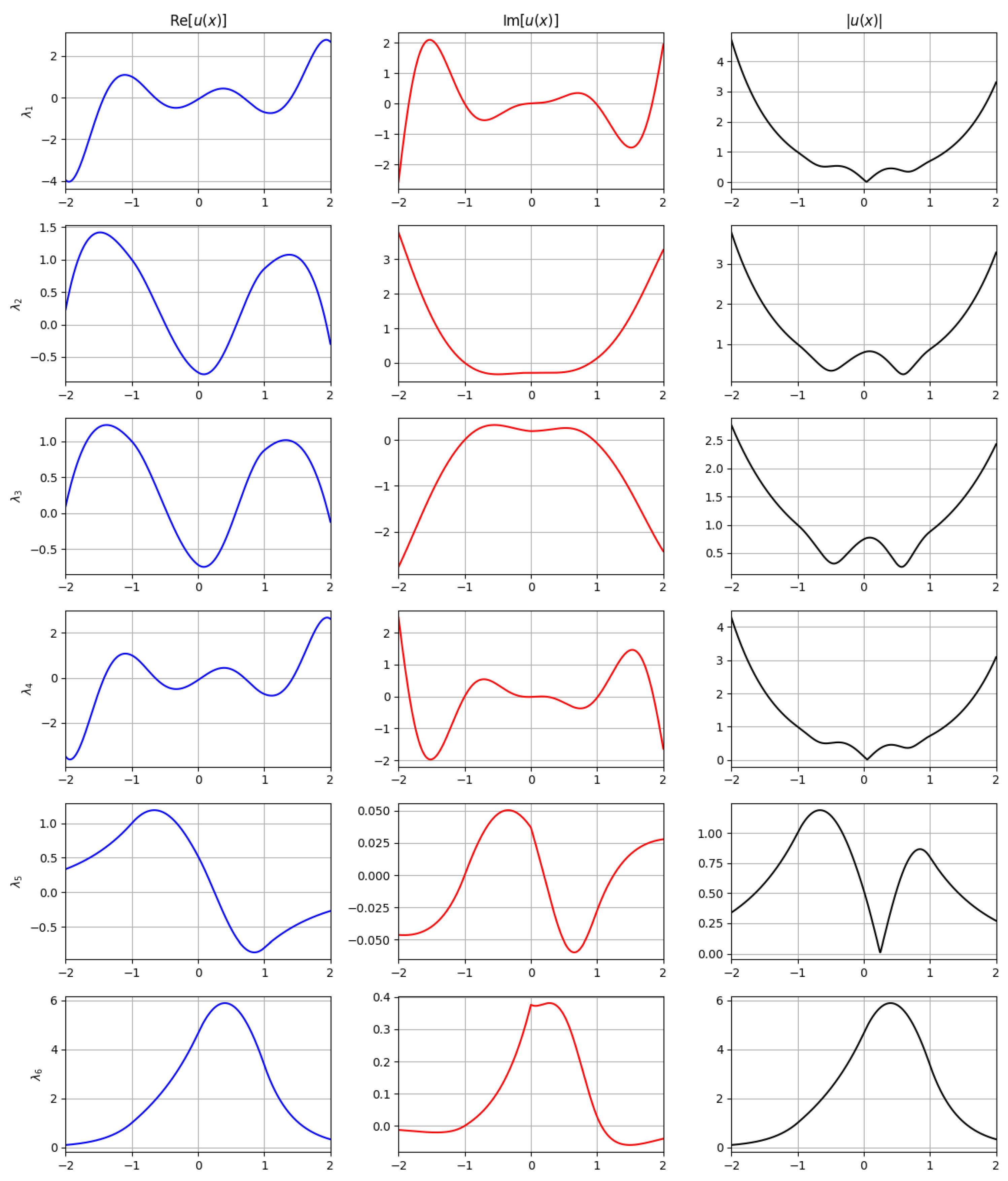
These refined values are used in the subsequent computation of the electric field profiles , discussed below. The field distributions for the metamaterial case are shown in Figure 8.
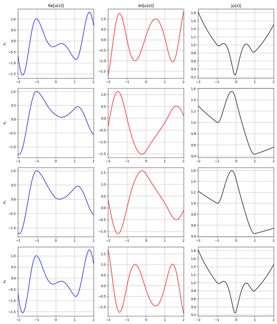
Figure 8.
Computed electric field profiles for the metamaterial regime at . Each row corresponds to a distinct mode, showing the real part, imaginary part, and modulus of the electric field.
4.5. Test Case 3: Absorbing Media
In this configuration, we model wave propagation in a layered structure with material losses. The relative permittivity functions are chosen to be complex-valued with positive imaginary parts, representing weakly absorbing media:
This setup enables us to investigate how material absorption affects mode structure and propagation constants.
The dispersion equation is solved as before; results are shown in Figure 9.
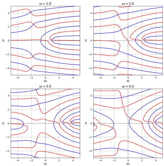
Figure 9.
Complex propagation constants for the absorbing case at four frequencies. The red and blue contours correspond to the zero-level sets of and , respectively.
At the reference frequency , several roots are identified and refined numerically. Due to the presence of absorption, all roots have nonzero imaginary parts, and many exhibit moderate damping in both spatial directions.
In particular, the surface-type modes—which would be purely real or evanescent in a lossless structure—now possess complex-valued propagation constants due to material damping. These modes remain localized near the graphene interface but exhibit attenuation as they propagate transversely. We refer to them as complex surface waves. Other modes exhibit exponential growth in one direction and are classified as complex leaky waves.
The refined eigenvalues and their modal classification are summarized in Table 4. Both complex leaky and surface-type modes are identified based on the imaginary part of the propagation constant.
Table 4.
Refined propagation constants and modal classification at .
To visualize the spatial structure of the corresponding modes, we reconstruct the electric field profiles for each refined at . As expected, even surface-like modes now exhibit slight attenuation in space due to material absorption. These profiles are shown in Figure 10.
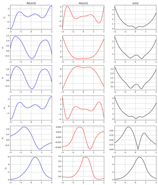
Figure 10.
Electric field distributions at for the absorbing medium configuration. All modes show damping effects due to material losses.
5. Conclusions
5.1. Methodology
We developed a numerical framework to analyze electromagnetic wave propagation in stratified dielectric slabs incorporating an infinitesimally thin graphene interface. The problem was formulated as a spectral boundary-value problem for a second-order differential equation with jump conditions reflecting the graphene’s surface conductivity. A customized shooting method was employed to solve auxiliary initial-value problems and reconstruct the field profiles. The complex dispersion relation was resolved by detecting intersection points of the zero-level contours of and over a discrete complex grid.
5.2. Key Findings
Our computations reveal a rich modal structure across all examined configurations, including:
- Complex surface waves localized near the core but exhibiting transverse damping;
- Complex leaky waves characterized by exponential growth away from the guiding region;
- No purely real (propagating) or purely imaginary (evanescent) modes were observed;
- Modal spectra are highly sensitive to the permittivity profile and the graphene interface.
5.3. Comparative Analysis
We evaluated three physically distinct scenarios:
- Dielectric slabs: A combination of surface and complex leaky modes was observed;
- Metamaterials: Exclusively complex leaky modes dominate due to negative ;
- Absorbing media: All modes are damped, and even surface-type solutions acquire imaginary parts.
These findings confirm the versatility of the method and underscore the importance of full-wave modeling in layered nanophotonics.
5.4. Future Directions
Further developments may include:
- Extension to TM and hybrid polarization states;
- Use of dispersive models for graphene conductivity;
- Investigation of periodic and multi-interface structures;
- Incorporation of time-domain and nonlinear effects;
- Benchmarking against full-wave 3D simulations and experimental setups;
5.5. Practical Implications
The proposed method provides accurate insight into the spectral and spatial behavior of guided and radiative modes in graphene-enhanced dielectric structures. Applications include:
- Graphene-based THz and IR photonic components;
- Plasmonic and leaky-wave sensors;
- Tunable and compact optical modulators;
- Waveguide absorbers and radiation control in layered media.
Our results facilitate the design of next-generation optoelectronic and plasmonic devices by linking material composition to modal behavior.
Funding
This research received no external funding.
Data Availability Statement
No new data were created or analyzed in this study. Data sharing is not applicable to this article.
Conflicts of Interest
The authors declare no conflict of interest.
References
- Guo, S.; Chen, J.; Zhang, Y.; Liu, J. Graphene-Based Films: Fabrication, Interfacial Modification, and Applications. Nanomaterials 2021, 11, 2539. [Google Scholar] [CrossRef] [PubMed] [PubMed Central]
- Liu, Z.; Zhang, X.; Yan, X.; Chen, Y.; Tian, J. Nonlinear optical properties of graphene-based materials. Chin. Sci. Bull. 2012, 57, 2971–2982. [Google Scholar] [CrossRef]
- Rozzi, T.; Mencarelli, D.; Pierantoni, L. Towards a unified approach to electromagnetic fields and quantum currents from Dirac spinors. IEEE Trans. Microw. Theory Tech. 2011, 59, 2587–2594. [Google Scholar] [CrossRef]
- Marconcini, P.; Macucci, M. Transport simulation of graphene devices with a generic potential in the presence of an orthogonal magnetic field. Nanomaterials 2022, 12, 1087. [Google Scholar] [CrossRef] [PubMed]
- Heydari, M.B.; Samiei, M.H.V. Plasmonic Graphene Waveguides: A Literature Review. arXiv 2018, arXiv:1809.09937. [Google Scholar]
- Heydari, M.B.; Samiei, M.H.V. Novel analytical model of anisotropic multi-layer cylindrical waveguides incorporating graphene layers. Photonics Nanostructures—Fundam. Appl. 2020, 42, 100834. [Google Scholar] [CrossRef]
- Jablan, M.; Buljan, H.; Soljačić, M. Plasmonics in graphene at infrared frequencies. Phys. Rev. B 2009, 80, 245435. [Google Scholar] [CrossRef]
- Kuzmin, D.A.; Bychkov, I.V.; Shavrov, V.G. Electromagnetic waves reflection, transmission and absorption by graphene–magnetic semiconductor–graphene sandwich-structure in magnetic field: Faraday geometry. Photonics Nanostructures—Fundam. Appl. 2014, 12, 473–481. [Google Scholar] [CrossRef]
- Iorsh, I.; Shadrivov, I.V.; Belov, P.A.; Kivshar, Y.S. Tunable hybrid surface waves supported by a graphene layer. JETP Lett. 2013, 97, 249–252. [Google Scholar] [CrossRef]
- Jaroniek, M.; Czechowski, L.; Kaczmarek, Ł.; Warga, T.; Kubiak, T. A New Approach of Mathematical Analysis of Structure of Graphene as a Potential Material for Composites. Materials 2019, 12, 3918. [Google Scholar] [CrossRef] [PubMed] [PubMed Central]
- Zharov, A.A.; Shadrivov, I.V.; Kivshar, Y.S. Nonlinear properties of left-handed metamaterials. Phys. Rev. Lett. 2003, 91, 037401. [Google Scholar] [CrossRef] [PubMed]
- Shestopalov, Y.V.; Smirnov, Y.G.; Smolkin, E.Y. Optical Waveguide Theory: Mathematical Models, Spectral Theory and Numerical Analysis; Springer Series in Optical Sciences; Springer: Singapore, 2022; Volume 237. [Google Scholar] [CrossRef]

Disclaimer/Publisher’s Note: The statements, opinions and data contained in all publications are solely those of the individual author(s) and contributor(s) and not of MDPI and/or the editor(s). MDPI and/or the editor(s) disclaim responsibility for any injury to people or property resulting from any ideas, methods, instructions or products referred to in the content. |
© 2025 by the author. Licensee MDPI, Basel, Switzerland. This article is an open access article distributed under the terms and conditions of the Creative Commons Attribution (CC BY) license (https://creativecommons.org/licenses/by/4.0/).