Abstract
The present work aimed to develop a simple simulation tool to support studies of slip and other non-traditional boundary conditions in solid–fluid interactions. A mesoscale particle model (movable automata) was chosen to enable performant simulation of all relevant aspects of the system, including phase changes, plastic deformation and flow, interface phenomena, turbulence, etc. The physical system under study comprised two atomically flat surfaces composed of particles of different sizes and separated by a model fluid formed by moving particles with repulsing cores of different sizes and long-range attraction. The resulting simulation method was tested under a variety of particle densities and conditions. It was shown that the particles can enter different (solid, liquid, and gaseous) states, depending on the effective temperature (kinetic energy caused by surface motion and random noise generated by spatially distributed Langevin sources). The local order parameter and formation of solid domains was studied for systems with varying density. Heating of the region close to one of the plates could change the density of the liquid in its proximity and resulted in chaotization (turbulence); it also dramatically changed the system configuration, the direction of the average flow, and reduced the effective friction force.
1. Introduction
The classical no-slip boundary condition—assuming that a fluid in contact with a solid surface adopts the same velocity as that surface—has long served as a cornerstone of macroscopic hydrodynamics. However, mounting evidence from nanotribology and nanofluidics challenges the generality of this assumption, revealing conditions under which fluids can exhibit slip at solid boundaries. Notably, these deviations arise not only due to confinement effects and surface structure, but also as a result of molecular-level interactions that alter the effective boundary conditions [1,2].
One striking manifestation of such phenomena is the emergence of slip behavior reminiscent of dry friction, where interfacial shear stresses can surpass a critical threshold and initiate sliding between the fluid and the solid [1,3]. This suggests that fluids under certain conditions can behave analogously to amorphous solids, allowing the definition of a “static friction threshold” at the liquid–solid interface. Particularly on atomically smooth surfaces such as mica or graphene, the principles underlying structural superlubricity in solids may likewise govern fluid slip behavior [4,5].
Another intriguing aspect is the concept of liquid superlubricity, wherein van der Waals repulsion—previously demonstrated between solid bodies—may reduce or even eliminate friction at the liquid–solid interface [6]. Theoretical frameworks, dating back to Lifshitz and collaborators, provide conditions under which repulsive van der Waals forces emerge [7]. When such repulsion occurs, it effectively maintains a nanoscopic separation between surfaces, weakening molecular adhesion and facilitating near-frictionless sliding [8,9].
Further complexity arises in non-ideal interfaces, where partial adhesion and tangential slip can generate negative interfacial pressures, potentially inducing cavitation or interfacial fracture [10,11]. These instabilities may propagate in ways analogous to crack dynamics in solids, thereby stabilizing slip once it is initiated. Such behavior suggests deeper analogies between tribological phenomena in liquids and those traditionally associated with solid mechanics [12].
Despite increasing recognition of these effects, systematic studies of the conditions that govern slip onset, frictional resistance, and the interplay with surface properties remain scarce. This paper is part of a larger effort to fill this gap through a comprehensive investigation combining molecular dynamics simulations, non-equilibrium thermodynamics, and mesoscale modeling. Here, we developed and tested a simple numerical model consisting of mesoscale particles/movable automata, capable of simulating various phase states and solid–fluid interactions. Its application to the investigation of boundary conditions between solids and fluids will be carried out in a follow-up paper.
2. Choice of Numerical Method
Modeling complex fluid motion—particularly turbulent flow—is typically computationally intensive when using traditional continuum mechanics, which assumes a smooth velocity field. In this study, we adopted a computational approach based on a discrete representation of the continuum. Our objective was to construct a robust yet simple model capable of capturing the key phenomena relevant to our investigation. Specifically, we focused on how mesoscopic and macroscopic properties—and the associated geometrical patterns—emerge from underlying dynamic processes.
A suitable framework for this analysis is provided by discretizing the continuum and simulating the dynamics of discrete automata (meso-particles) that represent it. For instance, the model proposed in [13], which is based on discrete particle dynamics with repulsive interactions, can reproduce a wide spectrum of mass and energy transport regimes—from solid-like to gas-like behavior. This approach allows control over the correlation radius between particles, a parameter that effectively tunes the material’s response in terms of flow and stress.
Traditional molecular dynamics, which models atomic and molecular motion directly, remains limited in accessible spatial and temporal scales, which restricts its application for studies such as this. Instead, we used large-scale “particles” each representing a system of mesoscopic entities whose collective motion captures the essential system behavior. Notably, this modeling strategy recently enabled significant advances in understanding structural lubricity in both soft and hard matter systems [13]. Meso-particle methods often form a good compromise in between molecular dynamics and continuum methods when considering processes such as friction, wear, and fracture [14].
Various discretization methods, such as the method of movable cellular automata [15], smoothed particle hydrodynamics, and the discrete automata method [16] have shown qualitative and, in many cases, quantitative agreement with experimental results. Our work also followed this approach, with an emphasis on computational efficiency and on extracting qualitative insights from numerical simulations, along with intuitive visualization across a broad range of conditions and time frames. To this end, we adopted the isotropic movable automata technique, which features a combination of short-range repulsive and weak long-range attractive forces between particles.
The form of the inter-particle potential ensures the presence of a well-defined minimum and an associated equilibrium configuration. As a result, the system spontaneously forms compact structures without the need for explicit boundary constraints. Even when the average particle density is below the threshold for continuous space-filling, there is a natural tendency for particles to aggregate. It has been shown [13] that when the kinetic energy density Ekin >> , where is a stiffness parameter associated with the magnitude of the attractive interaction between particles i and j, the system behaves like a gas of nearly free-flying particles. In the opposite limit case, Ekin << , a crystal lattice is formed spontaneously.
In the gaseous state, the system exhibits isotropy on average. In the solid state, the lattice assumes hexagonal symmetry, assuming an isotropic interaction potential. In both limits, the system demonstrates regular dynamic behavior. However, the transition between these states—due to differing symmetries—passes through a disordered intermediate state. In the presence of dissipation, this state behaves as a viscous fluid.
Thus, this minimalist model is capable of efficiently capturing the full range of aggregate states—solid, liquid, and gas. It offers a versatile and practical framework for studying systems undergoing transitions between different physical states under varying conditions, including internal friction and interaction with solid surfaces.
3. General Basic Model
The general model structure in the present paper follows analogous models used in many previous works [17,18,19,20,21,22,23,24,25,26,27]. Therefore, the model is only introduced briefly, with the focus on the main changes applied in this paper. In the movable automata approach, one deals with a system of movable objects of mass (effective particles). As usual, they are represented by the vector radius , the momentum , and the interaction potential corresponding to the following Hamiltonian (see for example [26]):
The main idea used in our previous papers was to simulate a liquid (or gas) using a simple interaction potential defined by a pair of Gaussians:
where and define the magnitude of interaction, while and are the radii of attraction and repulsion, with the following assumed relation between the parameters: , .
The equations of motion have the following form:
is the velocity of the i-th particle, and is the inter-particle force that is explained further down. All unknown or stochastic influences should be incorporated according to the fluctuation–dissipation theorem with effective temperature . As usual, it is simulated by a random -correlated Langevin [26], having the following correlators:
where and the diffusion coefficient is proportional to temperature . By varying the intensity of noise at a fixed interaction strength or vice versa, the system can represent different states from gaseous to liquid and solid ones [13,14,15,16,17,18]. Below, we always assume that this relation is chosen to simulate liquid.
There are different options to numerically simulate liquid motion between two solid interfaces. For example, in the simplest case, the liquid can be confined between two planar rigid repulsing planes: (lower plane) and where is the thickness of the layer. Numerically, this can be done by means of reflecting boundary conditions with sharp repulsing potentials exponentially growing inside the boundary walls: and .
Since the system is composed of discrete, movable particles, the following computational procedure was adopted in previous numerical experiments: Initially, a fixed number of particles are randomly distributed within a rectangular domain with sides and . The system is then brought to near-zero temperature, enabling the particles to interact and self-organize into a near-equilibrium configuration, characterized by multiple domains with varying orientations. Following this initialization phase, shear flow is induced by moving the top and bottom boundaries in opposite horizontal directions. In a perfectly laminar regime, the resulting velocity profile along the vertical (ordinate) axis would be smooth and monotonic, reflecting uniform shear across the system.
However, this behavior changes significantly when the material is partitioned into distinct domains. Initially, the structure responds elastically, with lattice nodes smoothly following the displacement of the shearing boundaries. This results in a continuous velocity gradient across the system. When the applied shear strain surpasses a critical threshold, bonds between certain neighboring particles begin to break, allowing the formation of new local configurations.
While all particles are theoretically coupled through long-range interactions, their actual dynamics are dominated by their immediate neighbors. As a result, localized regions of the lattice tend to move collectively, maintaining their internal order while shifting crystallographic planes primarily at domain boundaries.
Here, as in our previous studies, we applied Delaunay triangulation to identify the nearest neighbors and evaluate the local connection symmetry. This is particularly important for identifying defect chains (characterized by 5-fold and 7-fold symmetry) and domain boundaries.
4. Model Modification and Evaluation
The original model described in our previous works [13,18,26,27] and others, used a maximally simple interaction potential defined by a pair of Gaussians: where parameters , , , and regulate the magnitude and the radii of attraction and repulsion. Generally, the magnitude relation between these parameters , captures the interaction of particles well enough if their repulsive core is not very important. Mathematically, such potentials allow the particles to partially penetrate one into another. In the majority of cases such partial interpenetration does not affect the physical picture when the collective behavior at mesoscopic scales is considered. The same is true in relation to the interaction between the particles and substrates.
In many friction and shear problems the contact surface is either treated as “atomically flat” or “mesoscopically fractal”, where the fine structure of the interaction between the particles is not so important. However, in this project we were interested in the effects of commensurability or incommensurability between the liquid and the solid surfaces. With this goal in mind, we modified the model to make the interaction qualitatively closer to the Lennard–Jones potential, defining a very hard central core with almost vertical potential walls and a narrow attraction belt around the core but still conserving the mesoscopic size of the “particles” to use them as classical, relatively large movable automata.
For the present study, it was important to maintain flexibility in setting the interactions between particles, since we considered not only the interaction inside the fluid, but also interaction with the automata/particles of the upper and bottom surfaces. The surface automata are supposed to simulate objects that are qualitatively different from the internal ones. Assuming that in the equations of motion, only the forces between objects are used, it is convenient to construct here, instead of the potential Equation (2), the following interaction force:
with
and
Every combination of 1/(1 + exp(…)) works here as a smooth step-like (Fermi–Dirac) function with the radius equal to the sum , and the amplitude and width of the step being regulated by the combination of parameters , , , and . At large distances such functions work similarly to the forces caused by the Gaussians in Equation (2). However, if the amplitudes are large enough and the widths of the smoothed step-functions are narrow, these interactions ensure sharp exponential walls around the repulsing core of each particle, with a well-defined and easily varied distance between the centers in each interacting pair.
We now move on to the evaluation of the model. Please note that a number of video files are available in the Supplementary Materials that show the behavior of the system more clearly than the static figures in some cases.
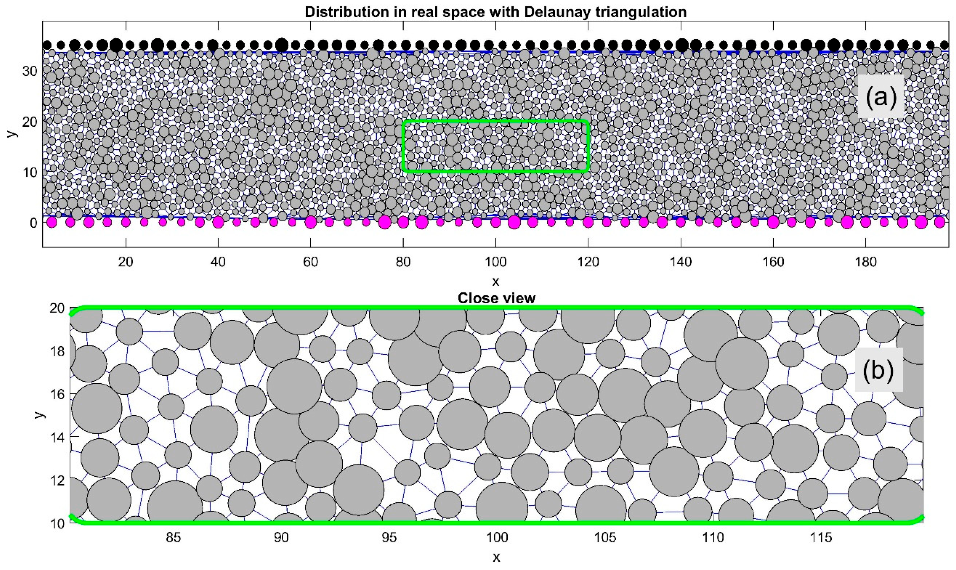
Figure 1 demonstrates an ensemble resulting from the interaction forces defined in Equations (5)–(7). It shows a typical instantaneous particle distribution between the upper and lower surfaces. These surfaces contain fixed particles (depicted in black and magenta), which move in opposite horizontal directions. The same interaction rules apply to these surface-bound particles as to the internal ones.
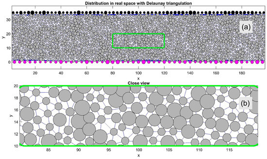
Figure 1.
(a) Instantaneous particle distribution between oppositely moving upper and lower surfaces with fixed surface particles (black and magenta). Internal particles are linked by Delaunay triangulation (thin lines) to identify nearest neighbors and analyze the lattice order. (b) A magnified view of the green-marked region.
The internal particles in Figure 1 are interconnected using Delaunay triangulation (thin lines), which allows for rapid identification of each particle’s nearest neighbors. This triangulation is essential for characterizing the system’s structural order and its temporal evolution. For better visualization, a magnified view of the central region (highlighted by a green rectangle in subplot (a)) is shown in subplot (b). The main system includes a diverse mix of particles with varying radii , and their dynamic behavior is further illustrated in Supplementary Movie Test_1.mp4. This video shows spontaneous ordering and motion of particles between two plates, including effects of mutual repulsion and aggregation, and how these behaviors relate to the boundaries.
Realistic boundary motion can be achieved based on the chosen simulation scenario and associated boundary conditions. For simplicity, particles may be confined within a rectangular domain with reflective vertical and horizontal boundaries. However, for more realistic modeling, surface particles are allowed to move vertically. To simulate quasi-infinite motion in the horizontal direction (which enhances statistical reliability), periodic boundary conditions (i.e., cylindrical geometry) were used. This approach was employed in all supplementary movies.
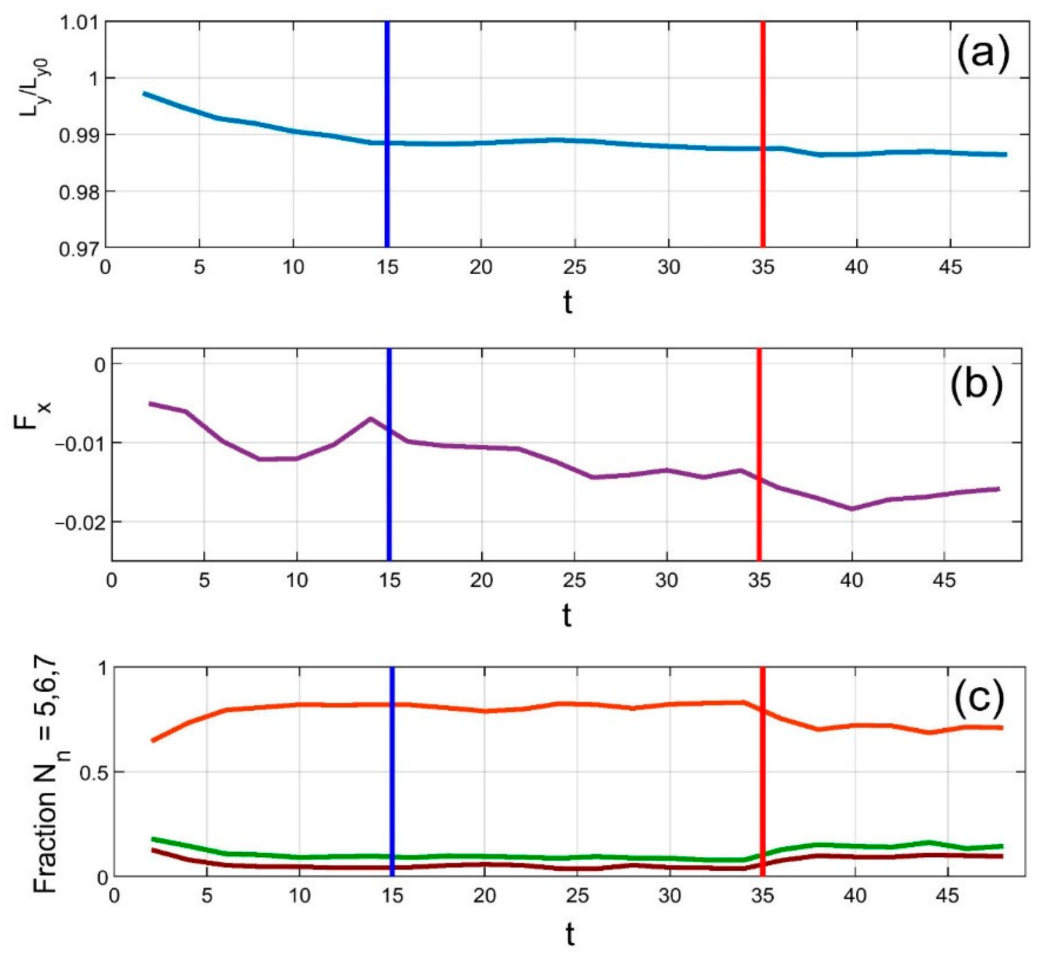
Figure 2 presents time-dependent correlations among several key system parameters: the vertical position of the upper plate, the horizontal force (interpreted as friction), and the fractions of particles with five, six, and seven neighbors. Vertical blue lines indicate the end of the initialization phase, during which the system self-organizes from a random initial configuration into an equilibrium state. During this period, the system spontaneously forms a hexagonal lattice, significantly increasing the proportion of particles with six neighbors despite variations in particle size.
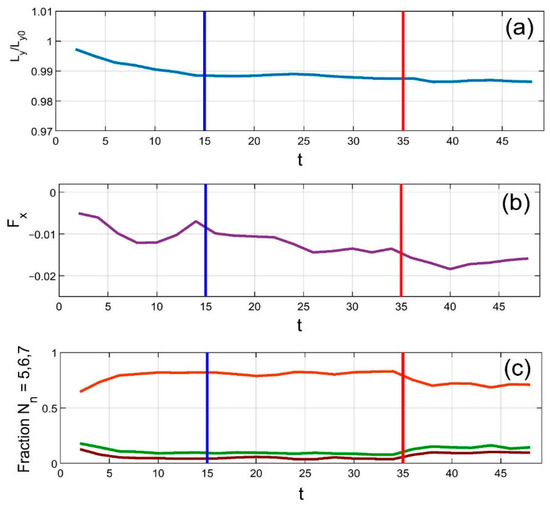
Figure 2.
Time evolution of key system parameters: (a) vertical upper plate position, (b) horizontal (friction) force, and (c) fractions of particles with 5, 6, and 7 neighbors (green, orange and dark red lines, respectively). The initial self-organization phase ends at the vertical blue line, after which a near-perfect hexagonal order emerges (6 neighbors dominate). Heating begins at the vertical red line, disrupting the structure and increasing defects.
This ordered structure is maintained even during horizontal plate motion, up until the point when external heating is applied. This moment is marked by the vertical red line. As expected, the applied heating rapidly disrupts particle positions, increasing defects in the previously ordered hexagonal structure. In other words, the balance shifts from particles with six neighbors toward those with five or seven. This trend is clearly visible in subplot (c), where the orange curve (six neighbors) declines, while the other two rise.
Note that the colors of the curves—orange, green, and dark red—match those used in the visualizations in subsequent figures. Please also note that the fraction of particles with 5, 6, or 7 neighbors does not sum to exactly 1, since particles with fewer or more neighbors are untracked in this figure. Near equilibrium, such anomalies are rare and have a minimal impact on the system’s collective behavior.
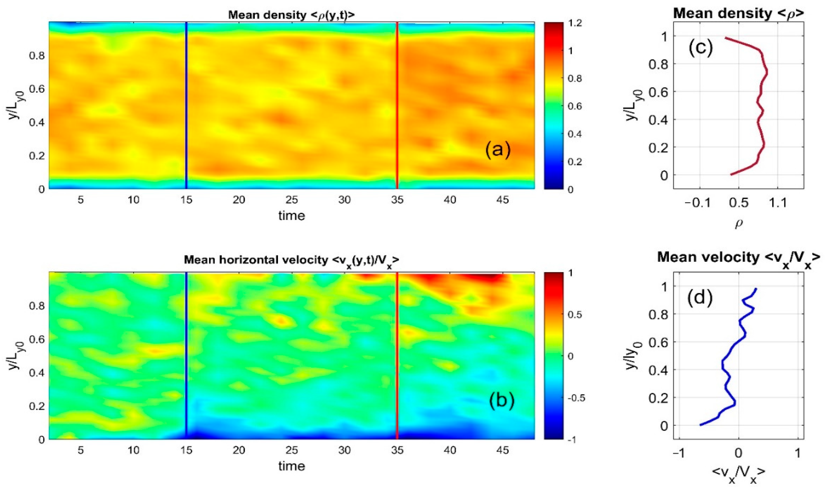
The dynamic evolution in Supplementary Movie Test_1.mp4 is captured in static form through time–space maps, shown in Figure 3a,b. Here, the discrete particle distributions are smoothed into continuous density fields and averaged along the horizontal axis. Instantaneous density and velocity distributions appear in subplots (c) and (d). These continuous values are also accumulated over time and displayed as color maps, with individual color bars in (a) and (b) reflecting different physical quantities.

Figure 3.
Dynamic evolution of the system from Supplementary Movie Test_1.mp4 is shown statically as time–space maps in subplots (a,b), where particle distributions are smoothed into a continuous density using Gaussian convolution and averaged horizontally. Vertical lines indicate the end of the initial phase and the start of heating, as in the previous figure. Instantaneous density and velocity are shown in subplots (c,d).
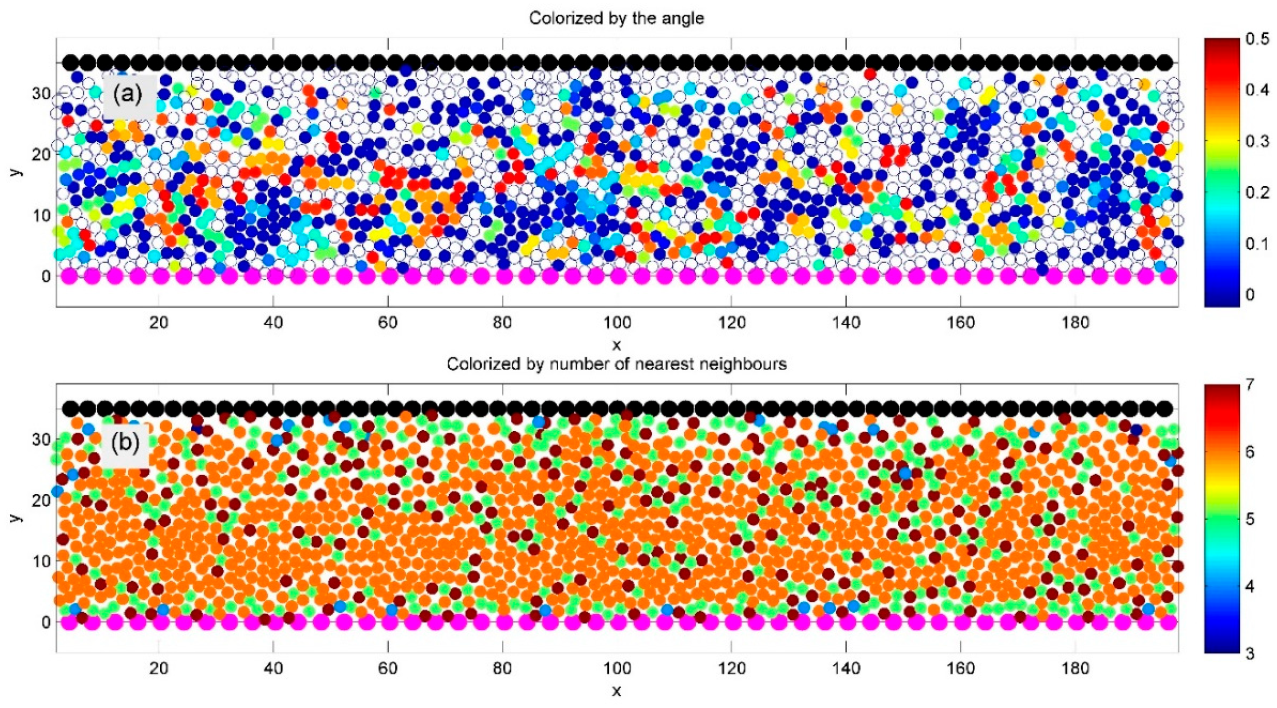
After testing a general model with particles of varying sizes, we focused next on a simplified, but more practically relevant, version with identical particles. Figure 4 shows such a system, where all particles have equal radii as well as identical adhesion belts and interaction parameters, simulated using the general model described in Figure 1 at a fixed average density.
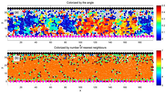
Figure 4.
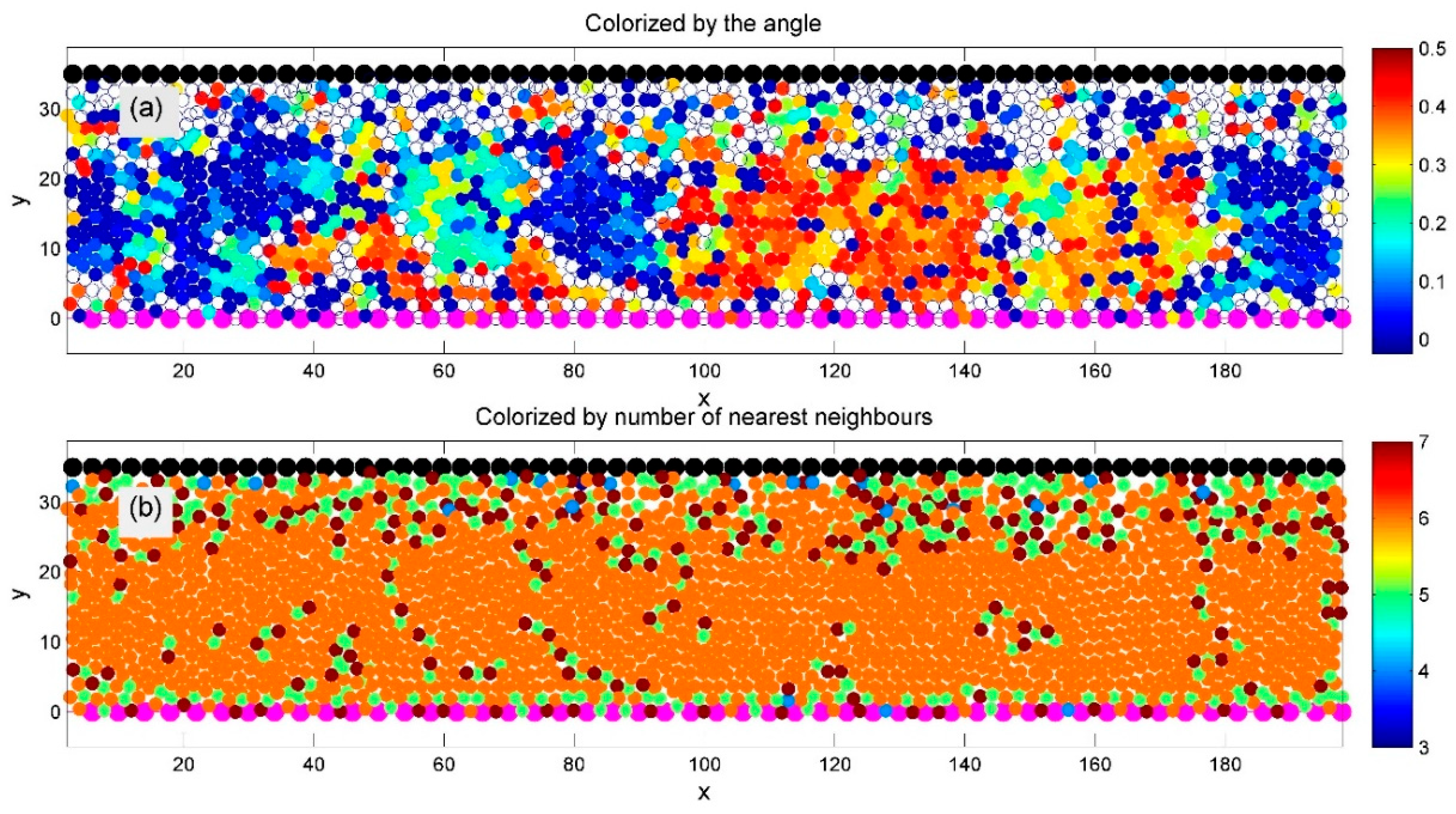
A regular-density model with identical particles (equal radii and interaction parameters) is simulated using the general setup from Figure 1. Surface particles are colored back and magenta. Subplot (a) shows domains with different lattice orientations, colorized by the sine of the orientation angle. After the initial transient phase, a well-ordered hexagonal structure emerges, indicated by orange-colored particles with six neighbors in subplot (b). Domain boundaries, marked by chains of 5- and 7-fold defects, appear in green and dark red.
A spontaneously formed regular hexagonal structure is clearly visible in both subplots (a) and (b). This order is confirmed in subplot (b) by the dominance of orange-colored particles, indicating six neighbors. The system also exhibits distinct domains of hexagonal order, each with a different crystal lattice orientation.
In subplot (a), domain orientation is color-coded by the sine of the angle between each particle and its nearest neighbor. Domain boundaries are visible in subplot (b) as chains of defects—particles with five or seven neighbors—marked in green and dark red, respectively.
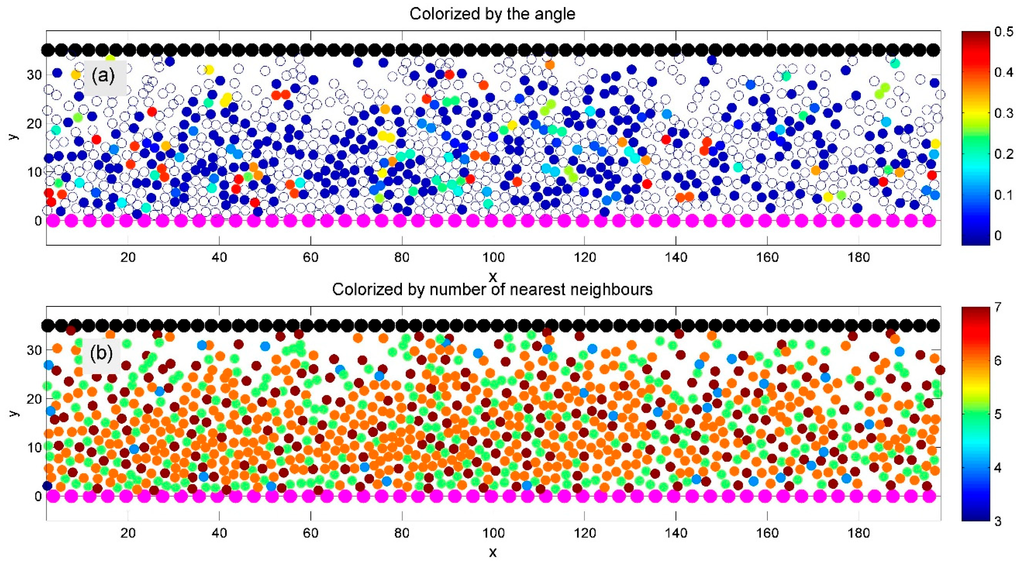
To complete the evaluation of the model, we also examined the system behavior at lower average densities. The results are presented in Figure 5 and Figure 6.
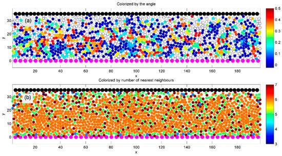
Figure 5.
Similar to Figure 4, but at lower average density. Surface particles are colored back and magenta. Subplot (a) shows domains colorized by the sine of the orientation angle, with visibly more disorder compared to the high-density case. Subplot (b) still shows well-defined ordered domains (orange), though many particles now appear light green and blue, indicating fewer neighbors. Some less distinct domains with preferred crystal lattice orientations are also visible.

Figure 6.
Same as Figure 4 but at much lower density. Surface particles are colored back and magenta. Subplot (a) shows domains colorized by the sine of the orientation angle, but coherent domains are barely identifiable. In subplot (b), large orange domains are absent, and many more light green and blue particles indicate increased defects and lower symmetry.
The systems shown in Figure 5 and Figure 6 show the same system at lower average densities. In Figure 5, ordered domains remain visible—particularly in subplot (b), where particles in these regions appear orange, indicating six neighbors. However, many particles are now light green and blue, reflecting a reduced number of neighbors in the Delaunay triangulation. Some domains with preferred lattice orientations are still distinguishable, though less clearly. In contrast, Figure 6 shows no large orange domains; most particles are light green and blue, indicating a high level of structural defects and reduced symmetry.
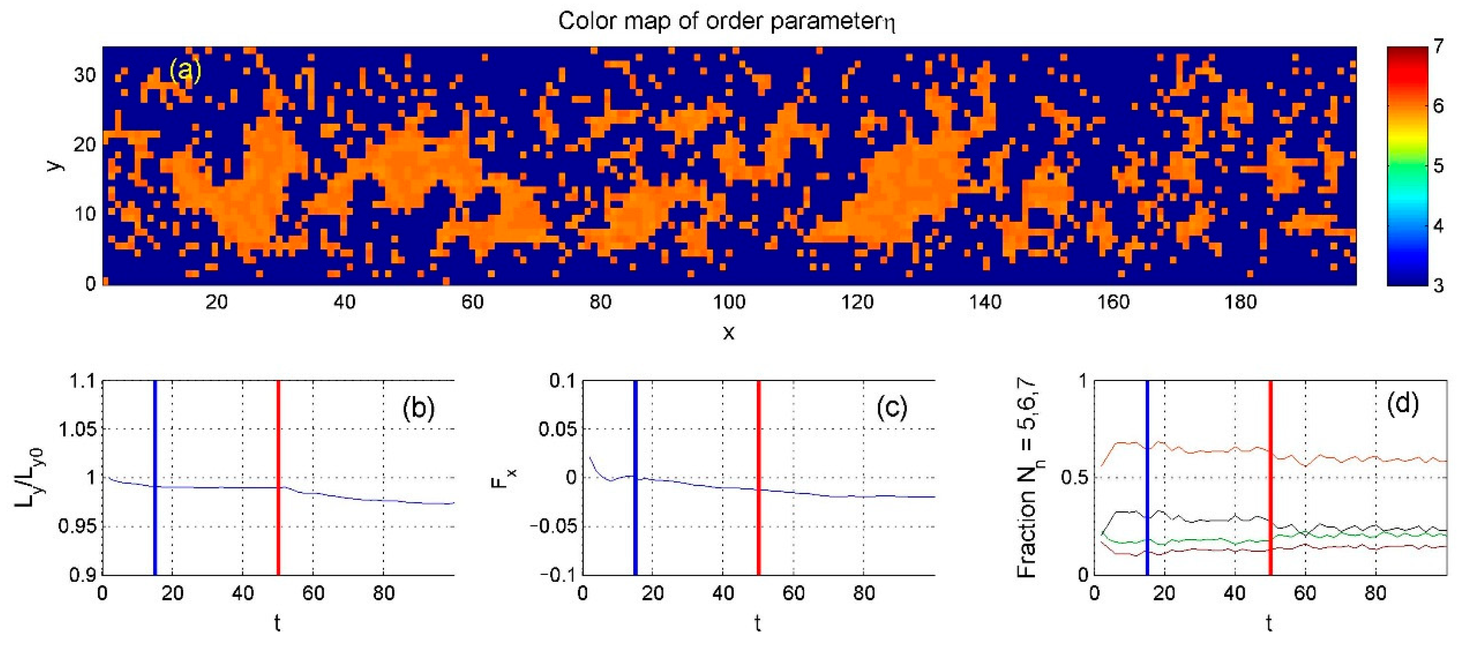
Scatter plots such as the above provide a good general picture of the system’s structure and dynamics, but a continuous approach is more effective for quantitative analysis. To this end, we computed a continuous “order parameter” using Gaussian convolution to estimate the local neighbor density, as shown in Figure 7, where orange regions once again indicate areas with ideal hexagonal order. The figure also shows the time-dependent position of the upper boundary, determined by the balance between the applied force and the internal particle pressure (Equation (8)). Subplot (c) shows the total friction force resulting from the relative motion of the upper and lower boundaries.
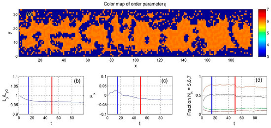
Figure 7.
(a) Continuous domain structure demonstrated by smoothed order parameter (high-density case). Note the large domains with ideal hexagonal order (orange). (b) Temporal evolution of the upper boundary position, (c) total friction force—negative due to stronger lower-surface coupling—and (d) neighbor fractions with an order parameter (black line) indicating structural order and fractions of particles with 5, 6, and 7 neighbors (green, orange and dark red lines, respectively). The blue and red vertical lines in (b–d) indicate the end of the initialization phase and the beginning of the heating phase, respectively.
Subplot (d) shows the time-dependent fractions of particles with different coordination numbers, represented by green, orange, and red curves—matching the color scheme used in the scatter plots. The black curve shows the “order parameter,” defined as the difference between the fraction of six-neighbor particles and the sum of the other two. After heating begins (marked by the red line), this balance shifts, and the system becomes more disordered.
The same calculations were repeated for different average densities, with results shown in Figure 8 and Figure 9. The most notable difference in Figure 9 is that the order parameter fluctuates around zero, indicating a nearly disordered system where the fraction of six-neighbor particles is roughly equal to the combined fraction of the others.

Figure 8.
(a) Continuous domain structure demonstrated by smoothed order parameter with lower average density . Note the smaller ordered (orange) domains. (b) Temporal evolution of the upper boundary position, (c) total friction force, (d) neighbor fractions with an order parameter (black) indicating structural order. Note the much lower order parameter compared to Figure 7. The blue and red vertical lines in (b–d) indicate the end of the initialization phase and the beginning of the heating phase, respectively.
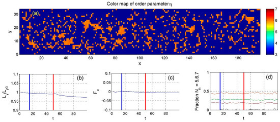
Figure 9.
(a) Continuous domain structure demonstrated by smoothed order parameter with the lowest overall density (b) Temporal evolution of the upper boundary position, (c) total friction force, (d) neighbor fractions with an order parameter (black) indicating structural order. Unlike Figure 7 and Figure 8, the order parameter and the force of friction fluctuate around zero. The blue and red vertical lines in (b–d) indicate the end of the initialization phase and the beginning of the heating phase, respectively.
We further considered the simultaneous time evolution of the spatially distributed density , kinetic energy , horizontal velocity , and their values integrated along the -coordinate:
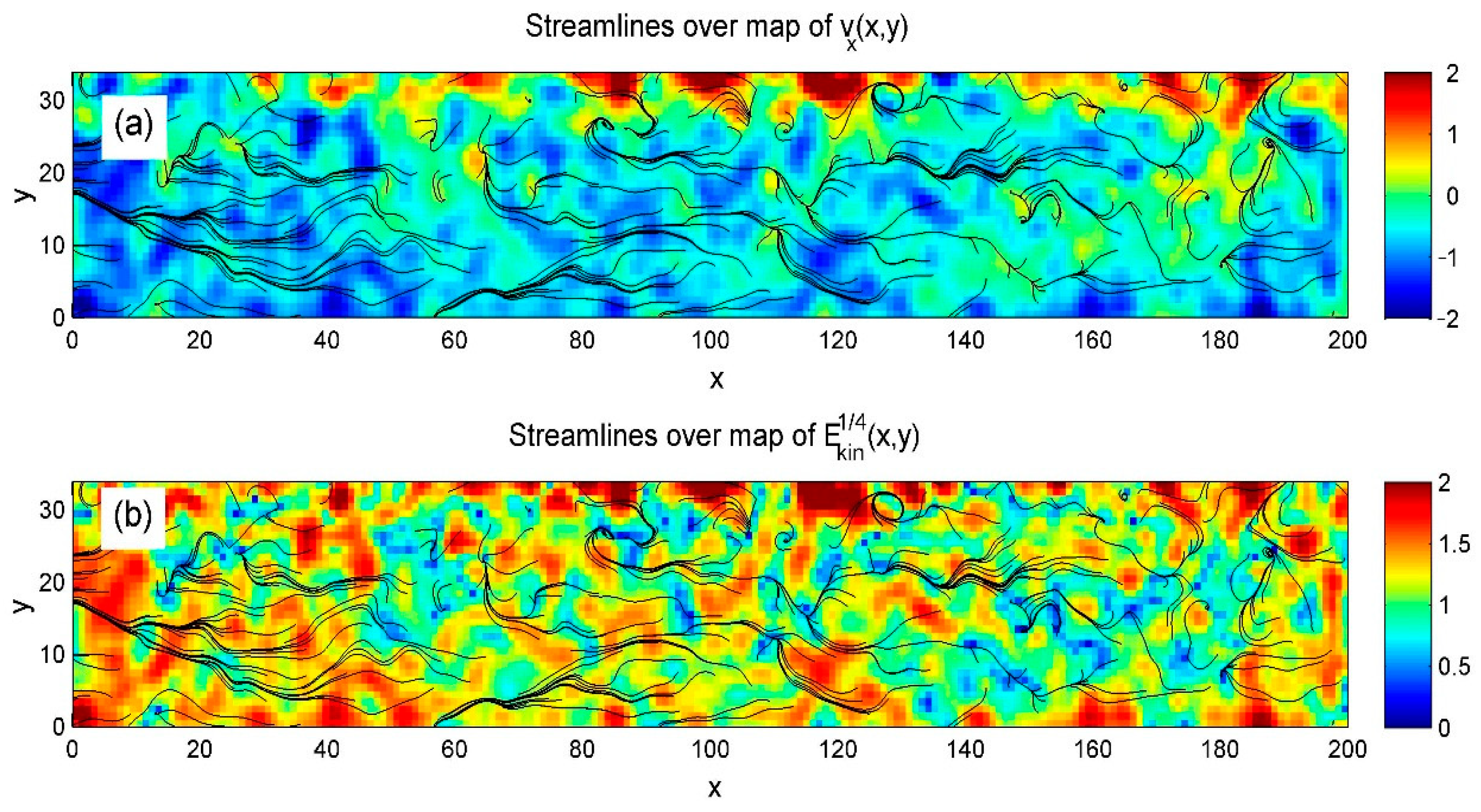
Although horizontal velocity is central to this study, both velocity components contribute to the formation of streamlines. Therefore, we calculated streamline maps at each time step, with and without heating. The streamlines are shown in Figure 10. Their dynamic evolution—highlighting flow complexity and turbulence, especially under heating—is illustrated in Supplementary Movie Stream.mp4.
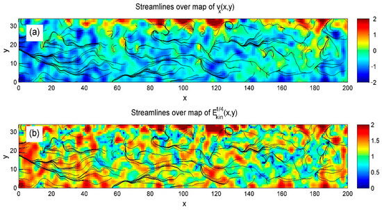
Figure 10.
Streamlines from Gaussian-convolved data are shown over horizontal velocity (a) and kinetic energy (b) to highlight laminar flow in the bulk and turbulence near the heated upper surface. This contrast is especially clear in Supplementary Movie Stream.mp4.
The detailed flow complexity is not captured in the integrated time-dependent maps below. However, these integrations effectively reveal how key global values evolve over time as shear and heating are applied sequentially. As with the order parameter, we present the results as horizontally averaged time–space diagrams. The summaries for three average densities are shown in Figure 11, Figure 12 and Figure 13 and the corresponding movies Regular_1.mp4, Regular_2.mp4, and Regular_3.mp4.
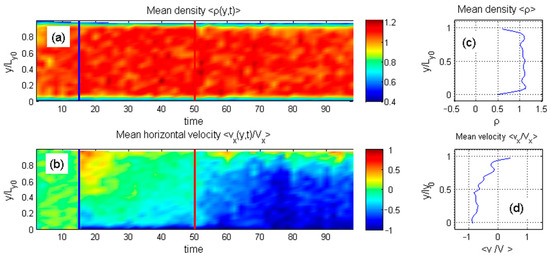
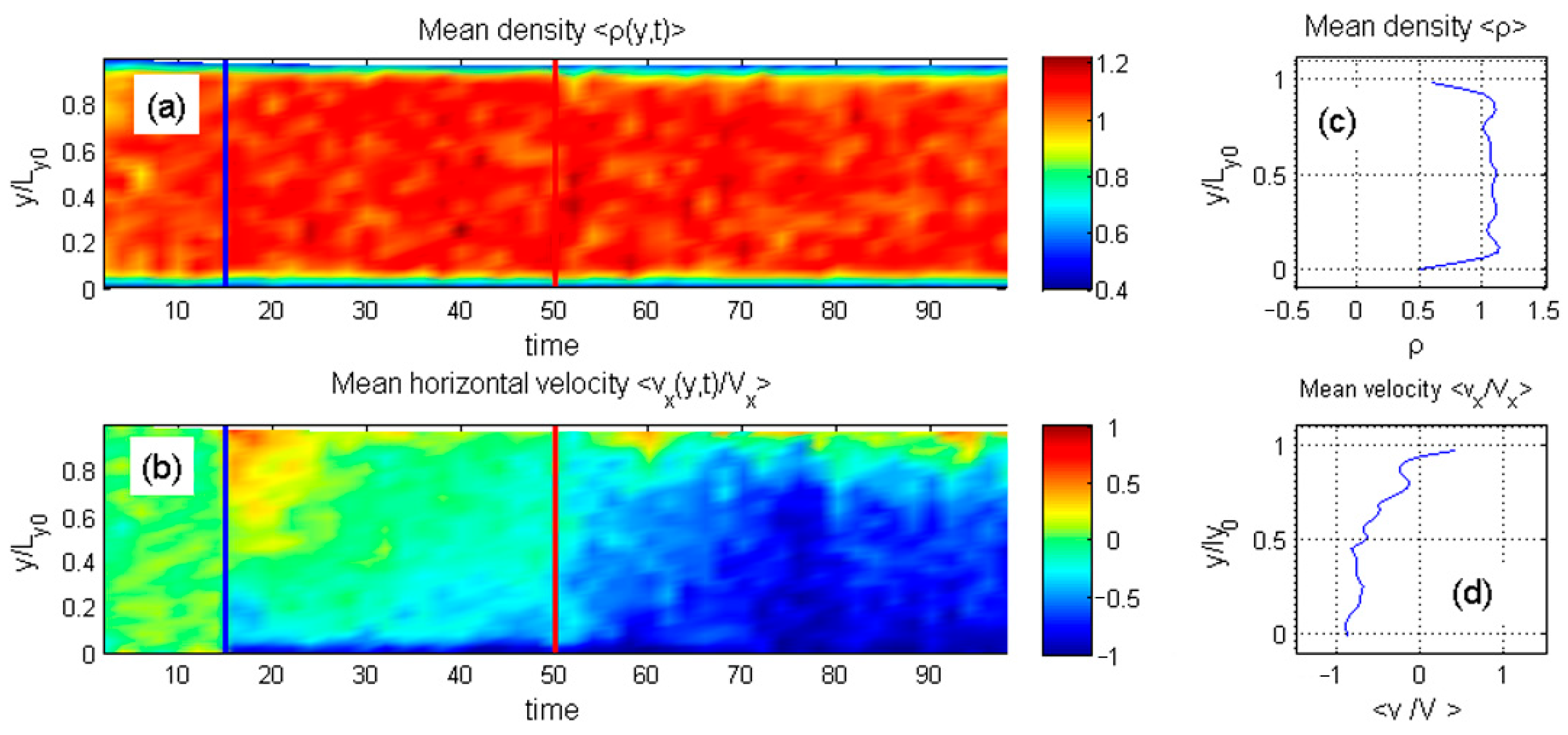
Figure 11.
Space-time maps subplots of (a) the mean density and (b) mean horizontal velocity for a high-density configuration. The vertical blue and red lines indicate the end of initialization and the beginning of heating, respectively. The final profiles of density and velocity are shown in (c,d). These space-time maps highlight a key result of the study: in a sufficiently dense system, heating from the upper surface causes the internal particles to follow the motion of the bottom surface, whose fixed particle spacing closely matches the typical distance between the mobile particles.

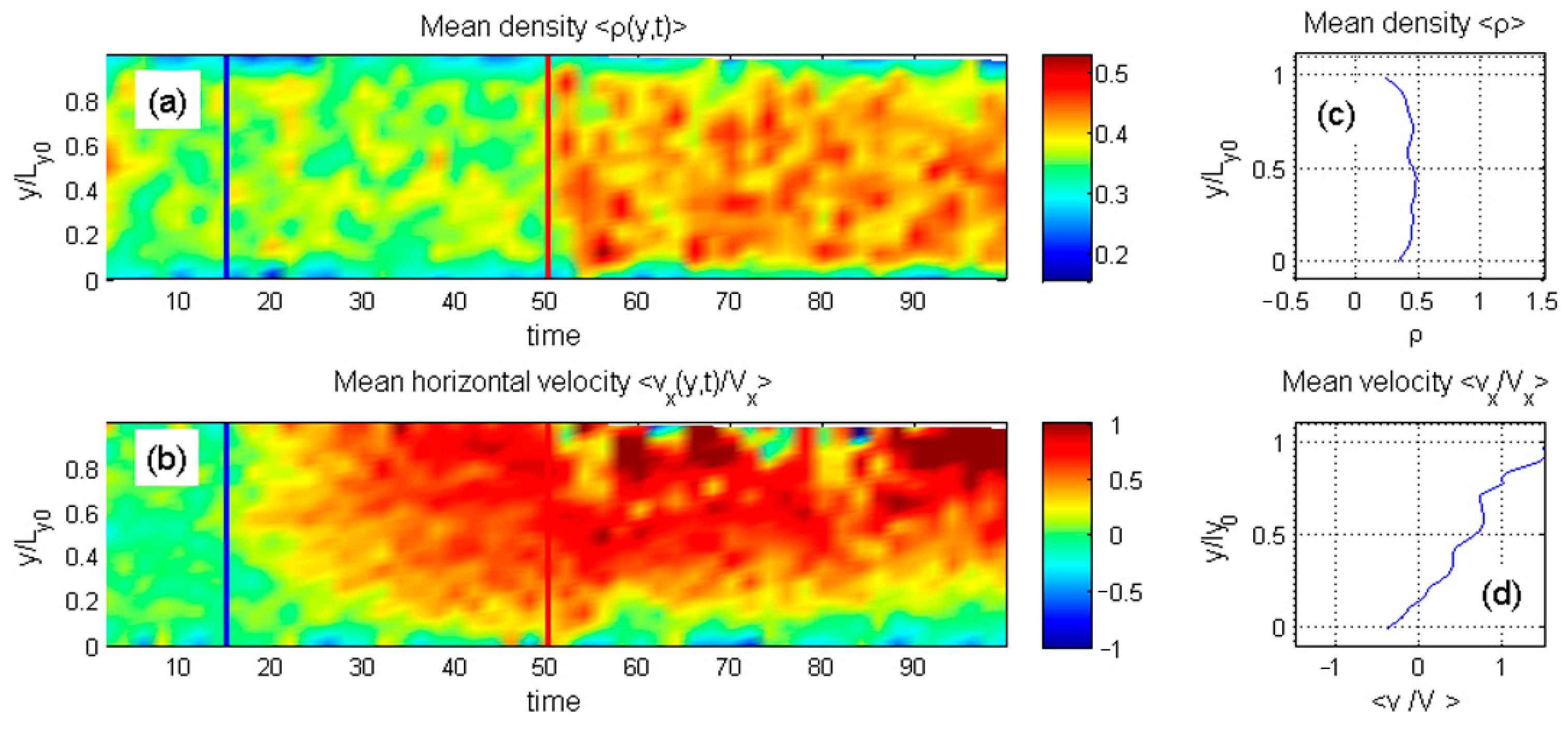
Figure 12.
Space-time maps subplots of (a) the mean density and (b) mean horizontal velocity for a lower-density configuration. The vertical blue and red lines indicate the end of initialization and the beginning of heating, respectively. The final profiles of density and velocity are shown in (c,d). The particles gradually redistributed in space to reduce interlocking with the commensurate lower substrate causing linear distribution of the velocity along the vertical coordinate.

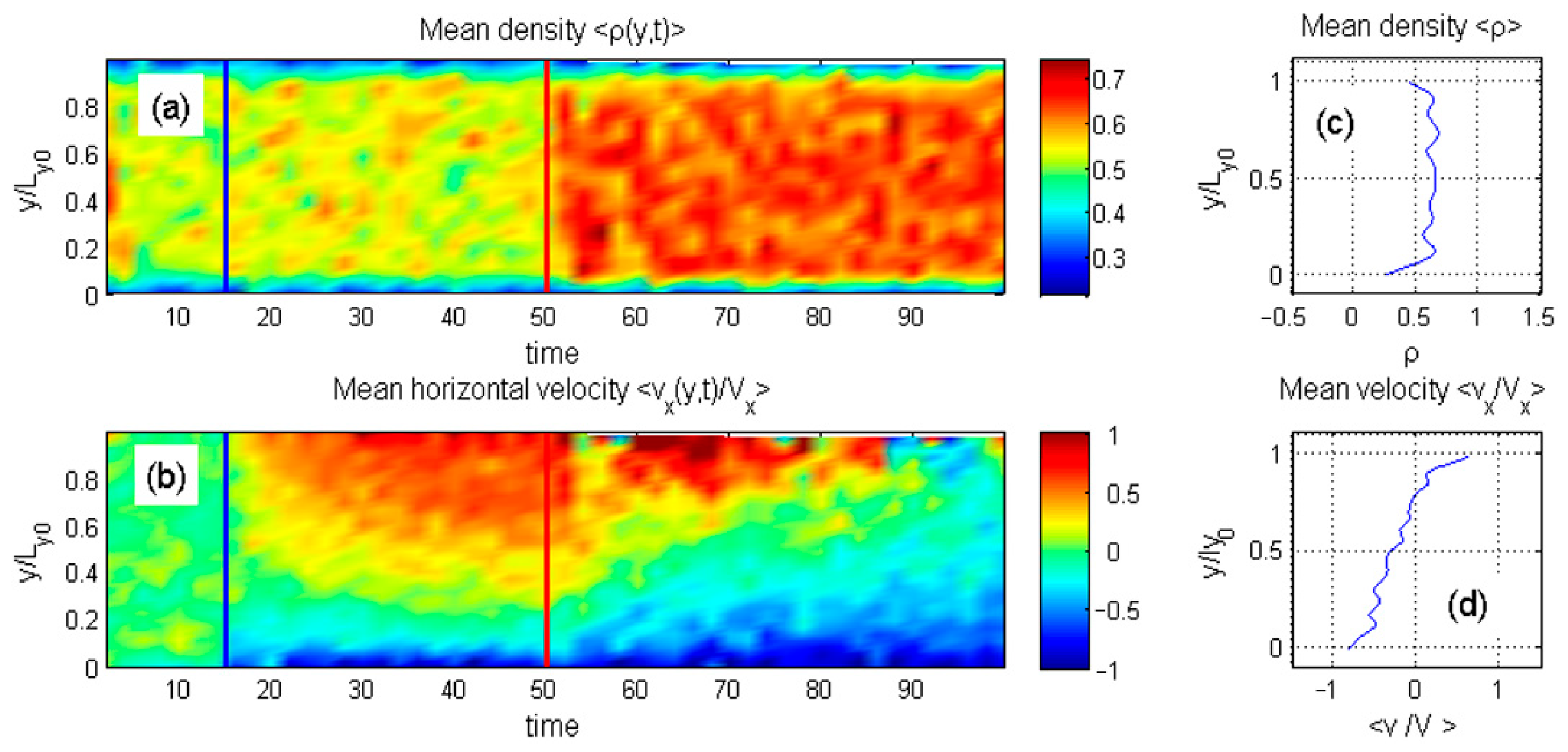
Figure 13.
Space-time maps subplots of (a) the mean density and (b) mean horizontal velocity for the lowest-density configuration. The vertical blue and red lines indicate the end of initialization and the beginning of heating, respectively. The final profiles of density and velocity are shown in (c,d). Particles shift toward the center, reducing interlocking with both surfaces. However, thermal fluctuations near the heated upper surface occasionally enhance coupling, shifting overall motion to the right—opposite to the leftward flow in Figure 11.
These maps highlight the study’s main findings. Initially, in the absence of heating, the dense system transitions into a near-laminar flow. The lower region, where surface particle spacing matches internal particle spacing, moves faster in the negative direction than the upper region, creating a vertical velocity gradient that becomes nearly linear (see Regular_1.mp4).
When heating is applied, this velocity contrast increases. In the steady state, most of the system moves with the lower surface, while only the uppermost layers retain positive velocity. This shift appears as a step-like velocity profile in subplot (d) of Figure 11. Although heating slightly affects the density distribution, this influence is minimal in the high-density case.
The intermediate-density system shows the richest behavior. As seen in Regular_2.mp4 and Figure 12, the particle density redistributes during the process. Initially, without heating, internal particles move in the positive direction. Once heating is applied, the vertical density profile changes, altering the contact with the upper surface. After a transient phase, the internal particles reverse direction and begin moving in the negative direction.
Finally, the time-dependent behavior of the low-density system is shown in Regular_3.mp4 and Figure 13. Here, the particle density concentrates near the center, reducing interlocking with both surfaces. Strong thermal fluctuations near the heated upper surface occasionally enhance or weaken coupling with the surface particles, shifting the velocity balance in favor of rightward motion. This behavior contrasts sharply with the leftward flow seen in Figure 11.
5. Conclusions
A particle-based numerical model for the study of friction between two atomically flat surfaces separated by a fluid was developed and characterized. It was shown that the model leads to realistic behavior at different parameters of interaction and loading modes, such as temperature, density, external pressure, and mutual relative velocity of the surface plates. The system can assume solid, liquid, and gaseous states, depending on the effective temperature (kinetic energy caused by surface motion and random noise generated by spatially distributed Langevin sources).
The main part of the study was devoted to testing the model with a fluid system composed of equally sized particles in contact with two commensurate surfaces. It was established that the behavior of the system is mainly determined by the relative radius of the “fluid” and “surface” automata and by the parameters of adhesive interaction between them. It was shown also that heating of the system in different regions close to one of the plates can change the density of the “liquid” in its proximity, provoke a chaotization of the liquid dynamics, and result in dramatic transformation of the global structure and dynamics. Local heating can even essentially change the direction of the average flow. Such an intensive restructuring of the process may have practical applicability for a significant reduction in friction in general.
Supplementary Materials
The following supporting information can be downloaded at: https://www.mdpi.com/article/10.3390/computation13070155/s1. Supplementary Movie Test_1.mp4: This video demonstrates the dynamic evolution of particle configurations between two surfaces moving in opposite horizontal directions. The plates are coated with fixed surface particles that are color-coded in black and blue, respectively. Supplementary Movie Stream.mp4: Dynamically changing (plotted with a discrete time-steps) continuous medium obtained by the Gaussian convolution of the movable discrete automata. The streamlines are plotted over the spatial densities of the horizontal velocity and kinetic energy to illustrate the contrast between the laminar flow inside the system and turbulence in the vicinity of heated upper substrate. Supplementary Movie Regular_1.mp4: Motion of the high-density system (with equal radii for all particles) recorded dynamically. The scatter plot is colorized by number of nearest neighbors as shown by the color bar. Integral values of the distance between the plates and friction force, as well as fractions of the subsystems with and, are plotted below the scatter. Time–space diagrams accumulating simultaneously with the dynamic process are depicted in the right panel of the movie. Integral density averaged over x and distribution of horizontal velocity depending on vertical coordinate y are plotted in the right subplots of this panel, respectively. Supplementary Movie Regular_2.mp4: The same as in the Supplementary Movie Regular_1.mp4 calculated at intermediate density . Of particular note are the changes in velocity distribution in the far-right subplot of the movie during the process, especially with heating enabled. Supplementary Movie Regular_3.mp4: The same as in the Supplementary Movie Regular_1.mp4 calculated at small density . One can notice dramatic chaotization of the motion produced by heating (in comparison to the original movie Regular_1.mp4) accompanied by transformations of the velocity distribution shown in the far-right subplot.
Author Contributions
Conceptualization, V.L.P. and M.P.; methodology, V.L.P., M.P. and A.E.F.; software, A.E.F.; investigation, A.E.F.; writing—original draft preparation, A.E.F., M.P. and V.L.P.; writing—review and editing, M.P. and V.L.P.; supervision, V.L.P.; funding acquisition, V.L.P. All authors have read and agreed to the published version of the manuscript.
Funding
This research was funded by the Deutsche Forschungsgemeinschaft (DFG), project number 554322826 and by the Samarkand State University.
Data Availability Statement
The original contributions presented in this study are included in the article/Supplementary Materials. Further inquiries can be directed to the corresponding authors.
Conflicts of Interest
The authors declare no conflicts of interest.
References
- Thompson, P.A.; Robbins, M.O. Shear flow near solids: Epitaxial order and flow boundary conditions. Phys. Rev. A 1990, 41, 6830–6837. [Google Scholar] [CrossRef] [PubMed]
- Lauga, E.; Brenner, M.P.; Stone, H.A. Microfluidics: The no-slip boundary condition. In Springer Handbook of Experimental Fluid Mechanics; Springer: Berlin/Heidelberg, Germany, 2007; pp. 1219–1240. [Google Scholar] [CrossRef]
- Popov, V.L. Contacts with negative work of “adhesion” and superlubricity. Front. Mech. Eng. 2020, 5, 73. [Google Scholar] [CrossRef]
- Hod, O.; Meyer, E.; Zheng, Q.; Urbakh, M. Structural superlubricity and ultralow friction across the length scales. Nature 2018, 563, 485–492. [Google Scholar] [CrossRef] [PubMed]
- Socoliuc, A.; Bennewitz, R.; Gnecco, E.; Meyer, E. Transition from stick-slip to continuous sliding in atomic friction: Entering a new regime of ultralow friction. Phys. Rev. Lett. 2004, 92, 134301. [Google Scholar] [CrossRef] [PubMed]
- Han, T.; Zhang, S.; Zhang, C. Unlocking the secrets behind liquid superlubricity: A state-of-the-art review on phenomena and mechanisms. Friction 2022, 10, 1137–1165. [Google Scholar] [CrossRef]
- Dzyaloshinskii, I.E.; Lifshitz, E.M.; Pitaevskii, L.P. The general theory of van der Waals forces. Adv. Phys. 1961, 10, 165–209. [Google Scholar] [CrossRef]
- Meurk, A.; Luckham, P.F.; Bergström, L. Direct measurement of repulsive and attractive van der Waals forces between inorganic materials. Langmuir 1997, 13, 3896–3899. [Google Scholar] [CrossRef]
- Ye, Y.; Li, Y.; Lin, Q.; Zeng, S.; Zhou, X.; Zhang, C. Casimir repulsive-attractive transition between liquid-separated dielectric metamaterial and metal. Phys. Rev. B 2018, 98, 035410. [Google Scholar] [CrossRef]
- Zhou, Y.; Wang, A.; Müser, M.H. How thermal fluctuations affect hard-wall repulsion and thereby Hertzian contact mechanics. Front. Mech. Eng. 2019, 5, 67. [Google Scholar] [CrossRef]
- Pinon, A.V.; Klinke, C.; Berg, S.; Yamakov, V. Thermal effects on van der Waals adhesive forces. Phys. Rev. B 2016, 93, 035424. [Google Scholar] [CrossRef]
- Levitas, V.I.; Idesman, A.V.; Palakala, A.K. Phase-field modeling of fracture in liquid. J. Appl. Phys. 2011, 110, 033531. [Google Scholar] [CrossRef]
- Denisov, S.; Filippov, A.; Klafter, J.; Urbakh, M. From deterministic dynamics to kinetic phenomena. Phys. Rev. E 2004, 69, 042101. [Google Scholar] [CrossRef] [PubMed]
- Shilko, E.V.; Dmitriev, A.I.; Balokhonov, R.R.; Romanova, V.A. Multiscale Modeling and Computer-Aided Design of Advanced Materials with Hierarchical Structure. Phys. Mesomech. 2024, 27, 493–517. [Google Scholar] [CrossRef]
- Vanossi, A.; Bechinger, C.; Urbakh, M. Structural lubricity in soft and hard matter systems. Nat. Commun. 2020, 11, 4657. [Google Scholar] [CrossRef]
- Monaghan, J.J. An introduction to SPH. Comput. Phys. Commun. 1988, 48, 88–96. [Google Scholar] [CrossRef]
- Radjai, F.; Dubois, F. Discrete-Element Modeling of Granular Materials; Wiley-ISTE: London, UK, 2011. [Google Scholar]
- Pöschel, T.; Schwager, T. Computational Granular Dynamics: Models and Algorithms; Springer: Berlin, Germany, 2005. [Google Scholar] [CrossRef]
- Dmitriev, A.I.; Nikonov, A.Y.; Filippov, A.E.; Psakhie, S.G. Molecular dynamics study of the evolution of rotational atomic displacements in a crystal subjected to shear deformation. Phys. Mesomech. 2019, 22, 375–381. [Google Scholar] [CrossRef]
- Österle, W.; Dmitriev, A.I.; Kloß, H. Possible impacts of third body nanostructure on friction performance during dry sliding determined by computer simulation based on the method of movable automata. Tribol. Int. 2012, 48, 128–135. [Google Scholar] [CrossRef]
- Rudge, R.E.D.; van de Sande, J.P.M.; Dijksman, J.A.; Scholten, E. Uncovering friction dynamics using hydrogel particles as soft ball bearings. Soft Matter 2020, 16, 3821–3828. [Google Scholar] [CrossRef]
- Alazemi, A. Experimental study of the lubrication mechanism of micro-spherical solid particles between flat surfaces. Lubricants 2021, 9, 81. [Google Scholar] [CrossRef]
- Paul, W.B. Molecular dynamics simulation, elementary methods. Adv. Mater. 1993, 5, 223–225. [Google Scholar] [CrossRef]
- Fermi, E.; Pasta, J.; Ulam, S. Studies of Nonlinear Problems, Los Alamos Report No. LA-1940; Fermi, Ed.; Collected Papers: Chicago, IL, USA, 1955; Volume 2, pp. 978–988. [Google Scholar]
- Langevin, P. On the theory of Brownian motion. C. R. Acad. Sci. Paris 1908, 146, 530–533. [Google Scholar]
- Landau, L.D.; Lifshitz, E.M. Mechanics: Course of Theoretical Physics; Pergamon Press: Oxford, UK, 1976; Volume 1. [Google Scholar]
- Filippov, A.E.; Popov, V.L. Numerical simulation of dynamics of block media by movable lattice and movable automata methods. Facta Univ. Ser. Mech. Eng. 2023, 21, 553–562. [Google Scholar] [CrossRef]


Disclaimer/Publisher’s Note: The statements, opinions and data contained in all publications are solely those of the individual author(s) and contributor(s) and not of MDPI and/or the editor(s). MDPI and/or the editor(s) disclaim responsibility for any injury to people or property resulting from any ideas, methods, instructions or products referred to in the content. |
© 2025 by the authors. Licensee MDPI, Basel, Switzerland. This article is an open access article distributed under the terms and conditions of the Creative Commons Attribution (CC BY) license (https://creativecommons.org/licenses/by/4.0/).