Abstract
This paper deals with queueing models, in which the number of customers is described by a (inhomogeneous, in general) birth–death process. Depending on the choice of the type of intensities for the arrival and service of customers, the system can either have impatience (in which, as the queue length increases, the intensities of arrival decrease and the intensities of service increases) or attraction (in which, on the contrary, as the queue length increases, the intensities of the arrival of customers increase and service intensities decrease). In this article, various types of such models are considered, and their transient and limiting characteristics are computed. Furthermore, the rate of convergence and related bounds are also dealt with. Several numerical examples illustrate the proposed procedures.
1. Introduction
This paper aims to show that, using (inhomogeneous) birth–death processes (BDPs) with state-dependent intensities, one can describe and investigate simple queuing theory models with different types of customer and server behavior.
In both the case of ergodicity and the case of null ergodicity, it is possible to obtain explicit estimates of the rate of convergence. In the ergodic case, these estimates also allow us to study the boundaries of perturbation and approximations using truncations and to compute the main limiting characteristics of the corresponding model. Thus, by selecting the model parameters, it is possible to control the queueing system.
We consider a general queueing system of type , in which the intensities of the arrival and service of customers characterize the corresponding behavior (of customers and servers) in the queue.
The earliest models relate to queues where potential customers are discouraged by queue length; see [1,2,3,4]. This is reflected in the corresponding choice of monotonically decreasing intensities for the arrival of customers. Models with impatient customers began to be actively studied, in which the property of impatience was most often described by an increase in service intensities; see, for example, [5,6,7,8,9,10,11].
Further, queues with encouragement or with a server that works less effectively as the queue length increases are described by processes with increasing intensity of customer arrivals as the queue grows, or decreasing intensity of service; see [12,13]. As a result, the influence of the nature of the queue on the corresponding BDP can be taken into account due to the corresponding behavior of the intensities of the arrival/service of requests.
As one can see, most studies by other authors are devoted to constructing a particular solution at the initial stage of the system’s existence, usually for stationary systems. Often, they simply obtain a solution using purely numerical methods—uniformity, modeling, and Runge–Kutta methods—which, in general, do not provide useful information about the system; therefore, unlike the listed studies, the goal of this article is to construct a LIMIT solution, i.e., a stable solution that is practically independent of the initial state. Without knowing the convergence rate, it is not known when the limit solution has been reached. Comparison at the end of the period or (at constant intensities) of some interval is not enough to know whether the limit solution has been reached. In particular (for - periodicity), to achieve the limit regime, it is necessary to cut the system into the interval until is not less than the required accuracy. Here, is the convergence rate parameter. Another approach is to calculate the value of at which the limit solution is found. A table with a series of examples comparing these approaches is presented below. Note that, as the graphs below show, the actual value of is usually less than the expected value. It is worth noting that a comparison of numerical methods can be found in studies from the 1970s. Regarding relatively modern ones, we can use [14]. The Runge–Kutta method is distinguished by its guaranteed accuracy and is therefore often chosen as a reference in numerical experiments. In particular, in this work, we completed our calculations using it.
The main role in this work is played by the examples of different types of BDPs considered, describing the corresponding models; for each type of system, the derivation of the estimates of the rate of convergence and the construction of the main limiting characteristics are shown. Perturbation bounds and approximation errors using truncations can then be formally obtained by the methods described in [15].
2. Model Description and Main Results
Let be a queueing system with arrival and service rates and , respectively, and let be the corresponding queue-length process. Then, is a BDP with infinite state space , intensity matrix Q, and transposed intensity matrix . Then, matrix has the following form:
We will assume that the arrival and service intensities satisfy the following conditions: , , , and .
Denote the -norm by , with and for matrix .
We consider the corresponding forward Kolmogorov system:
as a differential equation in the space of sequences with bounded operator function A. Here, is the vector of state probabilities for BDP .
Moreover, if the queue is nonstationary, then the corresponding BDP is inhomogeneous and and are locally integrable on nonnegative functions such that for almost all . In this situation, the operator function is also bounded and locally integrable on .
Recall that
- A Markov chain is called null ergodic if as for any n and any initial condition ;
- A Markov chain is called ergodic if it has a stationary distribution such that as for any initial condition ;
- An inhomogeneous Markov chain is called weakly ergodic if as for any initial conditions and .
Also recall that the logarithmic norm of the operator function on gives us bounds for the rate of convergence for solutions of the corresponding linear differential equation and can be written as ; see all details in [15].
Consider an auxiliary “weight” sequence such that and the corresponding upper triangular matrix D:
We write for a vector .
Set
and
Theorem 1.
Let be a homogeneous BDP with positive intensities and . Let there exist limits and . Let . Then, the BDP is ergodic and there exists a sequence of positive numbers such that , , and .
Proof.
First, from our general scheme, we will carry out the following actions. From equality , we obtain . Hence, we have from (2) the following equation:
where , and
For bounding the rate of convergence, we consider the respective ’homogeneous’ equation in the corresponding space .
Then,
Now, we try to find a sequence such that all are the same and positive. The following reasoning is close to that carried out in [16]. Let . We denote . Hence, we set
and from (4), we recursively obtain the inequality
where .
Note that the derivatives of the functions are strictly greater than zero, and therefore the functions increase and have exactly one root. The function , has the unique root . Through recursion, we obtain from (8) that the function has a unique positive root, for example, and .
We have and
Let . From the definition of and the monotonicity of the functions , we have for all Hence, in the case considered, the set of solutions of is given by
□
Theorem 1 states that the sequence always exists and specifies the interval on which the number x is located, using which one can construct and obtain an exact estimate. Unfortunately, in the case of a countable number of states, knowledge of the interval does not allow one to find this x, and instead, a sequence giving a rough estimate is constructed in other ways. In the case of a finite number of states, this x can be found, and accordingly, the sequence will be obtained. Moreover, it will coincide with an eigenvector for the matrix B.
Consider now a null ergodic situation. Let there exist limits and such that . Set , . Consider now the diagonal matrix and the matrix :
Denote the sum of all elements of the k-th coloumn of by . One can see that implies that . Moreover, if is sufficiently small, then there exists such that , and so on. On the other hand, if we set , then we have . Hence, for the corresponding , all are positive for large k. Finally, we have , and all .
Then, for the corresponding weighted norm, we have, using the logarithmic norm, the following bound:
Hence,
for any n, where
This implies the following statement.
Theorem 2.
Let X be a homogeneous BDP with intensities and . Then, there exist limits and such that . Then, the BDP is null ergodic, and there exists a sequence of positive numbers such that bound (11) holds.
Remark 1.
All our considerations can be generalized to the case of arbitrary intensity functions and . Let us consider in particular the most important case of one-periodic intensities. We introduce the notation and . Then, the corresponding results for weakly ergodic and null ergodic situations follow from the existence of and for or , respectively, as shown below when considering specific models.
3. Numerical Examples
Since in real systems service requests usually arrive with variable intensities, the intensities below are taken to be periodic functions. Consider the queue-length process for four specific weakly ergodic models. We suppose that all intensity functions are periodic and that the ’basic’ intensities are and .
The intensities for the models are given below:
1. Model 1: the client gets scared when he sees the queue and does not join the queue—the rate of arrival decreases.
2. Model 2: the client thinks that something important is being sold when he sees the queue and joins the queue—the rate of arrival increases (a queue for Apple phones).
3. Model 3: with a large number of requests, network performance can drop (Ethernet)—the rate of service decreases.
4. Model 4: the client gets tired of waiting in the queue and leaves it (service intensity + escape) and the server switches to a more productive operating mode with a large number of requests, etc.—the rate of service increases.
The convergence pattern implies that over time the initial state in which the system was ceases to be important and has almost no effect on the behavior of the system. Thus, knowing the rate of convergence, one can find the value of after which all solutions of the system are almost indistinguishable from each other. Therefore, one can construct a limit solution from this using numerical methods.
For the four models, the results obtained can be combined in a table. In the examples, . Taking this into account, the norm of the difference in solutions was obtained.
Since in the examples and were taken, .
| Model 1 | Model 2 | Model 3 | Model 4 | |
| intensities | , | , | , | , |
| for ’basic’ intensities | ||||
| 180 | 300 | 380 | 300 | |
| error on interval | 0.0003 | 0.0008 | 0.0005 | 0.0008 |
To plot graphs and for ODE systems, we use standard libraries: Matplotlib and NumPy. We chose numpy because this library allows us to optimize calculations and achieve a higher execution speed for several reasons:
- NumPy is written primarily in the C programming language, which means that most operations are performed at the machine code level, which provides high performance compared to pure Python code;
- NumPy arrays are stored compactly and sequentially in RAM, which minimizes overhead and improves processor caching. When data are located close to each other, access to them becomes much faster, especially when processing large amounts of data;
- Operators and functions inside NumPy are pre-compiled and optimized for various platforms and processor architectures. This avoids the cost of interpreting Python code during program execution.
Here is an example of a code listing that allows a system of differential equations to be solved:
- import numpy as np
- from scipy.integrate import solve_ivp
- def function(t, y):
- return fA(t).dot(y)
- def main_calc_rk(init_vector, t_list, function):
- return solve_ivp(function, t_list, np.ravel(init_vector),
- method=’RK45’, atol=1e−12, rtol=1e−12)
- t_period = [0, t_end + 1]
- init_vector = np.zeros((n, 1))
- init_vector[0] = 1
- solution1 = main_calc_rk(init_vector, t_period, function)
- init_vector = np.zeros((n, 1))
- init_vector[−1] = 1
- solution2 = main_calc_rk(init_vector, t_period, function)
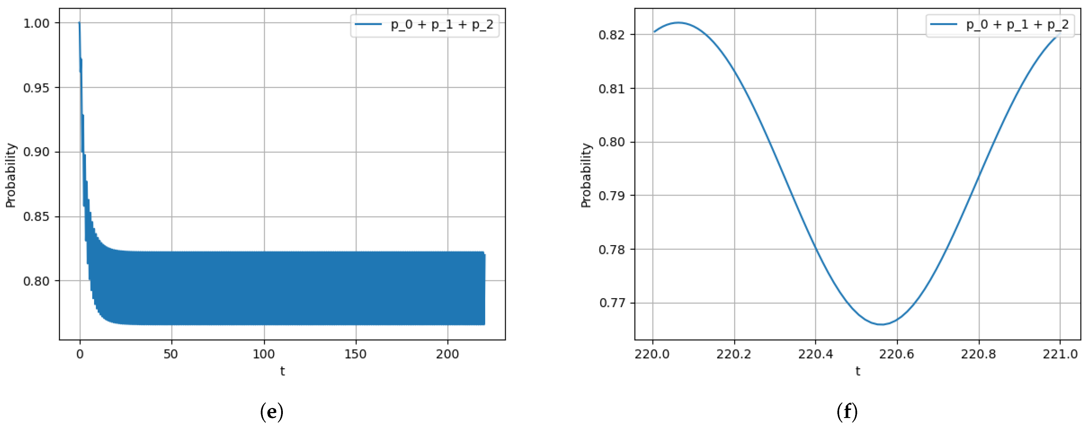
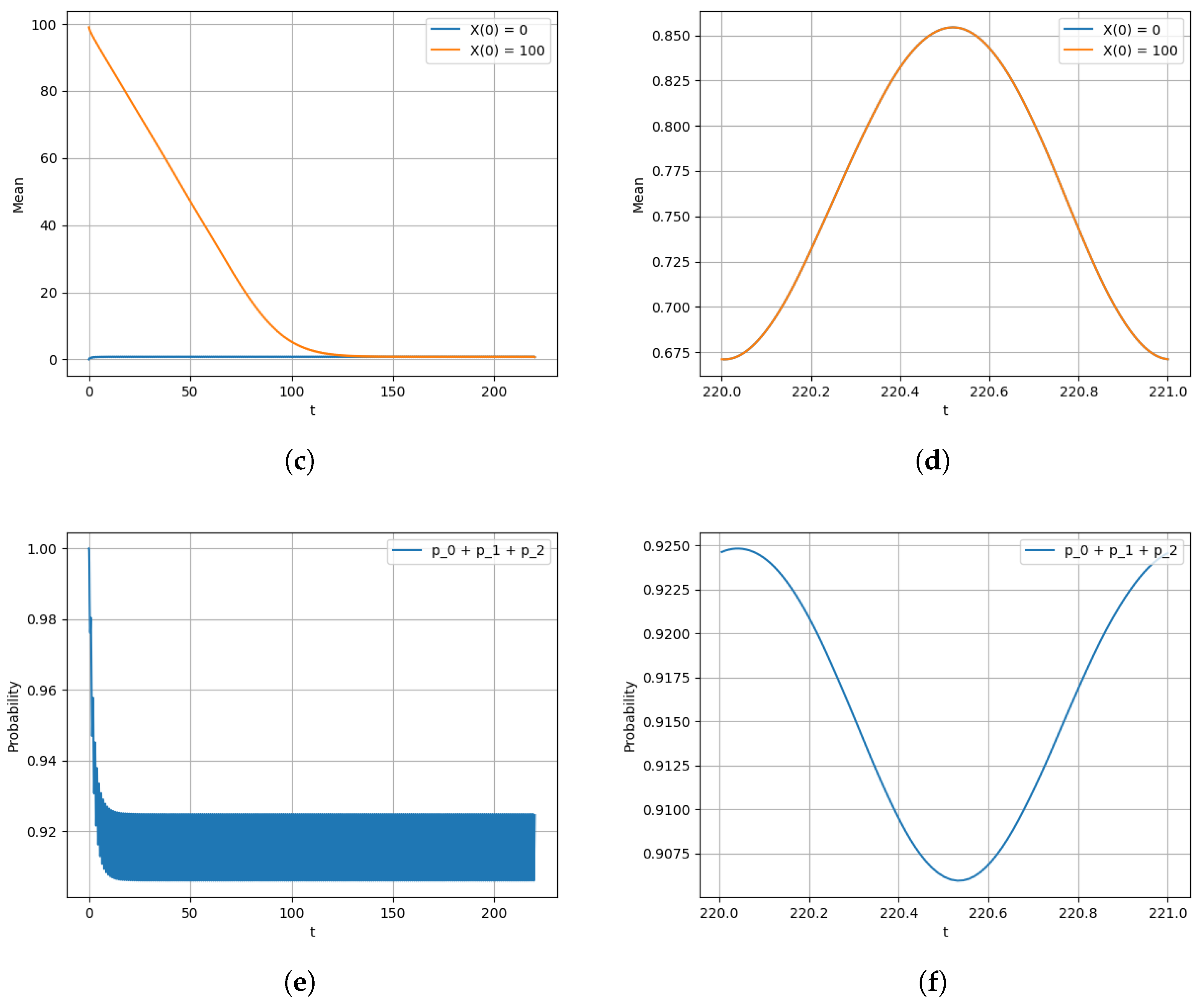
- Let and ; this is a model for the queue with discouragement. Hence, we obtain :Detailed considerations (see [15]) show that it is sufficient to limit ourselves to a truncated BDP with states from 0 to 100. The corresponding graphs are presented in Figure 1.
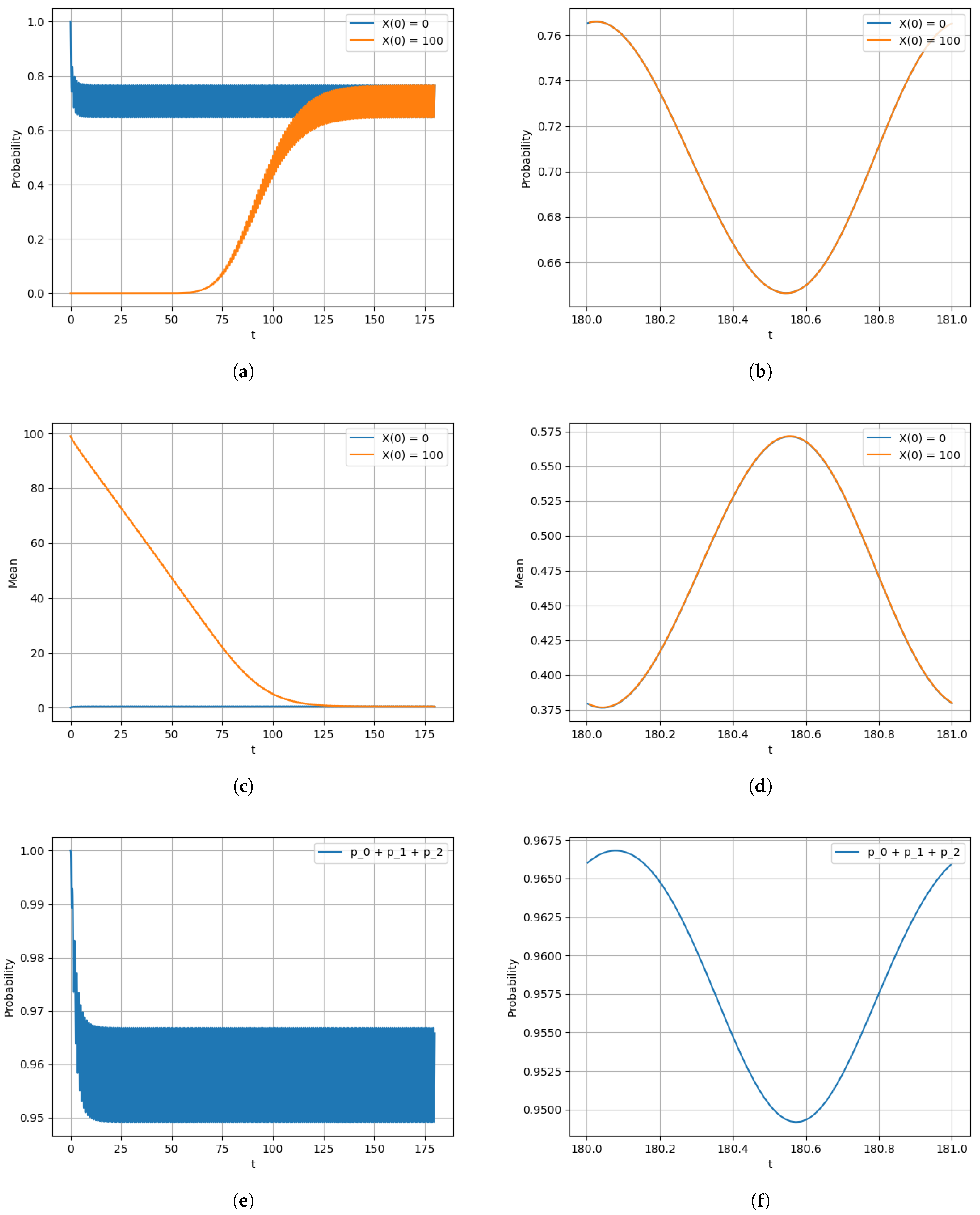
- Let and ; this is a model for the queue with encouragement. Hence, we obtainThe corresponding graphs are shown in Figure 2.
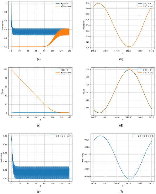
Figure 1.
(a) convergence of the probability under the two different initial conditions: , ; (b) limiting version of the probability under the two different initial conditions: and ; (c) the mean on the interval , where ; (d) the limiting mean on the interval , where ; (e) the probability on the interval ; (f) limiting version of the probability on the interval .
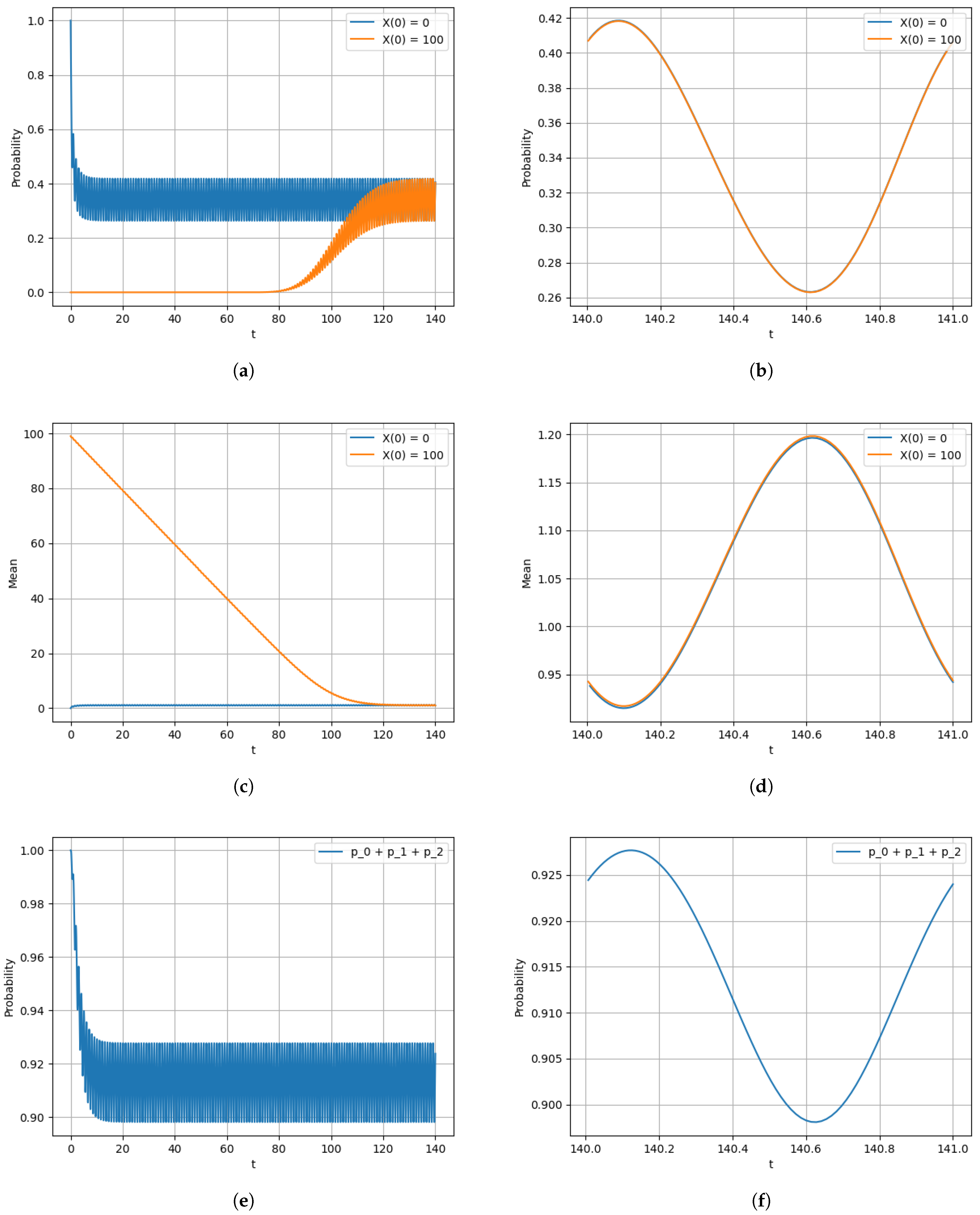
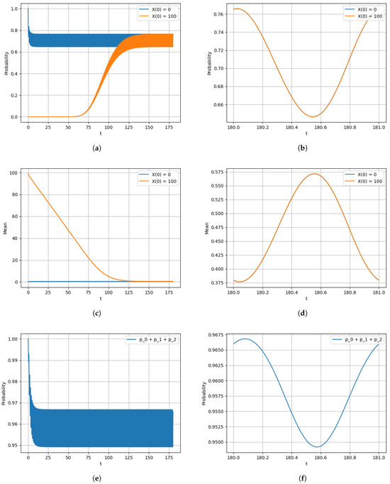
Figure 2.
(a) Convergence of the probability under the two different initial conditions: and ; (b) limiting version of the probability under the two different initial conditions: and ; (c) the mean on the interval , where ; (d) the limiting mean on the interval , where ; (e) the probability on the interval ; (f) the limiting version of the probability on the interval .
- 3.
- Let and ; this is a model for the queue with impatience. Hence, we obtainThe corresponding graphs are shown in Figure 3.
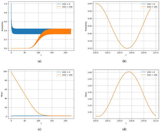

Figure 3.
(a) Convergence of the probability under the two different initial conditions: and ; (b) limiting version of the probability under the two different initial conditions: and ; (c) the mean on the interval , where ; (d) the limiting mean on the interval , where ; (e) the probability on the interval ; (f) the limiting version of the probability on the interval .

- 4.
- Let and ; this is a model with a server that works less effectively as the queue length increases. Hence, we obtainThe corresponding graphs are shown in Figure 4.
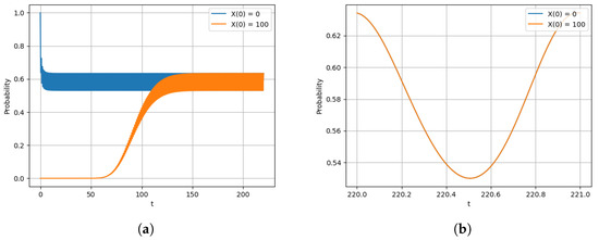
Figure 4.
(a) Convergence of the probability under the two different initial conditions: and ; (b) limiting version of the probability under the two different initial conditions: and ; (c) the mean on the interval , where ; (d) the limiting mean on the interval , where ; (e) the probability on the interval ; (f) the limiting version of the probability on the interval .

4. Conclusions
Possible variants of the simplest models of queueing systems of the type are considered. The queue-length process in such systems is described by a BDP, in which the rates of birth (arrivals) and death (servicing) depend on the behavior of customers and the server. For each queue type, the corresponding specific nonstationary system is considered in the weakly ergodic case. Estimates of the rate of convergence to the limiting regime were obtained. The presence of such estimates provides a guaranteed opportunity to compute the limiting characteristics of the system, and therefore, from [15], we can obtain the corresponding estimates of perturbations and approximations via truncations.
Author Contributions
Conceptualization, supervision, A.Z.; methodology, Y.S.; software, validation, visualization I.U.; investigation, writing, I.U., Y.S., A.Z. and J.S. All authors have read and agreed to the published version of the manuscript.
Funding
This research received no external funding.
Institutional Review Board Statement
Not applicable.
Informed Consent Statement
Not applicable.
Data Availability Statement
Data are contained within the article.
Conflicts of Interest
The authors declare no conflicts of interest.
References
- Natvig, B. On the transient state probabilities for a queueing model where potential customers are discouraged by queue length. J. Appl. Probab. 1974, 11, 345–354. [Google Scholar] [CrossRef]
- Ammar, S.I.; El-Sherbiny, A.A.; El-Shehawy, S.A.; Al-Seedy, R.O. A matrix approach for the transient solution of an M/M/1/N queue with discouraged arrivals and reneging. Int. J. Comput. Math. 2012, 89, 482–491. [Google Scholar] [CrossRef]
- Van Doorn, E.A. The transient state probabilities for a queueing model where potential customers are discouraged by queue length. J. Appl. Probab. 1981, 18, 499–506. [Google Scholar] [CrossRef]
- Reynolds, J.F. The stationary solution of a multiserver queuing model with discouragement. Oper. Res. 1968, 16, 64–71. [Google Scholar] [CrossRef]
- Baccelli, F.; Hebuterne, G. On Queues with Impatient Customers [Research Report] RR-0094. INRIA. 1981. inria-00076467. Available online: https://inria.hal.science/inria-00076467/document (accessed on 1 January 2020).
- Wang, K.; Li, N.; Jiang, Z. Queueing system with impatient customers: A review. In Proceedings of the 2010 IEEE International Conference on Service Operations and Logistics, and Informatics, QingDao, China, 15–17 July 2010; IEEE Xplore: New York, NY, USA, 2010; pp. 82–87. [Google Scholar] [CrossRef]
- Sudhesh, R. Transient analysis of a queue with system disasters and customer impatience. Queueing Syst. 2010, 66, 95–105. [Google Scholar] [CrossRef]
- Dudin, A.N.; Dudin, S.A.; Klimenok, V.I.; Dudina, O.S. Stability of queueing systems with impatience, balking and non-persistence of customers. Mathematics 2024, 12, 2214. [Google Scholar] [CrossRef]
- Jouini, O.; Roubos, A. On multiple priority multi-server queues with impatience. J. Oper. Res. Soc. 2014, 65, 616–632. Available online: https://www.tandfonline.com/doi/abs/10.1057/jors.2012.153 (accessed on 1 January 2020). [CrossRef]
- Puha, A.L.; Ward, A.R. Scheduling an overloaded multiclass many-server queue with impatient customers. In Operations Research & Management Science in the Age of Analytics; INFORMS: Catonsville, MD, USA, 2019; pp. 189–217. Available online: https://pubsonline.informs.org/doi/abs/10.1287/educ.2019.0196 (accessed on 1 January 2020).
- Dong, J.; Ibrahim, R. SRPT scheduling discipline in many-server queues with impatient customers. Manag. Sci. 2021, 67, 7708–7718. Available online: https://pubsonline.informs.org/doi/abs/10.1287/mnsc.2021.4110 (accessed on 1 January 2020). [CrossRef]
- Som, B.K. A Markovian feedback queuing model with encouraged arrivals and customers impatience. In Proceedings of the 2nd International Conference on Evidence Based Management, BITS, Pilani, India, 17–18 March 2017; Available online: https://scholar.google.com/scholar?lookup=0&q=A+Markovian+feedback+queuing+model+with+encouraged+arrivals+and+customers+impatience.&hl=ru&as_sdt=0,5 (accessed on 1 January 2020).
- Som, B.K.; Seth, S. M/M/c/N queuing systems with encouraged arrivals, reneging, retention and feedback customers. Yugosl. J. Oper. Res. 2018, 28, 333–344. [Google Scholar] [CrossRef]
- Ingolfsson, A.; Akhmetshina, E.; Budge, S.; Li, Y.; Wu, X. A survey and experimental comparison of service-level approximation methods for nonstationary M(t)/M/s(t) queueing systems with exhaustive discipline. INFORMS J. Comput. 2007, 19, 149–312. [Google Scholar] [CrossRef]
- Zeifman, A.; Satin, Y.; Korolev, V.; Usov, I. Continuous-time Markov chains and models: Bounding via forward Kolmogorov system. In Handbook of Statistics; Elsevier: Amsterdam, The Netherlands, 2025; Volume 52, pp. 179–210. Available online: https://www.sciencedirect.com/science/article/abs/pii/S0169716125000069 (accessed on 1 June 2025).
- Granovsky, B.L.; Zeifman, A.I. The decay function of nonhomogeneous birth-death processes, with application to mean-field models. Stoch. Proc. Appl. 1997, 72, 105–120. [Google Scholar] [CrossRef]
Disclaimer/Publisher’s Note: The statements, opinions and data contained in all publications are solely those of the individual author(s) and contributor(s) and not of MDPI and/or the editor(s). MDPI and/or the editor(s) disclaim responsibility for any injury to people or property resulting from any ideas, methods, instructions or products referred to in the content. |
© 2025 by the authors. Licensee MDPI, Basel, Switzerland. This article is an open access article distributed under the terms and conditions of the Creative Commons Attribution (CC BY) license (https://creativecommons.org/licenses/by/4.0/).