Open AccessArticle Stability Analysis and Local Convergence of a New Fourth-Order Optimal Jarratt-Type Iterative Scheme by Eulalia MartínezEulalia Martínez SciProfiles Scilit Preprints.org Google Scholar 1, José A. ReyesJosé A. Reyes SciProfiles Scilit Preprints.org Google Scholar 2,3,*, Alicia CorderoAlicia Cordero SciProfiles Scilit Preprints.org Google Scholar 1 and Juan R. TorregrosaJuan R. Torregrosa SciProfiles Scilit Preprints.org Google Scholar 1 1 Multidisciplinary Mathematics Institute, Universitat Politècnica de València (UPV), 46022 Valencia, Spain 2 Departamento de Ciencias Básicas, Instituto Tecnológico de Santo Domingo (INTEC), Santo Domingo 10602, Dominican Republic 3 Escuela de Matemática, Universidad Autónoma de Santo Domingo (UASD), Alma Máter, Santo Domingo 10105, Dominican Republic * Author to whom correspondence should be addressed. Computation 2025, 13(6), 142; https://doi.org/10.3390/computation13060142 Submission received: 17 April 2025 / Revised: 30 May 2025 / Accepted: 3 June 2025 / Published: 9 June 2025 Download keyboard_arrow_down Download PDF Download PDF with Cover Download XML Download Epub Browse Figures Versions Notes Abstract In this work, using the weight function technique, we introduce a new family of fourth-order iterative methods optimal in the sense of Kung and Traub for scalar equations, generalizing Jarratt’s method. Through Taylor series expansions, we confirm that all members of this family achieve fourth-order convergence when derivatives up to the fourth order are bounded. Additionally, a stability analysis is performed on quadratic polynomials using complex discrete dynamics, enabling differentiation among the methods based on their stability. To demonstrate practical applicability, a numerical example illustrates the effectiveness of the proposed family. Extending our findings to Banach spaces, we conduct local convergence analyses on a specific subfamily containing Jarratt’s method, requiring only boundedness of the first derivative. This significantly broadens the method’s applicability to more general spaces and reduces constraints on higher-order derivatives. Finally, additional examples validate the existence and uniqueness of approximate solutions in Banach spaces, provided the initial estimate lies within the locally determined convergence radius obtained using majorizing functions. Keywords: iterative methods; convergence order; nonlinear equations; stability; dynamical plane; nonlinear systems; Banach space; local convergence 1. IntroductionMathematics has become a fundamental tool for addressing applied-world problems in various areas such as physics, engineering, and biology.However, not all situations in the applied world that are solved with a mathematical model can be reduced to an equation with an existing solution formula. For instance, if the mathematical model associated with a problem reduces to a fifth-degree polynomial equation, then it is not possible to find a formula that determines these solutions using only radicals and basic arithmetic operations. This was demonstrated by the mathematician Niels Henrik Abel in 1824. Hence arises the necessity of fixed-point iterative schemes, as they allow us to determine the solutions of equations without the need for a formula. Due to advancements in computer science, these numerical methods have become very popular and highly utilized (see, for example, [1,2,3,4]). They have become a practical and efficient tool due to the computational power and numerical precision of computers, as well as the development of software such as Matlab and Python, which are widely used in numerical computation and iterative methods.Given their versatility, we can use iterative schemes to solve various types of nonlinear equations. However, there are factors that determine whether a method performs better or worse than another in approximating a solution of an equation. One of these factors is its dependence on the initial estimate x 0 . If the function whose zeros we are approximating is not very smooth or if it has multiple possible solutions, it could slow down convergence or converge to a fixed point that is not a solution of the equation, posing a problem of local convergence and numerical sensitivity.Currently, there are several well-behaved numerical methods for approximating solutions to the equation f ( x ) = 0 . However, the applicability of a given iterative scheme depends on whether the assumptions required to guarantee the convergence to an approximate solution are satisfied.Suppose we want to evaluate the suitability of using one of the many derivative-based methods available in the literature to approximate the solution of a given problem f ( x ) = 0 , where f is a scalar function of a real variable. A natural first filter would be to select an iterative method that is optimal in the sense of Kung and Traub [5]. This means that if p is the order of convergence of the method and d is the number of functional evaluations per iteration, the inequality p ≤ 2 d − 1 must be satisfied. The method is said to be optimal when the equality holds.Consider, for example, Newton’s method, defined in [6] as follows: x i + 1 = x i − f ( x i ) f ′ ( x i ) , i = 0 , 1 , … . (1) This iterative scheme satisfies the optimality criterion of Kung and Traub since its order of convergence is 2 and it requires only two functional evaluations per iteration.The proof of this convergence order can be obtained using a Taylor series expansion. For this, it is necessary to impose certain hypotheses on the function f, the solution x ¯ of the problem f ( x ) = 0 , and the initial guess x 0 . Specifically, it is required that the first and second derivatives of f be bounded, that x ¯ be a simple root of f, and that x 0 be sufficiently close to x ¯ . If these conditions are not met, the method may degrade to linear convergence or even fail to converge. In particular, the boundedness of the derivatives is essential for the Taylor-based proof to guarantee the desired convergence order since the error constant depends on those derivatives.Regarding the solution x ¯ , it must be a simple root. Observing the structure of Newton’s method in Equation (1), we note the quotient f ( x i ) f ′ ( x i ) . If x ¯ is a multiple root and x 0 is very close to x ¯ , then f ′ ( x 0 ) will be very small, which may reduce the order of convergence or cause divergence. For this reason, Newton’s method is not recommended for approximating multiple roots.Let us now analyze the restrictions on the initial estimate x 0 . When implementing an iterative scheme such as Newton’s method to approximate a simple root of a scalar function, two stopping criteria are typically established:For some i < n , the condition | x i + 1 − x i | < δ is satisfied. | f ( x i + 1 ) | < ϵ .where n is the maximum number of iterations allowed.If the first condition is met, it implies that x i + 1 is very close to a fixed point or a periodic attractor of the rational operator R f associated with the iterative method. It is known that the roots of f are superattracting fixed points of R f . Therefore, to ensure that the iteration converges to an actual root of f, the second condition | f ( x i + 1 ) | < ϵ is also imposed. This confirms that the orbit generated from x 0 indeed tends to a root of f.If these criteria are not satisfied within n iterations, it may be that x i + 1 lies on a non-attracting periodic orbit or in the stable or unstable manifold of a parabolic fixed point or simply that the method does not reach the desired tolerance with the given initial estimate.This highlights the fact that iterative methods are sensitive to the initial guess and, consequently, exhibit limited numerical stability.At present, there is no known technique capable of constructing a numerical method such that for any initial estimate x 0 , the orbit generated by the method converges to a zero of the function f under consideration. In other words, no method has been developed whose only basins of attraction of the associated rational operator R f are the roots of f. If such a method existed, it would represent a completely stable iterative scheme.This problem remains unresolved for arbitrary functions. However, if f is a quadratic polynomial—the simplest case among nonlinear functions—the behavior of Newton’s method can be analyzed using tools from complex discrete dynamics, particularly through a Möbius transformation.In this context, Blanchard [7] showed that for quadratic polynomials, Newton’s method is stable. This means that it is not sensitive to the initial estimate. Furthermore, it satisfies the Cayley quadratic test, which implies that the only basins of attraction are those corresponding to the roots of the polynomial and that these basins coincide exactly with their immediate basins of attraction.As a consequence, the uniqueness of the solution is guaranteed within each region of the complex plane: if the initial estimate x 0 lies inside the unit circle, the method converges to one root of f; if it lies outside, it converges to the other.Theorem 1 (Cayley quadratic test (CQT)). Let R q ( z ) be the rational operator obtained from a general iteration function applied to the quadratic polynomial q ( z ) = z − a z − b , with a ≠ b . Suppose that R q ( z ) conjugates to the mapping z → z p by the Möbius transformation A ( z ) = z − a z − b . Then, p is the order of method associated to R q ( z ) . Moreover, the corresponding Julia set J ( R q ( z ) ) is the circle S 1 [8].The construction of new numerical methods that improve or enhance the stability of existing methods is a very active line of research. For instance, using the composition technique, it is possible to design a numerical method that doubles the order of convergence of Newton’s method. However, this also doubles the number of functional evaluations per iteration, which prevents the resulting method from being optimal in the sense of Kung and Traub.On the other hand, a common practice in the literature is the construction of parametric families of numerical methods, understood as generalizations of well-known and reliable schemes. In this context, the different members of the family are classified according to their stability when applied to simple functions, such as quadratic polynomials.The motivation for this classification lies in the empirical observation that methods performing well on quadratic functions also tend to exhibit better behavior when applied to more complex functions. In contrast, those that are not stable for such functions generally perform worse when applied to more challenging problems (see, for example, [9,10,11,12,13,14,15], among others).Let us consider the following family of iterative methods: x i + 1 = x i − α f ( x i ) f ′ ( x i ) , i = 0 , 1 , … . (2) This defines a one-parameter family of numerical methods that generalizes Newton’s method, which is recovered when α = 1 . The other members of the family are commonly referred to in the literature as damped Newton methods. None of these damped methods satisfy the optimality criterion of Kung and Traub, as they have an order of convergence less than 2. Therefore, this generalization does not produce new iterative methods that preserve the order or stability of Newton’s method.Next, we introduce Jarratt’s method, which has an order of convergence equal to 4 and requires three functional evaluations per iteration. Thus, it satisfies the optimality criterion of Kung and Traub. Moreover, it is stable when applied to quadratic polynomials. In fact, it exhibits the same stability for these functions as Newton’s method since it also satisfies the Cayley quadratic test.Jarratt’s method, as defined in [16], is given by the following: y i = x i − 2 3 f ( x i ) f ′ ( x i ) , x i + 1 = x i − 1 2 3 f ′ ( y i ) + f ′ ( x i ) 3 f ′ ( y i ) − f ′ ( x i ) f ( x i ) f ′ ( x i ) , i = 0 , 1 , … , (3) where f is a real-valued function of a real variable.If, in the first factor of the subtrahend in the second step, we divide both the numerator and denominator by f ′ ( y i ) , then Jarratt’s method can be rewritten as follows: y i = x i − 2 3 f ( x i ) f ′ ( x i ) , x i + 1 = x i − 3 + f ′ ( x i ) f ′ ( y i ) 6 − 2 f ′ ( x i ) f ′ ( y i ) f ( x i ) f ′ ( x i ) , i = 0 , 1 , … (4) Let us now consider the construction of a two-step method, where the first step corresponds to the family introduced in Equation (2), and the second step is a variant of the composition of this family with itself. Specifically, we define the following: y i = x i − α f ( x i ) f ′ ( x i ) , x i + 1 = x i − α f ( y i ) f ′ ( y i ) , i = 0 , 1 , … (5) It is known that if α = 1 , the resulting method has an order of convergence of 4, but it requires four functional evaluations per iteration. Therefore, it does not satisfy the optimality criterion of Kung and Traub.By examining this iterative scheme, we can observe that if we apply a technique known as the frozen derivative approach, we can avoid introducing new functional evaluations in the second step. This technique consists of freezing the evaluations of f and f ′ in the second step and using their values from the first step.Now, suppose we replace the parameter α in the second step with a weight function H ( x i ) in such a way that only one new evaluation of f ′ ( y i ) is added. In this case, if we define the weight function as H ( x i ) = 3 + f ′ ( x i ) f ′ ( y i ) 6 − 2 f ′ ( x i ) f ′ ( y i ) , then, for α = 2 3 , we recover Jarratt’s method as a combination of three techniques: composition, the frozen derivative, and the use of weight functions.This naturally leads to the question: Are there parameters that allow us to modify the weight function H to thereby generate a new family of fourth-order optimal numerical methods that generalize Jarratt’s method?In this work, we construct a generalization of Jarratt’s method using the weight function technique. We classify the members of this new family based on their stability when applied to quadratic polynomial functions. Specifically, we identify and label as stable those members that exhibit good behavior on such functions.Through empirical examples involving more complex nonlinear functions, we verify that the members of the family which are stable on quadratic polynomials tend to perform better than do the unstable ones when applied to these more challenging cases. Additionally, we compare the performance of the best-performing methods in the family with other well-known methods from the literature and find that they are competitive in terms of accuracy and convergence behavior.In Section 2, we establish the form of the weight function used in the iterative scheme to construct the new family and provide necessary and sufficient conditions on this function to ensure that each member is an optimal method. We also discuss some fundamental properties of the weight function.In Section 3, utilizing discrete complex dynamics, we analyze the stability on quadratic polynomials of each member of the family for the parameters that specialize the method contained within a certain range.In Section 2, we established that if f : Ω ⊂ R ⟶ R is a function with bounded derivatives up to order four and if x ¯ ∈ Ω is a simple root of the equation f ( x ) = 0 , then for an initial estimate x 0 sufficiently close to x ¯ , it is possible to construct a tetraparametric family of optimal iterative methods in the sense of Kung and Traub.This family, for fixed integer values of the parameters, allows us to obtain a numerical method with an order of convergence of four, provided that the hypotheses stated in the previous paragraph are satisfied.Given an iterative scheme, one may ask whether there exist convergence analyses that relax the boundedness conditions imposed on a certain number of derivatives of the scalar function f and whether the method can be reformulated to operate in more general spaces, thereby addressing a wider range of problems. The answer is yes. There are convergence studies—such as local and semi-local convergence analyses—that by imposing appropriate conditions on the function f, the initial estimate x 0 , and the solution x ¯ , allow for a weakening of the standard convergence hypotheses while still guaranteeing the existence and uniqueness of a solution to the problem F ( x ) = 0 , where F is a vector-valued function.Therefore, after constructing the family and analyzing its stability, we extend the applicability of our methods. In particular, for a one-parameter subfamily whose members are all stable when applied to quadratic polynomials, we broaden the theoretical framework by reducing the derivative requirements that were necessary in Section 2 to ensure convergence.In Section 4, with the aim of reducing the boundedness conditions on the derivatives of f up to order four and broadening the scope of application to more general problems, we consider nonlinear systems of equations of the form F ( x ) = 0 , where F : Ω ⊂ X ⟶ Y is a nonlinear, continuous, and twice Fréchet-differentiable operator.Here, Ω is an open and convex set, and X and Y are Banach spaces. In this context, we extend to Banach spaces a subfamily that includes Jarratt’s method. We perform a local convergence analysis without using the Taylor series expansion, which allows us to guarantee the existence and uniqueness of a solution to the problem F ( x ) = 0 , provided that the initial estimate x 0 lies within a convergence radius computed using two majorizing functions, ω 0 : [ 0 , ∞ ) → [ 0 , ∞ ) , ω 1 : [ 0 , ρ 0 ) → [ 0 , ∞ ) , that bind certain conditions imposed on the first derivative of the operator F.Moreover, we obtain a larger convergence radius than those obtained by Argyros in [17] for the two numerical examples presented in this section. 2. Construction of a New Parametric Family of Iterative Jarratt-Type MethodsThe analysis of the applicability of an iterative process requires consideration of two fundamental types of conditions: those associated with the initial guess x 0 , known as accessibility conditions, and those related to the function f. The accessibility of an iterative method can be assessed from three perspectives: the basin of attraction, the region of accessibility, and the parameter domain. The first two perspectives, which are experimental in nature, are linked to the equation f ( x ) = 0 being solved, while the parameter domain, which is theoretical, does not depend on a specific equation but is based on semilocal convergence results applicable to any equation.Regarding convergence, iterative methods can be classified into three main categories: local convergence, which imposes conditions on f and its solution x ¯ ; semilocal convergence, which imposes constraints on f and the initial guess x 0 ; and global convergence, which requires conditions on the function within a defined interval.In this work, we employ the weight function technique to develop a new family of iterative methods optimal in the scalar case, according to Kung and Traub’s conjecture, as a generalization of Jarratt’s method (3).Following reasoning similar to that presented in [14], we establish the necessary and sufficient conditions under which each member of the family achieves fourth-order convergence. We analyze the stability of these methods on quadratic polynomials using complex dynamics. Furthermore, using analogous conditions to those described in [18,19], we extend this scheme to problems in Banach spaces and perform local convergence analyses.As shown in Equation (4), Jarratt’s method can be written as follows: y i = x i − 2 3 f x i f ′ x i , x i + 1 = x i − H ( x i ) f x i f ′ x i , i = 0 , 1 , … , (6) where H ( x i ) = 3 + f ′ x i f ′ y i 6 − 2 f ′ x i f ′ y i . With μ ( x i ) = f ′ x i f ′ y i , it follows that Jarratt’s method belongs to a family of iterative schemes of the form (6), where H ( x ) is a weight function with the following general structure: H ( x ) = s μ ( x ) k + q μ ( x ) g n μ ( x ) l + m μ ( x ) w . The following result provides the necessary and sufficient conditions that H ( x ) must satisfy for the iterative scheme members of this family. y i = x i − 2 3 f x i f ′ x i , x i + 1 = x i − s μ ( x i ) k + q μ ( x i ) g n μ ( x i ) l + m μ ( x i ) w f x i f ′ x i , i = 0 , 1 , … , (7) are optimal fourth-order methods.Theorem 2. Let f : Ω ⊂ R ⟶ R be a sufficiently differentiable function and let x ¯ ∈ Ω be a simple root of the equation f ( x ) = 0 . Then the method (7) has an order of convergence of 4 if and only if the following conditions hold: g ≠ k , l ≠ w , − 4 l ( g + k ) + g ( 4 k − 3 ) − 3 k + 4 l 2 + 6 l + 6 ≠ 0 , and H ( x ) = H 1 ( x ) if λ = l and δ 1 = β 1 H 2 ( x ) if λ = l and δ 1 ≠ β 1 H 3 ( x ) if λ = k and δ 1 ≠ β 1 , where λ = min { δ 1 , β 1 } , δ 1 = min { k , g } , β 1 = min { l , w } , H 1 ( x ) = w 8 g 2 − 4 g ( 2 w + 3 ) + 6 w − 3 − w ( 6 w − 3 ) μ ( x ) g − λ 2 g ( g ( 4 w + 3 ) − 2 w ( 2 w + 3 ) − 6 ) + 2 ( 6 − 3 g ) g μ ( x ) w − λ , H 2 ( x ) = w 8 g 2 − 4 g ( 2 w + 3 ) + 6 w − 3 μ ( x ) k − λ − w 8 k 2 − 4 k ( 2 w + 3 ) + 6 w − 3 μ ( x ) g − λ 2 ( g − k ) ( g ( − 4 k + 4 w + 3 ) + k ( 4 w + 3 ) − 2 w ( 2 w + 3 ) − 6 ) + 2 ( g − k ) ( g ( 4 k − 3 ) − 3 k + 6 ) μ ( x ) w − λ , H 3 ( x ) = ( w − l ) 8 g 2 − 4 g ( 2 l + 2 w + 3 ) + l ( 8 w + 6 ) + 6 w − 3 + ( l − w ) ( l ( 8 w + 6 ) + 6 w − 3 ) μ ( x ) g − λ 2 g ( g ( 4 w + 3 ) − 2 w ( 2 w + 3 ) − 6 ) μ ( x ) l − λ + 2 g − 4 g l − 3 g + 4 l 2 + 6 l + 6 μ ( x ) w − λ , and the error equation is given by e i + 1 = c 2 3 G 1 − G 2 + G 3 + G 4 − c 3 c 2 + c 4 9 e i 4 + O e i 5 , where G 1 = 8 g 2 8 k 2 − 4 k ( 2 l + 2 w + 3 ) + l ( 8 w + 6 ) + 6 w − 3 81 ( 2 g + 2 k − 2 l − 2 w − 3 ) , G 2 = 2 g 16 k 2 ( 2 l + 2 w + 3 ) − 4 k 8 l 2 + 8 l ( 2 w + 3 ) + 8 w 2 + 24 w + 33 + 8 l 2 ( 4 w + 3 ) + N 81 ( 2 g + 2 k − 2 l − 2 w − 3 ) , G 3 = 8 k 2 ( l ( 8 w + 6 ) + 6 w − 3 ) − 2 k 8 l 2 ( 4 w + 3 ) + N 81 ( 2 g + 2 k − 2 l − 2 w − 3 ) , G 4 = 64 l 2 w 2 + 96 l 2 w + 96 l 2 + 96 l w 2 + 24 l w − 210 l + 96 w 2 − 210 w − 207 81 ( 2 g + 2 k − 2 l − 2 w − 3 ) , and N = l 32 w 2 + 96 w + 54 + 3 8 w 2 + 18 w − 35 .Proof. Applying the Taylor series expansion of f ( x i ) around x ¯ , we obtain the following: f ( x i ) = f ( x ¯ ) + f ′ ( x ¯ ) ( x i − x ¯ ) + f ″ ( x ¯ ) 2 ! ( x i − x ¯ ) 2 + f ‴ ( x ¯ ) 3 ! ( x i − x ¯ ) 3 + f ( 4 ) ( x ¯ ) 4 ! ( x i − x ¯ ) 4 + O ( x i − x ¯ ) 5 , (8) Since x ¯ is assumed to be a simple zero of f ( x ) , it follows that f ( x ¯ ) = 0 and f ′ ( x ¯ ) ≠ 0 . Therefore, the function f ( x i ) can be written as follows: f ( x i ) = f ′ ( x ¯ ) e i + c 2 e i 2 + c 3 e i 3 + c 4 e i 4 + O e i 5 , (9) where c j = 1 j ! f ( j ) ( x ¯ ) f ′ ( x ¯ ) , j = 2 , 3 , … , e i = x i − x ¯ . Consequently, f ′ ( x i ) = f ′ ( x ¯ ) 1 + 2 c 2 e i + 3 c 3 e i 2 + 4 c 4 e i 3 + O e i 4 . (10) Dividing directly (9) by (10), we obtain f ( x i ) f ′ ( x i ) = e i − c 2 e i 2 + 2 c 2 2 − c 3 e i 3 − 4 c 2 3 − 7 c 2 c 3 + 3 c 4 e i 4 + O e i 5 . Subtracting x ¯ from both sides gives the error expression y i − x ¯ = e i − 2 3 f ( x i ) f ′ ( x i ) = 1 3 e i + 2 3 c 2 e i 2 + 4 3 c 3 − c 2 2 e i 3 + 2 3 4 c 2 3 − 7 c 2 c 3 + 3 c 4 e i 4 + O e i 5 . Then, f ′ ( y i ) = 1 + 2 3 c 2 e i + 1 3 4 c 2 2 + c 3 e i 2 + 4 27 − 18 c 2 3 + 27 c 3 c 2 + c 4 e i 3 + O e i 4 . (11) Dividing (10) by (11), we have μ ( x ) = f ′ ( x i ) f ′ ( y i ) = 1 + 4 3 c 2 e i + 4 9 6 c 3 − 5 c 2 2 e i 2 + 8 27 8 c 2 3 − 21 c 3 c 2 + 13 c 4 e i 3 + O e i 4 , H ( x i ) = q + s m + n + F 1 e i + 4 F 2 + F 3 9 ( m + n ) e i 2 + 8 F 4 + F 5 + F 6 − q + s ( m + n ) 3 2 F 7 + F 8 c 2 3 − F 9 + F 10 81 ( m + n ) e i 3 + O e i 4 , F 1 = 4 c 2 ( g q ( m + n ) + k m s + k n s − l n ( q + s ) − m q w − m s w ) 3 ( m + n ) 2 , F 2 = − 4 c 2 2 ( g q + k s ) ( l n + m w ) m + n + g q c 2 2 ( 2 g − 7 ) + 6 c 3 + k s c 2 2 ( 2 k − 7 ) + 6 c 3 , F 3 = ( q + s ) c 2 2 2 l 2 n ( n − m ) + l n ( m ( 8 w + 7 ) + 7 n ) + m w ( m ( 2 w + 7 ) + n ( 7 − 2 w ) ) − 6 c 3 ( m + n ) ( l n + m w ) ( m + n ) 2 , F 4 = − 6 c 2 ( l n + m w ) c 2 2 2 g 2 q − 7 g q + k ( 2 k − 7 ) s + 6 c 3 ( g q + k s ) m + n , F 5 = 6 c 2 ( g q + k s ) c 2 2 2 l 2 n ( n − m ) + l n ( m ( 8 w + 7 ) + 7 n ) + m w ( m ( 2 w + 7 ) + n ( 7 − 2 w ) ) − 6 c 3 ( m + n ) ( l n + m w ) ( m + n ) 2 , F 6 = g q c 2 3 4 g 2 − 42 g + 62 + 9 c 3 c 2 ( 4 g − 11 ) + 39 c 4 + k s c 2 3 4 k 2 − 42 k + 62 + 9 c 3 c 2 ( 4 k − 11 ) + 39 c 4 , F 7 = 2 l 3 n m 2 − 4 m n + n 2 + m w m 2 2 w 2 + 21 w + 31 + m n 62 − 8 w 2 + n 2 2 w 2 − 21 w + 31 , F 8 = 3 l 2 n − m 2 ( 4 w + 7 ) + 8 m n w + 7 n 2 + l n m 2 24 w 2 + 84 w + 31 + 2 m n − 6 w 2 + 42 w + 31 + 31 n 2 , F 9 = 9 c 2 c 3 ( m + n ) 4 l 2 n ( n − m ) + l n ( m ( 16 w + 11 ) + 11 n ) + m w ( m ( 4 w + 11 ) + n ( 11 − 4 w ) ) , F 10 = 39 c 4 ( m + n ) 2 ( l n + m w ) . Subtracting x ¯ from both sides of the second step of (7), we obtain e i + 1 = 1 − q + s m + n e i + c 2 F 11 e i 2 + 1 9 ( m + n ) 2 F 12 − 4 ( m + n ) F 13 + F 14 e i 3 + O e i 4 , (12) where F 11 = − 4 g q ( m + n ) − 4 k m s − 4 k n s + 4 l n ( q + s ) + 3 ( m + n ) ( q + s ) + 4 m q w + 4 m s w 3 ( m + n ) 2 , F 12 = 12 c 2 2 ( g q ( m + n ) + k m s + k n s − l n ( q + s ) − m q w − m s w ) − 18 c 2 2 − c 3 ( m + n ) ( q + s ) , F 13 = − 4 c 2 2 ( g q + k s ) ( l n + m w ) m + n + g q c 2 2 ( 2 g − 7 ) + 6 c 3 + k s c 2 2 ( 2 k − 7 ) + 6 c 3 , F 14 = ( q + s ) c 2 2 M 1 − 6 c 3 ( m + n ) ( l n + m w ) ( m + n ) 2 , and M 1 = 2 l 2 n ( n − m ) + l n ( m ( 8 w + 7 ) + 7 n + m w ( m ( 2 w + 7 ) + n ( 7 − 2 w ) ) ) . To ensure the error is of order 4, it is necessary that 1 − q + s m + n = 0 , − 4 g q ( m + n ) − 4 k m s − 4 k n s + 4 l n ( q + s ) + 3 ( m + n ) ( q + s ) + 4 m q w + 4 m s w 3 ( m + n ) 2 = 0 , F 15 + 4 ( m + n ) ( F 16 + F 17 ) 9 ( m + n ) 2 = 0 , 18 ( m + n ) ( q + s ) − 4 ( m + n ) 6 g q + 6 k s + ( q + s ) ( − 6 ( m + n ) ( l n + m w ) ) ( m + n ) 2 9 ( m + n ) 2 = 0 , where F 15 = 12 ( g q ( m + n ) + k m s + k n s − l n ( q + s ) − m q w − m s w ) − 18 ( m + n ) ( q + s ) , F 16 = − 4 ( g q + k s ) ( l n + m w ) m + n + g ( 2 g − 7 ) q + k ( 2 k − 7 ) s , F 17 = ( q + s ) 2 l 2 n ( n − m ) + l n ( m ( 8 w + 7 ) + 7 n ) + m w ( m ( 2 w + 7 ) + n ( 7 − 2 w ) ) ( m + n ) 2 . Solving this system for the variables m , n , s , q , we obtain s = − ω ( l − w ) 8 g 2 − 4 g ( 2 l + 2 w + 3 ) + l ( 8 w + 6 ) + 6 w − 3 2 ( g − k ) − 4 l ( g + k ) + g ( 4 k − 3 ) − 3 k + 4 l 2 + 6 l + 6 , q = ω ( l − w ) 8 k 2 − 4 k ( 2 l + 2 w + 3 ) + l ( 8 w + 6 ) + 6 w − 3 2 ( g − k ) − 4 l ( g + k ) + g ( 4 k − 3 ) − 3 k + 4 l 2 + 6 l + 6 , n = ω g ( − 4 k + 4 w + 3 ) + k ( 4 w + 3 ) − 2 w ( 2 w + 3 ) − 6 − 4 l ( g + k ) + g ( 4 k − 3 ) − 3 k + 4 l 2 + 6 l + 6 , m = ω , where ω ∈ R . Note that from the forms of the expressions for s and q, we have g ≠ k and − 4 l ( g + k ) + g ( 4 k − 3 ) − 3 k + 4 l 2 + 6 l + 6 ≠ 0 , and from the equation 1 − q + s m + n = 0 , it follows that l ≠ w , m ≠ 0 and that 8 g 2 − 4 g ( 2 l + 2 w + 3 ) + l ( 8 w + 6 ) + 6 w − 3 ≠ 8 k 2 − 4 k ( 2 l + 2 w + 3 ) + l ( 8 w + 6 ) + 6 w − 3 . Since g ≠ k , the equality 8 g 2 − 4 g ( 2 l + 2 w + 3 ) + l ( 8 w + 6 ) + 6 w − 3 = 8 k 2 − 4 k ( 2 l + 2 w + 3 ) + l ( 8 w + 6 ) + 6 w − 3 holds only if both sides are simultaneously zero.Note that if 8 g 2 − 4 g ( 2 l + 2 w + 3 ) + l ( 8 w + 6 ) + 6 w − 3 = 0 , then g = ( 2 l + 2 w + 3 ) ± ( 2 l + 2 w + 3 ) 2 − 2 l ( 8 w + 6 ) + 6 w − 3 4 , and thus 4 g − ( 2 l + 2 w + 3 ) 2 = ( 2 l + 2 w + 3 ) 2 − 2 l ( 8 w + 6 ) + 6 w − 3 . Expanding and simplifying gives 16 g 2 − 8 g ( 2 l + 2 w + 3 ) = − 16 l w − 12 l − 12 w + 6 , which further simplifies to 8 g 2 − 4 g ( 2 l + 2 w + 3 ) = − 8 l w − 6 l − 6 w + 3 . This equation has no integer solution because the left-hand side is even, while the right-hand side is odd. Therefore, since g is integer, the equation 8 g 2 − 4 g ( 2 l + 2 w + 3 ) + l ( 8 w + 6 ) + 6 w − 3 = 8 k 2 − 4 k ( 2 l + 2 w + 3 ) + l ( 8 w + 6 ) + 6 w − 3 has no solution. Hence, 8 g 2 − 4 g ( 2 l + 2 w + 3 ) + l ( 8 w + 6 ) + 6 w − 3 ≠ 8 k 2 − 4 k ( 2 l + 2 w + 3 ) + l ( 8 w + 6 ) + 6 w − 3 , ∀ k , g , l , w ∈ Z . Now, H ( x ) = s μ ( x ) k + q μ ( x ) g n μ ( x ) l + m μ ( x ) w can be rewritten as H ( x ) = s 1 μ ( x ) k + q 1 μ ( x ) g n 1 μ ( x ) l + m 1 μ ( x ) w , where s 1 ( g , l , w ) = − ( l − w ) 8 g 2 − 4 g ( 2 l + 2 w + 3 ) + l ( 8 w + 6 ) + 6 w − 3 , q 1 ( k , l , w ) = ( l − w ) 8 k 2 − 4 k ( 2 l + 2 w + 3 ) + l ( 8 w + 6 ) + 6 w − 3 , n 1 ( k , g , w ) = 2 ( g − k ) ( g ( − 4 k + 4 w + 3 ) + k ( 4 w + 3 ) − 2 w ( 2 w + 3 ) − 6 ) , m 1 ( k , g , l ) = − 2 ( g − k ) ( g ( − 4 k + 4 l + 3 ) + k ( 4 l + 3 ) − 2 l ( 2 l + 3 ) − 6 ) , for ω ≠ 0 , g ≠ k , and − 4 l ( g + k ) + g ( 4 k − 3 ) − 3 k + 4 l 2 + 6 l + 6 ≠ 0 .Evaluating H ( x ) at μ ( x ) = f ′ ( x i ) f ′ ( y i ) = 1 + 4 3 c 2 e i + 4 9 6 c 3 − 5 c 2 2 e i 2 + 8 27 8 c 2 3 − 21 c 3 c 2 + 13 c 4 e i 3 + O e i 4 , and recalculating the error, we have e i + 1 = c 2 3 G 1 − G 2 + G 3 + G 4 − c 3 c 2 + c 4 9 e i 4 , where c j = 1 j ! f ( j ) ( x ¯ ) f ′ ( x ¯ ) , j = 2 , 3 , … , e i = x i − x ¯ , G 1 = 8 g 2 8 k 2 − 4 k ( 2 l + 2 w + 3 ) + l ( 8 w + 6 ) + 6 w − 3 81 ( 2 g + 2 k − 2 l − 2 w − 3 ) , G 2 = 2 g 16 k 2 ( 2 l + 2 w + 3 ) − 4 k 8 l 2 + 8 l ( 2 w + 3 ) + 8 w 2 + 24 w + 33 + 8 l 2 ( 4 w + 3 ) + N 81 ( 2 g + 2 k − 2 l − 2 w − 3 ) , G 3 = 8 k 2 ( l ( 8 w + 6 ) + 6 w − 3 ) − 2 k 8 l 2 ( 4 w + 3 ) + N 81 ( 2 g + 2 k − 2 l − 2 w − 3 ) , G 4 = 64 l 2 w 2 + 96 l 2 w + 96 l 2 + 96 l w 2 + 24 l w − 210 l + 96 w 2 − 210 w − 207 81 ( 2 g + 2 k − 2 l − 2 w − 3 ) , N = l 32 w 2 + 96 w + 54 + 3 8 w 2 + 18 w − 35 . If in H ( x ) = s 1 μ ( x ) k + q 1 μ ( x ) g n 1 μ ( x ) l + m 1 μ ( x ) w , we simultaneously interchange k and g in s 1 ( g , l , w ) , q 1 ( k , l , w ) , n 1 ( k , g , w ) , and m 1 ( k , g , l ) , then s 1 ( k , l , w ) = − q 1 ( k , l , w ) , q 1 ( g , l , w ) = − s 1 ( g , l , w ) , n 1 ( g , k , w ) = − n 1 ( k , g , w ) , m 1 ( g , k , l ) = − m 1 ( k , g , l ) , and thus H ( g , k , l , w ) ( x ) = s 1 ( k , l , w ) μ ( x ) g + q 1 ( g , l , w ) μ ( x ) k n 1 ( g , k , w ) μ ( x ) l + m 1 ( g , k , l ) μ ( x ) w = − q 1 ( k , l , w ) μ ( x ) g − s 1 ( g , l , w ) μ ( x ) k − n 1 ( k , g , w ) μ ( x ) l − m 1 ( k , g , l ) μ ( x ) w = s 1 ( g , l , w ) μ ( x ) k + q 1 ( k , l , w ) μ ( x ) g n 1 ( k , g , w ) μ ( x ) l + m 1 ( k , g , l ) μ ( x ) w = H ( k , g , l , w ) ( x ) . Similarly, H ( k , g , w , l ) ( x ) = s 1 ( g , w , l ) μ ( x ) k + q 1 ( k , w , l ) μ ( x ) g n 1 ( k , g , l ) μ ( x ) w + m 1 ( k , g , w ) μ ( x ) l = − s 1 ( g , l , w ) μ ( x ) k − q 1 ( k , l , w ) μ ( x ) g − m 1 ( k , g , l ) μ ( x ) w − n 1 ( k , g , w ) μ ( x ) l = s 1 ( g , l , w ) μ ( x ) k + q 1 ( k , l , w ) μ ( x ) g n 1 ( k , g , w ) μ ( x ) l + m 1 ( k , g , l ) μ ( x ) w = H ( k , g , l , w ) ( x ) . Combining these two equations and setting δ 1 = min { k , g } , δ 2 = max { k , g } , β 1 = min { w , l } , and β 2 = max { w , l } , we obtain H ( k , g , w , l ) ( x ) = H ( δ 1 , δ 2 , β 1 , β 2 ) ( x ) . Given that H ( δ 1 , δ 2 , β 1 , β 2 ) ( x ) = s 1 ( δ 2 , β 1 , β 2 ) μ ( x ) δ 1 + q 1 ( δ 1 , β 1 , β 2 ) μ ( x ) δ 2 n 1 ( δ 1 , δ 2 , β 2 ) μ ( x ) β 1 + m 1 ( δ 1 , δ 2 , β 1 ) μ ( x ) β 2 = s 1 ( δ 2 , β 1 , β 2 ) μ ( x ) δ 1 − λ + q 1 ( δ 1 , β 1 , β 2 ) μ ( x ) δ 2 − λ n 1 ( δ 1 , δ 2 , β 2 ) μ ( x ) β 1 − λ + m 1 ( δ 1 , δ 2 , β 1 ) μ ( x ) β 2 − λ = s 1 ( δ 2 − λ , β 1 − λ , β 2 − λ ) μ ( x ) δ 1 − λ + q 1 ( δ 1 − λ , β 1 − λ , β 2 − λ ) μ ( x ) δ 2 − λ n 1 ( δ 1 − λ , δ 2 − λ , β 2 − λ ) μ ( x ) β 1 − λ + m 1 ( δ 1 − λ , δ 2 − λ , β 1 − λ ) μ ( x ) β 2 − λ , if λ = min { δ 1 , β 1 } , then the set { H ( k , g , l , w ) ( x ) } = { H ( 0 , g , l , w ) ( x ) } ∪ { H ( k , g , 0 , w ) ( x ) } , where { H ( 0 , g , l , w ) ( x ) } ∩ { H ( k , g , 0 , w ) ( x ) } = { H ( 0 , g , 0 , w ) ( x ) } , and H ( x ) = H 1 ( x ) if λ = l and δ 1 = β 1 H 2 ( x ) if λ = l and δ 1 ≠ β 1 H 3 ( x ) if λ = k and δ 1 ≠ β 1 . □In the previous theorem, we determined the values of s, q, n, and m as functions of the integer exponents k, g, l, and w such that the members of the family introduced in Equation (7) achieve a convergence order of 4. Additionally, we established conditions that allow for the identification of distinct iterative methods by grouping equivalent weight functions under simplification.In the following section, we perform a stability analysis on quadratic polynomials for those family members where the exponents k, g, l, and w are integers in the range from 0 to 5. Subsequently, we carry out a numerical comparison between the stable and unstable methods using more complex test functions. Finally, we compare the best-performing methods on these functions with the methods of Kung and Traub [5], Chun [20], and Ostrowski [21]. 3. Complex Stability AnalysisThe dynamical study of iterative methods aims to understand the behavior of orbits generated by successive iterations of an operator T f in the complex plane, particularly in the numerical solution of equations of the form f ( z ) = 0 . Determining suitable initial points to ensure convergence toward a specific solution has long been an important question within the mathematical community and remains an active field of research with many open problems. Given z 0 ∈ C ^ , we define the orbit of z 0 under R to be the sequence of points z 0 , z 1 = R ( z 0 ) , z 2 = R 2 ( z 0 ) , … , z n = R n ( z 0 ) , … , where z 0 is called the seed of the orbit. There are many different kinds of orbits, such as the orbit of a fixed point, which is a point z 0 such that R ( z 0 ) = z 0 , the orbit of a periodic point or cycle, where a point z 0 is called n-periodic if R n ( z 0 ) = z 0 for some n > 0 , with R p ( z 0 ) ≠ z 0 for any p < n , and the least such n is called the prime period of the orbit. The stability of a fixed point is determined by | R ′ ( z 0 ) | : z 0 is attracting if | R ′ ( z 0 ) | < 1 , repelling if | R ′ ( z 0 ) | > 1 , and neutral if | R ′ ( z 0 ) | = 1 (see the text by Devaney [22]). Now, suppose z 0 is an attracting fixed point for R; the basin of attraction of z 0 is the set of all points whose orbits tend to z 0 , and the immediate basin of attraction is the largest convex component containing z 0 that lies within the basin. Let x ¯ be a solution of the equation f ( z ) = 0 . A key issue is characterizing the region of the complex plane known as the basin of attraction of the root x ¯ . Its analysis makes it possible to investigate into whether these basins cover the entire complex plane or if there exist areas where the iterative process does not converge to any solution. Depending on the dynamics of the iterative method, various scenarios can be observed: orbits converging to a fixed point solution, coinciding with a root of f ( z ) = 0 ; orbits converging to strange fixed points, which are not solutions but reveal additional structures; periodic orbits or cycles, where a point returns to its position after a finite number of iterations; orbits approaching a cycle without reaching it, exhibiting asymptotic attraction; and chaotic orbits, showing no recognizable patterns.The efficiency of a numerical method depends not only on its convergence order or computational cost per iteration but also on its numerical stability. Thus, the study of complex discrete dynamics becomes an essential tool for evaluating the behavior and reliability of iterative methods applied to solving nonlinear equations. Blanchard and Devaney [22,23] introduced concepts that facilitate stability analysis of multi-step methods for quadratic polynomials, aiding in the identification of dynamical patterns and the selection of the most stable schemes.A rational operator is defined as R ( z ) = P ( z ) Q ( z ) over the Riemann sphere, where P and Q are complex polynomials with no common factors. Analyzing this rational operator induces the study method’s stability and the location of fixed points. Critical points are identified by the condition R ′ ( z C ) = 0 , providing insights into the sensitivity of the operator, and a critical point is called free if it does not coincide with the roots of the polynomial. The basins of attraction include points whose orbits converge to an attracting point, and their union constitutes the Fatou set, whereas the Julia set corresponds to its complementary set in the Riemann sphere [23].The dynamical plane visually illustrates the behavior of the method, revealing basins associated with roots and, in cases of instability, additional basins related to undesired points. Finally, analytic conjugation, introduced by Blanchard [7], enables dynamical analysis through Möbius transformations, facilitating the study of rational operators in an equivalent system where roots are normalized.The following result demonstrates that the family of iterative schemes (7) satisfies the scaling theorem, allowing us to apply Möbius transformations as analytic conjugation. This simplifies the stability analysis of the family members.Theorem 3. Let f ( z ) be an analytic function and A ( z ) = η z + β , with η ≠ 0 , an affine transformation. Let h ( z ) = λ ( f ∘ A ) ( z ) . Then, the fixed-point operators R f and R h of the iterative method (7) are analytically conjugated by A ( z ) .Proof. Let N f ( z ) = z − 2 3 f ( z ) f ′ ( z ) and consider that A ( x − y ) = η ( x − y ) + β = ( η x + β ) − ( η y + β ) + β = A ( x ) − A ( y ) + β . Also, h ( z ) = λ ( f ∘ A ) ( z ) = λ f ( A ( z ) ) ; thus, h ′ ( z ) = A ′ ( z ) λ f ′ ( A ( z ) ) = η λ ( f ′ ∘ A ) ( z ) .Therefore, ( A ∘ N h ∘ A − 1 ) ( z ) = A A − 1 ( z ) − 2 3 h A − 1 ( z ) h ′ A − 1 ( z ) = A A − 1 ( z ) − 2 3 f ( z ) η f ′ ( z ) = z − 2 3 f ( z ) f ′ ( z ) = N f ( z ) . Thus, N f ( z ) and N h ( z ) are analytically conjugated by A ( z ) .Then, R h ( z ) = z − s h ′ ( z ) h ′ ( N h ) k + q h ′ ( z ) h ′ ( N h ) g n h ′ ( z ) h ′ ( N h ) l + m h ′ ( z ) h ′ ( N h ) w h ( z ) h ′ ( z ) . Hence, h ( z ) = λ ( f ∘ A ) ( z ) = λ f ( A ( z ) ) , h ′ ( z ) = η λ ( f ′ ∘ A ) ( z ) , and thus h ′ ( N h ) = η λ ( f ′ ∘ A ∘ N h ) ( z ) . Then, R h ( z ) = z − s f ′ ∘ A f ′ ∘ A ∘ N h k + q f ′ ∘ A f ′ ∘ A ∘ N h g n f ′ ∘ A f ′ ∘ A ∘ N h l + m f ′ ∘ A f ′ ∘ A ∘ N h w 1 η f ∘ A f ′ ∘ A . As ( A ∘ N h ∘ A − 1 ) ( z ) = N f ( z ) , ( R h ∘ A − 1 ) ( z ) = A − 1 ( z ) − s f ′ ( z ) f ′ ∘ N f k + q f ′ ( z ) f ′ ∘ N f g n f ′ ( z ) f ′ ∘ N f l + m f ′ ( z ) f ′ ∘ N f w 1 η f ( z ) f ′ ( z ) , thus ( A ∘ R h ∘ A − 1 ) ( z ) = A A − 1 ( z ) − s f ′ ( z ) f ′ ∘ N f k + q f ′ ( z ) f ′ ∘ N f g n f ′ ( z ) f ′ ∘ N f l + m f ′ ( z ) f ′ ∘ N f w 1 η f ( z ) f ′ ( z ) . Finally, since A ( x − y ) = A ( x ) − A ( y ) + β , it follows that ( A ∘ R h ∘ A − 1 ) ( z ) = z − s f ′ ( z ) f ′ ∘ N f k + q f ′ ( z ) f ′ ∘ N f g n f ′ ( z ) f ′ ∘ N f l + m f ′ ( z ) f ′ ∘ N f w f ( z ) f ′ ( z ) = R f ( z ) , and thus R f ( z ) and R h ( z ) are analytically conjugated by A ( z ) . □If we apply the Möbius transformation A ( u ) = u − a u − b satisfying A ( ∞ ) = 1 , A ( a ) = 0 and A ( b ) = ∞ using conjugation with p ( z ) = ( z − a ) ( z − b ) , where a , b ∈ C , to the iterative scheme (7), we obtain the associated rational operator R h ( z , k , g , l , w ) = A ∘ R p ( z , k , g , l , w , a , b ) ∘ A − 1 . The transformation holds where R p is given by the following: R p ( z , k , g , l , w , a , b ) = ( z − a ) ( z − b ) ( l − w ) 2 ( g − k ) ( a + b − 2 z ) · N ( z ) D ( z ) + z with N ( z ) = 3 g A g S ( z ) g − 3 k A k S ( z ) k , D ( z ) = 3 w B w S ( z ) w + 3 l B l S ( z ) l , S ( z ) = ( a + b − 2 z ) 2 3 a 2 + 2 a ( b − 4 z ) + 3 b 2 − 8 b z + 8 z 2 , and the coefficients defined as A g = 8 k 2 − 4 k ( 2 l + 2 w + 3 ) + l ( 8 w + 6 ) + 6 w − 3 , A k = 8 g 2 − 4 g ( 2 l + 2 w + 3 ) + l ( 8 w + 6 ) + 6 w − 3 , B w = − 4 l ( g + k ) + g ( 4 k − 3 ) − 3 k + 4 l 2 + 6 l + 6 , B l = g ( − 4 k + 4 w + 3 ) + k ( 4 w + 3 ) − 2 w ( 2 w + 3 ) − 6 . Thus, R h takes the form R h ( z , k , g , l , w ) = z · U ( z , k , g , l , w ) W ( z , k , g , l , w ) , with U ( z , k , g , l , w ) = 2 − Φ g + 1 − 4 w Φ g + Φ k + 1 − 4 g Φ k + 4 w Φ k + 4 g Φ w + 4 g z Φ w + 4 k M l 2 + Φ g + 1 − Φ k + 1 + 8 g 2 Φ k − 4 g Φ k + 1 − 8 g 2 Φ w + 4 g Φ w + 1 − 8 g 2 Θ w + 4 g Θ w + 1 + 8 w 2 D g k + k 2 ( − 8 Φ g + 8 Φ w + 8 Θ w ) + 12 k M l − 2 ( z + 1 ) ( 4 k − 3 ) g 2 + ( 6 − 4 k 2 ) g + 3 ( k − 2 ) k D l + w 2 6 D g k + k ( − 8 Φ g + 8 Φ l + 8 Θ l ) + 8 g D k l + w ( − 8 Φ k + 8 Φ l + 8 Θ l ) g 2 + 12 D k l g − 3 D g k + 8 k 2 D g l − 12 k D g l , W ( z , k , g , l , w ) = 2 [ 4 ( g − k ) Φ w + z T l 2 + z ( Φ g + 1 − Φ k + 1 + 8 g 2 Φ k − 4 g Φ k + 1 − 8 g 2 Φ w + 4 g Φ w + 1 + 8 w 2 D g k + k 2 ( 8 Φ w − 8 Φ g ) + 12 k ( Φ g − Φ w ) ) − 4 ( 2 g 2 − 3 g + k ( 3 − 2 k ) ) Φ w l − 2 ( z + 1 ) ( 4 k − 3 ) g 2 + ( 6 − 4 k 2 ) g + 3 ( k − 2 ) k D l + w 2 z ( − 8 k Φ g + 8 g Φ k − 8 g Φ l + 8 k Φ l + 6 D g k ) − 8 ( g − k ) Φ l + w 4 ( 2 g 2 − 3 g + k ( 3 − 2 k ) ) Φ l + z ( ( 8 Φ l − 8 Φ k ) g 2 + 12 ( Φ k − Φ l ) g − 3 D g k + 8 k 2 D g l − 12 k D g l ) ] , where: Δ = ( z + 1 ) 2 3 z 2 + 2 z + 3 , Φ n = 3 n Δ n , Θ n = z · Φ n and T = − Φ g + 1 + 4 k Φ g − 4 w Φ g + Φ k + 1 − 4 g Φ k + 4 w Φ k + 4 g Φ w − 4 k Φ w , M = Φ g − Φ w − Θ w , D l = Φ l − Φ w , D g k = Φ g − Φ k , D g l = Φ g − Φ l − Θ l , D k l = Φ k − Φ l − Θ l . The associated operator R h exhibits the same dynamical behavior as does the operator R p . It is worth noting that the dynamical analysis of R h is simpler, as it does not depend on the parameters a and b, which correspond to the zeros of the polynomial p ( z ) . Given A ( a ) = 0 and A ( b ) = ∞ , it follows that the points z = 0 and z = ∞ are always superattracting, so | R h ′ ( 0 ) | = 0 and | R h ′ ( ∞ ) | = 0 .Moreover, since A ( ∞ ) = 1 , the point z = 1 represents the divergence of our iterative scheme. Therefore, if | R h ′ ( 1 ) | < 1 , there exists a basin of attraction for divergence. This implies that when attempting to approximate a root of the polynomial equation p ( z ) = 0 using the iteration function z n + 1 = R h ( z n ) , we may obtain initial values z 0 that lead to divergence rather than convergence.We aim to classify the members of the family associated with the iterative scheme (7) according to the stability of their fixed and periodic points. A method is considered to be stable on quadratic polynomials if the only attracting points are z = 0 and z = ∞ , which correspond to the zeros of the polynomial p ( z ) . Otherwise, the method is considered unstable on quadratic polynomials.In practice, methods that perform well on simple functions such as quadratic polynomials tend to exhibit more favorable behavior when applied to more complex functions. Based on this principle, the classification criterion serves to identify a subfamily of iterative methods that are stable on quadratic polynomials. This subfamily is then extended to Banach spaces, where a local convergence analysis is performed without resorting to a Taylor expansion of the iteration function.The following theorem ensures that if R h n ( z ) = z and z is an attracting fixed or periodic point, then the immediate basin of attraction contains at least one critical point. Using this result, we have identified the fixed or periodic points that correspond to the final state of the orbits originating from the critical points.Theorem 4. If R is a rational function, then the immediate basin of attraction of a periodic (or fixed) attracting point contains at least one critical point [24,25].The rational operator R h depends on the parameters k , g , l and w; however, as shown in the proof of Theorem 2, different values of these parameters may lead to the same iterative method. Accordingly, specific criteria are established to select only those parameter sets that generate distinct members of the family.We now conduct a stability analysis of all distinct family members that can be formed using the integer values between 0 and 5.Let B = { ( k , g , l , w ) } , where k , g , l , w ∈ C = { 0 , 1 , 2 , 3 , 4 , 5 } . Then card ( B ) = 1296 , but among these elements, only 112 combinations generate distinct iterative schemes that satisfy the conditions of Theorem 2. The matrix M = m i , j enumerates the 112 feasible parameter combinations ( k , g , l , w ) , each corresponding to a distinct rational iterative method. The associated rational operators R h ( z , k , g , l , w ) for these methods can be found in Appendix A. If z 0 is a critical point of the rational operator R h , then the iteration function z n + 1 = R h ( z n ) satisfies that for some positive integer m, there exists a positive integer p such that z m + i p = z m for all positive integers i. If p = 1 , then z m is a fixed point; otherwise, if p > 1 , z m belongs to a periodic orbit of period p.For the analysis, we evaluated the iteration function at each critical point of the rational operator R h , using up to 4 × 10 7 iterations and a tolerance of 10 − 50 . The fixed points of R h were compared with the final states of the critical point orbits. Those that coincided were classified as attracting fixed points, whereas final states that did not match any fixed point of R h were identified as periodic orbits.In the matrix M, we highlight in blue those combinations of k , g , l and w for which the final state of the orbit of every critical point of the operator R h is either z = 0 or z = ∞ , which correspond to the roots of the polynomial p ( z ) .The values of the parameters k , g , l and w are shown in orange when z = − 1 is a critical point, R h ( − 1 ) = 1 , and z = 1 is repelling.Green is used when the final state of the orbit of at least one critical point is z = 1 , and this point is an attractor.Red indicates the presence of additional attracting fixed points, distinct from z = 0 , z = ∞ , and z = 1 .Brown is assigned when the final state corresponds to a periodic orbit, while a combination of red and brown represents configurations in which both fixed and periodic attractors appear as final states of the critical point orbits.We know that under the action of R h , the point z = − 1 is mapped to the fixed point z = 1 ; therefore, we distinguish those dynamical planes where z = − 1 is a critical point. In the matrix M 28 × 4 , we identify 53 combinations of the parameters k , g , l , and w for which the resulting rational operator R h is stable on quadratic polynomials. Among these, 27 cells shaded in blue with black numerals correspond to cases where the final state of the orbit of every critical point is either z = 0 or z = ∞ , which are the roots of the polynomial p ( z ) . Operators highlighted in blue with orange numerals represent stable cases in which z = − 1 is a critical point, but z = 1 is a repelling point.The only operators that exhibit critical points whose final orbital state is the attracting fixed point z = 1 —which represents the divergence of the method prior to the Möbius transformation—are m 4 , 3 , which also possesses the parabolic or indifferent fixed points z = − 1 3 ± 2 2 i 3 , toward which some critical orbits tend, although they fail to reach the desired tolerance within a reasonable number of iterations; additionally, m 19 , 2 , where z = 1 is the only attracting fixed point distinct from z = 0 and z = ∞ .Two Period-2 periodic orbits are observed in m 4 , 1 , where the points z = 0.95889 − 0.28376 i and z = 0.76835 + 0.64002 i form an orbit, along with their complex conjugates. The points z = − 1 3 ± 2 2 i 3 are also attracting fixed points in this case.In m 4 , 2 , the points z = 0.98862 ± 0.15039 i form a periodic orbit, with z = − 1 3 ± 2 2 i 3 remaining as attracting fixed points.In m 5 , 4 , the periodic orbits are defined by the points z = − 0.80778 − 0.58948 i and z = − 0.76604 + 0.64278 i , along with their conjugates.In m 7 , 1 , the points z = 0.95205 ± 0.30593 i form a periodic orbit, and again, z = − 1 3 ± 2 2 i 3 are attracting fixed points. In m 14 , 1 , the points z = 0.9924 ± 0.1231 i are attracting fixed points.In m 19 , 3 , the points z = 0.9708 ± 0.2399 i form a periodic orbit, with z = − 1 3 ± 2 2 i 3 also acting as attracting fixed points.It is worth noting that z = − 1 is a parabolic fixed point for all rational operators R h associated with entries from m 22 , 1 to m 28 , 4 . Among these, m 22 , 2 and m 23 , 3 also possess the attracting fixed points z = − 7 6 ± 13 6 ; m 23 , 1 includes z = − 1 3 ± 2 2 i 3 ; m 26 , 1 includes z = − 31 30 ± 61 30 ; m 27 , 2 includes the attracting fixed points z = − 59 − 39 i ± 158 − 118 39 i 60 ; and m 28 , 3 features the parabolic fixed points z = − 41 42 ± 83 i 42 .Finally, the remaining 22 entries in matrix M, not explicitly mentioned above, also possess the attracting fixed points z = − 1 3 ± 2 2 i 3 in addition to the roots of the polynomial p ( z ) .Note: The fixed points z = − 1 , z = − 1 3 ± 2 2 i 3 , and z = − 41 42 ± 83 i 42 exhibit parabolic or indifferent stability, as the absolute value of the derivative of the associated operator evaluated at these points is equal to one. As a result, the orbit approaches these points very slowly, and a reliable numerical approximation is not achieved even after 10 6 iterations. This occurs because they are not true attractors: if the orbit gets too close, the point eventually repels it.To verify the stability analysis presented in matrix M, the following section employs dynamical planes to graphically visualize the stability of the rational operators R h associated with each entry in matrix M. 3.1. Dynamical PlanesUsing dynamical planes, we analyze the convergence behavior of orbits generated by any initial estimate z 0 under the action of the rational operators R h associated with the elements m i , j . To construct these planes, we used the script presented in [26], which generates a mesh over the complex plane. Each mesh point is treated as an initial estimate z 0 for the iteration function z n + 1 = R h ( z n ) and is assigned a specific color according to the point that becomes the final state of the orbit. In this way, the basins of attraction of the attracting fixed points are constructed, with each basin assigned a distinct color based on the corresponding attractor.The color intensity reflects the number of iterations required for the point z 0 to approach the attractor. Rapid convergence (fewer iterations) results in bright, vivid colors, while slow convergence (more iterations) produces pale shades. If the iteration does not converge to any fixed point for a given z 0 , the point is displayed in black. The basins of attraction corresponding to the roots of the polynomial p ( z ) —namely, z = 0 and z = ∞ —are represented in orange and blue, respectively. If z = 1 , which represents method divergence, acts as an attractor, its basin is shown in green. Additional colors are used to represent the basins of other attracting fixed points, if any exist.Each dynamical plane displays the final state of the orbit of every mesh point, with a convergence tolerance of 10 − 3 . In each dynamical plane, we mark some special points: repelling fixed points (RFP) with circles (∘), critical points (CP) with squares (□), and attracting fixed points (AFP) with asterisks (*).In matrix M, using the result of Theorem 4, we classified the operators R h associated with its entries according to the behavior of the orbits of their critical points. This classification allowed us to determine whether the iteration function z n + 1 = R h ( z n ) always converges to z = 0 or z = ∞ when the initial estimate is a critical point.We have shaded in blue those entries of matrix M where this condition holds. Since z = 0 and z = ∞ are superattractors, the construction of the corresponding dynamical planes was carried out using a 1000 × 1000 mesh and a maximum of 40 iterations, whenever the operator R h is stable on quadratic polynomials—that is, when all critical points belong to orbits converging to z = 0 or z = ∞ . These cases correspond to the entries in matrix M highlighted in blue.In this context, it is possible to distinguish between different color intensities within the basins of attraction of z = 0 and z = ∞ , allowing us to differentiate initial estimates based on their convergence speed. Faded or duller tones indicate that the method required a greater number of iterations to reach the desired tolerance compared to regions with brighter colors, which correspond to faster convergence.In contrast, if the final state of any critical point corresponds to a different attracting fixed point or a periodic orbit, up to 2000 iterations are allowed, and a finer mesh of 2000 × 2000 points is used. These cases correspond to the operators associated with entries in matrix M that are not shaded in blue.This higher resolution enables the detection—particularly under magnification—of small basins of attraction associated with parabolic fixed points, which are not true attractors in the strict sense. These points possess a stable manifold; that is, a subset of initial estimates whose orbits tend toward the parabolic point, forming its basin of attraction, and an unstable manifold along which orbits that become sufficiently close are eventually repelled. This unstable manifold lies within the Julia set.Additionally, this resolution allows us to visualize the convergence behavior of the orbits of critical points tending toward such fixed points. In particular, we use yellow to represent the elements of the orbits of critical points whose final state is neither z = 0 nor z = ∞ , as well as those points forming a periodic orbit whose basin contains a critical point. When the orbit converges to a pair of complex conjugate fixed points, only the orbit corresponding to one of them is shown.However, increasing both the number of iterations and the mesh density reduces the ability to distinguish variations in color intensity within the basins, thus limiting the visual assessment of convergence speed.The following figures illustrate the dynamical planes of the rational operators R h corresponding to the entries of matrix M, offering a visual confirmation of the stability analysis previously conducted on the matrix.Figure 1, Figure 2, Figure 3, Figure 4 and Figure 5 display the 53 dynamical planes associated with the operators R h that are stable when applied to quadratic polynomials. The figures are ordered according to the arrangement presented in matrix M.These dynamical planes illustrate the basins of attraction of the fixed points z = 0 and z = ∞ , as well as the location of fixed and critical points of each rational operator R h . In general, the basins of attraction of z = ∞ appear as concentric oval-shaped regions (mostly circular) surrounding the basin of attraction of z = 0 . These regions are distinguished by variations in blue shading, with more distant regions from the immediate basin of z = 0 exhibiting brighter tones. Each oval-shaped region typically presents a uniform color, with the exception of the plane corresponding to Figure 3d associated with m 14 , 2 , which displays a small subregion within an oval exhibiting a brighter hue. This suggests that the orbits of points in this subregion converge more rapidly than do those of other points in the same region.In Figure 1g,h, Figure 3f, Figure 4e,f,h,i,l and Figure 5d associated with m 7 , 3 , m 7 , 4 , m 14 , 4 , m 17 , 3 , m 17 , 4 , m 18 , 4 , m 19 , 1 , m 20 , 2 , and m 21 , 3 , the attraction basins do not align perfectly with their immediate basins of attraction. These cases exhibit small detached regions that are not connected to the immediate basin of either z = 0 or z = ∞ .The dynamical planes Figure 1a,b associated with m 1 , 1 and m 1 , 2 are the only ones in which both z = 0 and z = ∞ coincide precisely with their respective immediate basins of attraction. Notably, only the operator corresponding to m 1 , 1 , which represents Jarratt’s method, satisfies the Cayley test, although the dynamics of both planes are very similar.In all other dynamical planes, the basin of z = ∞ contains regions located within the immediate basin of z = 0 , indicating a structural separation in the dynamical behavior of the rational operator.In Appendix A, we present Table A1, which compiles key characteristics of each rational operator R h . For each operator, we report the number of critical points and fixed points observed in its corresponding dynamical plane, the digit count of the absolute value of its largest coefficient, the degree of the polynomial factor multiplying z 4 in R h , the operator’s stability with respect to quadratic polynomials, the difference between the number of fixed points and the degree of the polynomial factor, and the difference between the number of critical and fixed points.Note that R h can be written as R h ( z ) = z 4 · Q ( z ) R ( z ) , where Q ( z ) and R ( z ) are reciprocal polynomials of the same degree. This means that their coefficients are identical but appear in reverse order.A particularly notable finding is that for all stable operators, the difference between the number of fixed points and the degree of the polynomial factor in R h consistently equals the number of fixed points of the monomial z 4 , which is 5. Among the 57 operators that satisfy this criterion, 53 correspond to stable operators, representing approximately 92.98 % of them. This consistent structural property suggests that it may serve as a reliable indicator for identifying potentially stable rational operators when applied to quadratic polynomials.We also highlight that rational operators whose coefficients have fewer digits tend to be associated with more stable methods. In other words, the smaller the number of digits in the absolute value of the largest coefficient of the rational operator R h , the greater the likelihood that the associated iterative method is stable when applied to quadratic polynomials. See Table 1 for details, where the column Max. Coeff. Digits reports the maximum number of digits found in any coefficient of either polynomial.We observe that rational operators whose multiplicative polynomial factors of z 4 have lower degrees tend to be significantly more stable. Specifically, all operators whose polynomial factors have degrees less than or equal to 2 are stable when applied to quadratic polynomials. As the degree increases beyond 2, the proportion of stable operators decreases notably. See Table 2 for a detailed breakdown of stability by degree, where the column Degree refers to their common degree of either polynomial.Given that the rational operator associated with Newton’s method on quadratic polynomials is R Newton ( z ) = z 2 , and that associated with Jarratt’s method is R Jarratt ( z ) = z 4 , it is straightforward to observe that the orbit of a point z 0 satisfies the relation R Jarratt n ( z 0 ) = R Newton 2 n ( z 0 ) . This implies that when applied to quadratic polynomials with simple roots, Jarratt’s method and Newton’s method follow the same trajectory, but Jarratt achieves convergence in half the number of steps. In other words, the set of orbit points generated by Jarratt’s method is a subset of those generated by Newton’s method. If we consider a vector storing the orbit of a point z 0 using Jarratt’s method, each element in that vector appears at exactly double the index position in the orbit vector of Newton’s method. This observation highlights Jarratt’s superior efficiency on this class of problems.In contrast, none of the other rational operators examined exhibit this structural relationship (such as being powers of one another), and thus their orbits generally do not align in the same way. It is even possible that for a given initial point z 0 , the sets of points forming the orbits under two distinct rational operators are disjoint, reflecting fundamentally different dynamical behaviors.Figure 6 shows the dynamical planes of the rational operators for which some critical points converge to periodic orbits of period 2. These operators correspond to the parameter values m 4 , 1 , m 4 , 2 , m 5 , 4 , m 7 , 1 , and m 19 , 3 .The operator associated with m 4 , 1 exhibits two period-2 orbits: one formed by the points z = 0.95889 − 0.28376 i and z = 0.76835 + 0.64002 i , and the other by their complex conjugates. It also possesses the parabolic fixed point z = − 1 3 ± 2 2 i 3 ; see Figure 6a–c.The operator associated with m 4 , 2 has a period-2 orbit formed by the points z = 0.98862 ± 0.15039 i and also includes the parabolic fixed point z = − 1 3 ± 2 2 i 3 ; see Figure 6d–f.The operator associated with m 7 , 1 displays a period-2 orbit consisting of the points z = 0.95205 ± 0.30593 i and also possesses the parabolic fixed point z = − 1 3 ± 2 2 i 3 ; see Figure 6g–i.The operator corresponding to m 19 , 3 has a period-2 orbit given by z = 0.9708 ± 0.2399 i and also includes the attracting fixed points z = − 1 3 ± 2 2 i 3 ; See the cyan-colored basins in Figure 6j–l.Finally, the operator corresponding to m 5 , 4 features two period-2 orbits: one formed by z = − 0.80778 − 0.58948 i and z = − 0.76604 + 0.64278 i and the other by their conjugates. See Figure 6m,n.Figure 7 and Figure 8 show the dynamical planes of the operators R h associated with entries of matrix M for which z = − 1 3 ± 2 2 i 3 are the only strange attracting fixed points. In each subfigure, the orbits of all critical points converging to z = − 1 3 ± 2 2 i 3 are displayed.For the operators associated with m 5 , 2 , m 8 , 2 , m 10 , 1 , and m 18 , 2 , these points are attractors, while in the remaining cases, they correspond to parabolic points. See the red-colored basins in Figure 7o,p and Figure 8g,h,k,l,q,r.Figure 9 and Figure 10 show the dynamical planes of the operators R h associated with entries of matrix M for which z = − 1 is the only strange fixed point, which in all cases is parabolic. Each subfigure displays the orbits of all critical points tending to z = − 1 .Figure 11 shows the dynamical planes of the operators R h associated with the entries m 4 , 3 and m 19 , 2 . Among the 112 distinct members of the family, only in these two cases z = 1 is an attracting fixed point.In the case of the operator associated with m 4 , 3 , the points z = − 1 3 ± 2 2 i 3 are also parabolic fixed points. See Figure 11b, where the orbits of three critical points can be seen converging to z = − 1 3 − 2 2 i 3 laying in the boundary of the basins of convergence.Figure 12 shows additional dynamical planes of rational operators that possess strange attracting fixed points not covered in the previously discussed figures.In Figure 12a,b, the dynamical plane of the operator associated with m 14 , 1 is shown, where the red and green basins correspond to the attracting fixed points z = 0.9924 ± 0.1231 i . Similarly, for the operator R h associated with m 20 , 4 , Figure 12c,d show red and green basins associated with the attracting fixed points z = − 1 + 15317 3 + 47753 3 ± − 1113 + 15 47753 3 + 51 15317 3 54 . The point z = − 7 6 ± 13 6 is an attracting fixed point for the operators associated with m 22 , 2 and m 23 , 3 ; see the red and green basins in Figure 12e,f,i,j. Moreover, z = − 1 is a parabolic fixed point in both cases. The convergence of critical orbits toward z = − 1 , which lies in the Julia set, as can be seen in Figure 12f,j.Similarly, z = − 1 is a parabolic fixed point for the operators associated with m 23 , 1 , m 26 , 1 , m 27 , 2 , and m 28 , 3 . The following strange attracting fixed points are also observed in these cases: z = − 1 3 ± 2 2 i 3 , in m 23 , 1 . z = − 31 30 ± 61 30 , in m 26 , 1 . z = − 59 − 39 i ± 158 − 118 39 i 60 , in m 27 , 2 , z = − 41 42 ± 83 i 42 , in m 28 , 3 .See Figure 12g,h,k–m. 3.2. Comparative Analysis on Test FunctionsLet us now analyze, using five test functions that are more complex than quadratic polynomials, whether the methods previously classified as stable for quadratic polynomials maintain better performance compared to those classified as unstable when applied to these more challenging functions.Subsequently, we compare the most effective methods on these test functions with several well-known iterative methods in the field of numerical analysis described belowNewton’s method, whose iterative expression is x i + 1 = x i − f x i f ′ x i , i = 0 , 1 , … , Chun’s method, defined in [20] as y i = x i − f x i f ′ x i , x i + 1 = y i − f x i + 2 f y i f x i · f y i f ′ x i , i = 0 , 1 , … , Ostrowski’s method, proposed in [21] and expressed as y i = x i − f x i f ′ x i , x i + 1 = y i − f x i f x i − 2 f y i · f y i f ′ x i , i = 0 , 1 , … , Kung–Traub’s method, defined in [5] with the iterative expression y i = x i − f x i f ′ x i , x i + 1 = y i − f x i 2 f x i − f y i 2 · f y i f ′ x i , i = 0 , 1 , … , Test functions and their zeros to be estimated are the following: F 1 ( x ) = ( x − 1 ) 3 − 1 , x ¯ = 2 F 2 ( x ) = x 3 − 10 , x ¯ ≈ 2.154435 F 3 ( x ) = cos x − x e x + x 2 , x ¯ ≈ 0.639154 F 4 ( x ) = e x − arctan x − 3 2 , x ¯ ≈ − 14.101269 F 4 ( x ) = x 3 + 5 x 2 − 10 , x ¯ ≈ 1.365230 3.3. Comparative Performance of Stable vs. Unstable MethodsTable A2 and Table A3 in Appendix A provide iteration counts for the iterative methods associated with the operators R h across five benchmark functions. Complementing this, Table 3 and Table 4 summarize the percentage of methods—classified as stable or unstable on quadratic polynomials—that converge within a given number of iterations.The data strongly support the hypothesis that stability on quadratic polynomials is indicative of broader convergence performance. For all five functions F 1 through F 5 , the proportion of stable methods converging within 100 iterations is markedly higher, ranging from 76.27% to 98.11%. In contrast, unstable methods show convergence percentages between 38.98% and 76.27%. This difference in effectiveness spans from 21.84% to 45.92%, consistently favoring the stable methods.Moreover, this performance gap is not primarily due to faster convergence speeds but to the significantly greater likelihood that stable methods converge at all. Once convergence occurs, both groups exhibit similar iteration profiles across thresholds of 100, 50, 30, and 20 iterations—suggesting that stability affects the convergence probability more than does the convergence speed.A noteworthy observation is the consistent relative performance across functions: when sorting the functions F i by effectiveness in each group, the ranking remains the same for both stable and unstable methods. This proportional alignment further reinforces the idea that methods stable on quadratic polynomials are systematically more reliable across broader classes of functions.For our comparative analysis with Newton’s, Chun’s, Ostrowski’s, and Kung–Traub’s methods, we selected the family members associated with rational operators R h that exhibited the best or comparable performance to Jarratt’s method across the test functions. These methods and their corresponding iteration counts to reach the desired convergence are summarized in Table 5.Notably, approximately 83% of these high-performing or Jarratt-comparable methods are classified as stable on quadratic polynomials. This observation reinforces the hypothesis that stability on quadratic cases is a strong indicator of broader performance robustness across more complex functions.The iterative scheme corresponding parameter set ( k , g , l , w ) = ( 0 , 1 , 0 , 1 ) , commonly referred to as the Jarratt method, is given by: y i = x i − 2 3 f x i f ′ x i , x i + 1 = x i − 3 + f ′ x i f ′ y i 6 − 2 f ′ x i f ′ y i f x i f ′ x i , i = 0 , 1 , … (13) The iterative scheme derived from the parameters ( k , g , l , w ) = ( 0 , 1 , 0 , 2 ) is defined by the following: y i = x i − 2 3 f x i f ′ x i , x i + 1 = x i − 11 + 9 f ′ x i f ′ y i 23 − 3 f ′ x i f ′ y i 2 f x i f ′ x i , i = 0 , 1 , … (14) The iterative method defined by parameters ( k , g , l , w ) = ( 0 , 1 , 0 , 3 ) follows the scheme y i = x i − 2 3 f x i f ′ x i , x i + 1 = x i − 13 + 15 f ′ x i f ′ y i 30 − 2 f ′ x i f ′ y i 3 f x i f ′ x i , i = 0 , 1 , … (15) The iterative method defined by the the parameters ( k , g , l , w ) = ( 0 , 3 , 0 , 2 ) is given by the following: y i = x i − 2 3 f x i f ′ x i , x i + 1 = x i − 1 + 3 f ′ x i f ′ y i 3 1 + 3 f ′ x i f ′ y i 2 f x i f ′ x i , i = 0 , 1 , … (16) The iteration method associated with the parameter set ( k , g , l , w ) = ( 0 , 3 , 0 , 3 ) is defined by the following scheme: y i = x i − 2 3 f ( x i ) f ′ ( x i ) , x i + 1 = x i − 5 2 − 9 5 + f ′ ( x i ) f ′ ( y i ) 3 f ( x i ) f ′ ( x i ) , i = 0 , 1 , … (17) The iterative scheme corresponding to the parameter configuration ( k , g , l , w ) = ( 0 , 3 , 0 , 4 ) is given by the following: y i = x i − 2 3 f ( x i ) f ′ ( x i ) , x i + 1 = x i − 26 + 14 f ′ ( x i ) f ′ ( y i ) 3 37 + 3 f ′ ( x i ) f ′ ( y i ) 4 f ( x i ) f ′ ( x i ) , i = 0 , 1 , … (18) The iterative method corresponding to the parameter set ( k , g , l , w ) = ( 0 , 4 , 0 , 1 ) is defined as follows: y i = x i − 2 3 f ( x i ) f ′ ( x i ) , x i + 1 = x i − 17 − f ′ ( x i ) f ′ ( y i ) 4 16 2 − f ′ ( x i ) f ′ ( y i ) f ( x i ) f ′ ( x i ) , i = 0 , 1 , … (19) The iterative scheme associated with the parameter set ( k , g , l , w ) = ( 0 , 4 , 0 , 2 ) is defined by the following: y i = x i − 2 3 f ( x i ) f ′ ( x i ) , x i + 1 = x i − 1 8 5 + 3 f ′ ( x i ) f ′ ( y i ) 2 f ( x i ) f ′ ( x i ) , i = 0 , 1 , … (20) The iterative scheme associated with the parameter set ( k , g , l , w ) = ( 0 , 5 , 0 , 1 ) is given by the following: y i = x i − 2 3 f ( x i ) f ′ ( x i ) , x i + 1 = x i − 103 − 3 f ′ ( x i ) f ′ ( y i ) 5 190 − 90 f ′ ( x i ) f ′ ( y i ) f ( x i ) f ′ ( x i ) , i = 0 , 1 , … (21) The iterative method associated with the parameter set ( k , g , l , w ) = ( 0 , 5 , 0 , 2 ) is formulated as follows: y i = x i − 2 3 f ( x i ) f ′ ( x i ) , x i + 1 = x i − 23 − 3 f ′ ( x i ) f ′ ( y i ) 5 35 − 15 f ′ ( x i ) f ′ ( y i ) 2 f ( x i ) f ′ ( x i ) , i = 0 , 1 , … (22) The iterative method associated with the parameter set ( k , g , l , w ) = ( 0 , 5 , 0 , 3 ) is expressed as follows: y i = x i − 2 3 f ( x i ) f ′ ( x i ) , x i + 1 = x i − 7 − 3 f ′ ( x i ) f ′ ( y i ) 5 10 − 6 f ′ ( x i ) f ′ ( y i ) 3 f ( x i ) f ′ ( x i ) , i = 0 , 1 , … (23) The iterative scheme associated with the parameter combination ( k , g , l , w ) = ( 0 , 5 , 0 , 4 ) is given by the following: y i = x i − 2 3 f ( x i ) f ′ ( x i ) , x i + 1 = x i − 2 − 42 f ′ ( x i ) f ′ ( y i ) 5 5 − 45 f ′ ( x i ) f ′ ( y i ) 4 f ( x i ) f ′ ( x i ) , i = 0 , 1 , … (24) We consider the best-performing methods to be those iterative schemes that require the fewest iterations to converge and yield the smallest error estimations and whose theoretical convergence order is closely matched by the approximate computational order of convergence (ACOC), as defined by Cordero and Torregrosa in [27]: ACOC = ln x i + 1 − x i x i − x i − 1 ln x i − x i − 1 x i − 1 − x i − 2 . The numerical experiments presented in the following tables were conducted using a ThinkPad T480s laptop equipped with an 8th-generation Intel Core i7 processor (Intel® Core™ i7-8650U CPU @ 1.90 GHz 2.11 GHz) and 16 GB of RAM. All computations were carried out in MATLAB R2021b (academic version), employing variable-precision arithmetic with 200-digit accuracy. The stopping criterion used was the following: | x i + 1 − x i | + | f ( x i + 1 ) | < 10 − 18 , with a maximum number of 100 iterations.Table 6, Table 7, Table 8, Table 9 and Table 10 provide detailed numerical information for each tested method, including the function under analysis, the initial guess ( x 0 ), the number of iterations (Iter) required for convergence, the computed ACOC, execution time (Time), the error estimates in the final iteration ( | x i + 1 − x i | and | f ( x i + 1 ) | ), and the approximated solution x ¯ .We observe that for the selected test functions, the methods from Jarratt’s family outperform Chun’s, Ostrowski’s, and Kung–Traub’s methods. Compared to Newton’s method, they also show more efficient convergence. Although the execution time is generally similar, Jarratt’s family methods typically converge in fewer iterations.It is worth mentioning that the iterative expressions of Jarratt’s family methods can be algebraically simplified to reduce the number of products and quotients involved, leading to faster convergence. This can be clearly seen by comparing the Jarratt’s method with the variant corresponding to ( k , g , l , w ) = ( 0 , 1 , 0 , 1 ) , where the simplified form maintains convergence while reducing computational cost.The methods associated with the parameters ( k , g , l , w ) = ( 0 , 1 , 0 , 3 ) and ( k , g , l , w ) = ( 0 , 5 , 0 , 2 ) correspond to unstable members of Jarratt’s family on quadratic polynomials. Interestingly, some of these unstable members perform as well as or better than do the stable ones when applied to the more complex test functions. This suggests that while stability on quadratic polynomials is a strong indicator of good general performance, there exist unstable members with highly competitive behavior. 4. Extension to Banach SpacesIn this section, we extend a subfamily of the iterative methods defined in (7) to Banach spaces. To define the subfamily, we fixed the parameters k = 0 and l = 0 and set w = g . This choice is motivated by the notable stability observed in the rational operators associated with the entries m 1 , 1 , m 7 , 4 , m 11 , 4 , and m 14 , 4 of the matrix M, which correspond to the parameter combinations ( k , g , l , w ) = ( 0 , 1 , 0 , 1 ) , ( 0 , 2 , 0 , 2 ) , ( 0 , 3 , 0 , 3 ) , and ( 0 , 5 , 0 , 5 ) , respectively.It is worth noting that the combination ( 0 , 2 , 0 , 2 ) defines the same rational operator as that associated with the entry m 11 , 2 , corresponding to ( 0 , 4 , 0 , 2 ) .The dynamical planes corresponding to these entries in the matrix M are shown in Figure 1a,e,h, Figure 2g and Figure 3f.We now present the vectorial formulation of this subfamily. To illustrate the method, practical examples involving vector-valued functions are provided, followed by a local convergence analysis.The vector form of the subfamily has the iterative expression y i = x i − 2 3 f ′ x i − 1 f x i , x i + 1 = x i − 1 2 Γ ( 2 g + 1 ) f ′ y i g + ( 2 g − 1 ) f ′ x i g f ′ x i − 1 f x i , i = 0 , 1 , … , (25) where Γ = ( g + 2 ) f ′ y i g + ( g − 2 ) f ′ x i g − 1 . The numerical results presented in the following table were obtained using variable-precision arithmetic set to 200 digits, a tolerance of x i + 1 − x i + f x i + 1 < 10 − 80 , and a maximum of 50 iterations. Below, we present the function, the initial approximation x 0 , and the root to be approximated x ¯ : f n x 1 , … , x n = arctan x 1 + 1 − 2 ∑ k = 1 n x k 2 − x 1 2 , … , arctan x n + 1 − 2 ∑ k = 1 n x k 2 − x n 2 , x 0 = ( 1 , … , 1 ) , n = 12 , x ¯ ≈ ( 0.23668 , … , 0.23668 ) . Table 11 provides information on the iterative method used from scheme (25), including the number of iterations (Iter) required for convergence and the approximated computational order of convergence (ACOC), as defined by Cordero and Torregrosa in [27] as follows: A C O C = ln ∥ x i + 1 − x i ∥ / ∥ x i − x i − 1 ∥ ln ∥ x i − x i − 1 ∥ / ∥ x i − 1 − x i − 2 ∥ , It also includes the execution time (Time) and the estimated error at the last iteration, given by x i + 1 − x i and f x i + 1 . 4.1. Application to a High-Dimensional System with 1200 VariablesWe consider the following nonlinear system defined for n = 1200 variables. The function f : R n → R n is given by f ( i ) = x ( i ) + log 2 + x ( i ) + x ( i + 1 ) , if i = 1 , … , n − 1 , x ( n ) + log 2 + x ( n ) + x ( 1 ) , if i = n , where x 0 = ( 0.25 , … , 0.25 ) and x ¯ ≈ ( − 0.31492 , … , − 0.31492 ) We solve this high-dimensional nonlinear system using 5 members of the uniparametric subfamily defined in (25) corresponding to parameter values g = 1 , 2 , … , 5 . This approach allows us to evaluate the performance of each method on a large-scale cyclic system, where each function component exhibits nonlinear and periodic dependencies.All computations were carried out using variable-precision arithmetic set to 200 digits. The iterative process for each method stopped when the following convergence criterion was satisfied: x i + 1 − x i + f ( x i + 1 ) < 10 − 8 , with a maximum of 50 iterations allowed.The results shown in Table 12 indicate that certain members of the subfamily defined in scheme (25) are capable of solving high-dimensional nonlinear systems while maintaining an approximate convergence order close to 4. 4.2. Local ConvergenceIn Theorem 2, we established sufficient conditions for the convergence of the iterative scheme defined by Equation (7) by conducting a local convergence analysis. This was achieved through a Taylor series expansion of the associated iteration function, enabling us to relate consecutive iterates. The theorem guarantees fourth-order convergence of the scheme, provided that the initial approximation x 0 is sufficiently close to the simple root x ¯ and that the function f, whose zero is being approximated, has derivatives up to the fourth order that are bounded in a neighborhood of x ¯ .However, while boundedness of derivatives up to order four is a sufficient condition, it is not necessary. The following function illustrates this point: even though the third and fourth derivatives of f ( x ) are not bounded near the root x ¯ = 0 , it is still possible to successfully approximate this root using a member of the family defined by Equation (7), provided that the initial point x 0 lies sufficiently close to zero—e.g., x 0 = 1 2 . f ( x ) = x + x 4 sin 1 x , if x ≠ 0 , 0 , if x = 0 Since the boundedness of higher-order derivatives is not a necessary condition for convergence and given that any point in the orbit generated by repeatedly applying a rational operator from the family (7) must satisfy f ′ ( x ) ≠ 0 , it is reasonable to consider relaxing the classical smoothness assumptions. This opens the door to extending the application of these methods to broader function spaces, where convergence can be studied through the lens of inverse operators rather than strict derivative bounds.In this section, using Banach’s Lemma 1 and through the proofs of Theorems 5 and 6, we present necessary and sufficient conditions to ensure the convergence of the sequence generated by the iterative scheme (25) to a unique solution of the equation f ( x ) = 0 , where f is a function defined on a Banach space.Moreover, we establish a convergence radius that determines how close the initial guess must be to the root to guarantee convergence to the unique solution of the nonlinear problem f ( x ) = 0 . Notably, the previously imposed requirement of boundedness of higher-order derivatives is relaxed: instead, we assume a majorant condition on an auxiliary function that depends only on the first derivative.This approach significantly broadens the class of nonlinear problems that can be addressed using this iterative scheme, extending its applicability to more general functional settings.Lemma 1 ([28]). (Banach Lemma): Let A ∈ L ( X , X ) with ∥ A ∥ < 1 . Then I − A is an invertible operator and ∥ ( I − A ) − 1 ∥ < 1 1 − ∥ A ∥ . Theorem 5. Let T be an invertible operator between Banach spaces B ( X , Y ) , let f : Ω ⊂ X → Y denote a differentiable operator in the sense of Fréchet, and let x ^ ∈ Ω , where Ω is an open convex set. Suppose f is twice Fréchet differentiable and that for every x ∈ Ω , the following condition holds: ∥ T − 1 ( f ′ ( x ) − T ) ∥ ≤ ω 0 ( ∥ x − x ^ ∥ ) < 1 , where ω 0 : [ 0 , ∞ ) → [ 0 , ∞ ) . Then, the following properties are satisfied:(i) The inverse f ′ ( x ) − 1 exists and satisfies ∥ f ′ ( x ) − 1 T ∥ ≤ 1 1 − ω 0 ( ∥ x − x ^ ∥ ) . (ii) The following inequality holds ∥ f ′ ( x ) − 1 f ′ ( x ^ ) ∥ ≤ 1 1 − ω 0 ( ∥ x − x ^ ∥ ) . (iii) For all g ∈ N , it holds that ∥ T − 1 ( f ′ ( x ) g − T ) ∥ ≤ ω 0 ( ∥ x − x ^ ∥ ) . (iv) If y ∈ Ω , then ∥ ( 2 g T ) − 1 ( ( 2 + g ) f ′ ( y ) g − ( 2 − g ) f ′ ( x ) g − 2 g T ) ∥ ≤ 1 2 | g | | 2 + g | ω 0 ( ∥ y − x ^ ∥ ) + | 2 − g | ω 0 ( ∥ x − x ^ ∥ ) . Proof. (i)This result is a direct consequence of the Banach Lemma.(ii)Since item (i) shows that f ′ ( x ) − 1 exists for all x ∈ Ω and considering that x ^ ∈ Ω and taking T = f ′ ( x ^ ) , we obtain the following: ∥ f ′ ( x ) − 1 f ′ ( x ^ ) ∥ ≤ 1 1 − ω 0 ( ∥ x − x ^ ∥ ) . (iii)Using the principle of mathematical induction, we proceed as follows:For g = 1 , by hypothesis, we have ∥ T − 1 ( f ′ ( x ) − T ) ∥ ≤ ω 0 ( ∥ x − x ^ ∥ ) < 1 . Supposing this holds for g = k , then ∥ T − 1 ( f ′ ( x ) k − T ) ∥ ≤ ω 0 ( ∥ x − x ^ ∥ ) . We verify that it also holds for g = k + 1 . From item (i), we know that f ′ ( x ) − 1 exists. Therefore ∥ T − 1 ( f ′ ( x ) k + 1 − T ) ∥ = ∥ T − 1 f ′ ( x ) ( f ′ ( x ) k − f ′ ( x ) − 1 T ) ∥ ≤ ω 0 ( ∥ x − x ^ ∥ ) . Thus, we conclude ∥ T − 1 ( f ′ ( x ) g − T ) ∥ ≤ ω 0 ( ∥ x − x ^ ∥ ) , ∀ g ≥ 1 . (iv)Consider the expression ( 2 g T ) − 1 ( 2 + g ) f ′ ( y ) g − ( 2 − g ) f ′ ( x ) g − 2 g T , and rewrite it as ( 2 g T ) − 1 ( 2 + g ) f ′ ( y ) g − ( 2 − g ) f ′ ( x ) g − ( 2 + g ) T + ( 2 − g ) T = 1 2 g T − 1 ( 2 + g ) ( f ′ ( y ) g − T ) − ( 2 − g ) ( f ′ ( x ) g − T ) . Apply the following norm: ∥ ( 2 g T ) − 1 ( ( 2 + g ) f ′ ( y ) g − ( 2 − g ) f ′ ( x ) g − 2 g T ) ∥ ≤ 1 2 | g | | 2 + g | ∥ T − 1 ( f ′ ( y ) g − T ) ∥ + | 2 − g | ∥ T − 1 ( f ′ ( x ) g − T ) ∥ . Finally, using the result from item (iii), we obtain ∥ ( 2 g T ) − 1 ( ( 2 + g ) f ′ ( y ) g − ( 2 − g ) f ′ ( x ) g − 2 g T ) ∥ ≤ 1 2 | g | | 2 + g | ω 0 ( ∥ y − x ^ ∥ ) + | 2 − g | ω 0 ( ∥ x − x ^ ∥ ) . □Theorem 6. Let ω 0 : [ 0 , ∞ ) → [ 0 , ∞ ) and ω 1 : [ 0 , ρ 0 ) → [ 0 , ∞ ) be continuous and non-decreasing functions such that ω 0 is positive definite and ω 1 ( 0 ) < 1 2 , where ρ 0 = min { t : ω 0 ( t ) = 1 } exists. Suppose the hypotheses of Theorem 5 hold for x ^ = x ¯ ∈ Ω 0 = Ω ∩ B ( x ¯ , ρ 0 ) and that for every x , y ∈ Ω 0 , the following condition is satisfied: ∥ T − 1 ( f ′ ( y ) − f ′ ( x ) ) ∥ ≤ ω 1 ( ∥ y − x ∥ ) . Then, the following statements hold:(I) ∥ x − x ¯ − f ′ ( x ) − 1 f ( x ) ∥ ≤ ∫ 0 1 ω 1 ( ( 1 − θ ) ∥ x − x ¯ ∥ ) d θ ∥ x − x ¯ ∥ 1 − ω 0 ( ∥ x − x ¯ ∥ ) . (II) ∥ f ′ ( x ) − 1 f ( x ) ∥ ≤ 1 + ∫ 0 1 ω 1 ( θ ∥ x − x ¯ ∥ ) d θ ∥ x − x ¯ ∥ 1 − ω 0 ( ∥ x − x ¯ ∥ ) . (III) Let y be as previously defined, we have ∥ y − x ¯ ∥ ≤ h 1 ( ∥ x − x ¯ ∥ ) ∥ x − x ¯ ∥ , and, assuming that there exists R > 0 (to be specified later), if x ∈ B ( x ¯ , R ) ∩ Ω 0 , where B ( x ¯ , R ) ⊂ Ω , there exists η 1 ∈ [ 0 , ρ 0 ) such that η 1 = min { t : h 1 ( t ) = 1 } . If x ∈ B ( x ¯ , r 1 ) , then y ∈ Ω 0 and Γ = ( ( 2 + g ) f ′ ( y ) g − ( 2 − g ) f ′ ( x ) g ) − 1 exist. Moreover ∥ ( ( 2 + g ) f ′ ( y ) g − ( 2 − g ) f ′ ( x ) g − 2 g T ) − 1 ( 2 g T ) ∥ ≤ 1 1 − q g ( ∥ x − x ¯ ∥ ) , where h 1 ( t ) = 1 3 1 + ∫ 0 1 [ 3 ω 1 ( ( 1 − θ ) t ) + ω 1 ( θ t ) ] d θ 1 − ω 0 ( t ) , r 1 = η 1 , if q g ( η 1 ) < 1 , s 1 ∈ ( 0 , η 1 ) such that s 1 = min { t : q g ( t ) = 1 } , if q g ( η 1 ) ≥ 1 , and q g ( t ) = 1 2 | g | | 2 + g | ω 0 ( h 1 ( t ) t ) + | 2 − g | ω 0 ( t ) . (IV) Let z = x − 1 2 Γ ( 1 + 2 g ) f ′ ( y ) g + ( − 1 + 2 g ) f ′ ( x ) g f ′ ( x ) − 1 f ( x ) , then ∥ z − x ¯ ∥ ≤ h 2 ( ∥ x − x ¯ ∥ ) ∥ x − x ¯ ∥ , and if x ∈ B ( x ¯ , R ) ∩ Ω 0 , where B ( x ¯ , R ) ⊂ Ω , there exists η 2 ∈ [ 0 , ρ 0 ) such that η 2 = min { t : h 2 ( t ) = 1 } . If x ∈ B ( x ¯ , R ) , then z ∈ Ω 0 , where h 2 ( t ) = ∫ 0 1 ω 1 ( ( 1 − θ ) t ) d θ 1 − ω 0 ( t ) + 3 4 | g | ω 0 ( t ) + ω 0 ( h 1 ( t ) t ) 1 + ∫ 0 1 ω 1 ( θ t ) d θ ( 1 − q g ( t ) ) ( 1 − ω 0 ( t ) ) . and R = min { r 1 , η 2 } . (V) If x 0 ∈ B ( x ¯ , R ) ∩ Ω 0 , then the sequence x n generated by the iterative scheme (25) is well defined and converges to x ¯ , which satisfies f ( x ¯ ) = 0 .(VI) If there exists κ = max { t ∈ ( 0 , R ] : ∫ 0 1 ω 0 ( θ κ ) d θ < 1 } , then x ¯ is the unique solution of f ( x ) = 0 in Ω 1 = B ( x ¯ , κ ) ∩ Ω .Proof. To prove item (I), we observe x − x ¯ − f ′ ( x ) − 1 f ( x ) = f ′ ( x ) − 1 T T − 1 f ′ ( x ) ( x − x ¯ ) − f ( x ) = − f ′ ( x ) − 1 T ∫ 0 1 T − 1 f ′ ( x ¯ + θ ( x − x ¯ ) ) − f ′ ( x ) d θ ( x − x ¯ ) , and therefore ∥ x − x ¯ − f ′ ( x ) − 1 f ( x ) ∥ ≤ ∥ f ′ ( x ) − 1 T ∥ ∫ 0 1 ∥ T − 1 ( f ′ ( x ¯ + θ ( x − x ¯ ) ) − f ′ ( x ) ) ∥ d θ · ∥ x − x ¯ ∥ ≤ ∫ 0 1 ω 1 ( ( 1 − θ ) ∥ x − x ¯ ∥ ) d θ ∥ x − x ¯ ∥ 1 − ω 0 ( ∥ x − x ¯ ∥ ) . (II) Consider f ′ ( x ) − 1 f ( x ) = f ′ ( x ) − 1 f ′ ( x ¯ ) ( x − x ¯ ) + f ′ ( x ) − 1 T T − 1 ( f ( x ) − f ′ ( x ¯ ) ( x − x ¯ ) ) , and hence ∥ f ′ ( x ) − 1 f ( x ) ∥ ≤ ∥ f ′ ( x ) − 1 f ′ ( x ¯ ) ∥ ∥ x − x ¯ ∥ + ∥ f ′ ( x ) − 1 T ∥ I ∥ x − x ¯ ∥ , where I = ∫ 0 1 ∥ T − 1 ( f ′ ( x ¯ + θ ( x − x ¯ ) ) − f ′ ( x ) ) ∥ d θ . Using the assumptions of the theorem and items (i) and (ii) of Theorem 5, we conclude: ∥ f ′ ( x ) − 1 f ( x ) ∥ ≤ 1 + ∫ 0 1 ω 1 ( θ ∥ x − x ¯ ∥ ) d θ ∥ x − x ¯ ∥ 1 − ω 0 ( ∥ x − x ¯ ∥ ) . (III) Rewriting the first step of the iterative scheme (25), we obtain y − x ¯ = x − x ¯ − f ′ ( x ) − 1 f ( x ) + 1 3 f ′ ( x ) − 1 f ( x ) , and take the norms ∥ y − x ¯ ∥ ≤ ∥ x − x ¯ − f ′ ( x ) − 1 f ( x ) ∥ + 1 3 ∥ f ′ ( x ) − 1 f ( x ) ∥ . Using results from (I) and (II), we obtain the following: ∥ y − x ¯ ∥ ≤ h 1 ( ∥ x − x ¯ ∥ ) ∥ x − x ¯ ∥ , where h 1 ( t ) = 1 3 1 + ∫ 0 1 [ 3 ω 1 ( ( 1 − θ ) t ) + ω 1 ( θ t ) ] d θ 1 − ω 0 ( t ) . Since ω 1 ( 0 ) < 1 2 , it follows that h 1 ( 0 ) < 1 . As h 1 ( t ) is continuous, increasing, and unbounded in [ 0 , ρ 0 ) , there exists η 1 ∈ [ 0 , ρ 0 ) such that η 1 = min { t : h 1 ( t ) = 1 } . Thus, if x ∈ B ( x ¯ , η 1 ) , then h 1 ( ∥ x − x ¯ ∥ ) < 1 and y ∈ Ω 0 . By condition (iv) of Theorem 5: ∥ ( 2 g T ) − 1 ( ( 2 + g ) f ′ ( y ) g − ( 2 − g ) f ′ ( x ) g − 2 g T ) ∥ ≤ q g ( ∥ x − x ¯ ∥ ) , where q g ( t ) = 1 2 | g | | 2 + g | ω 0 ( h 1 ( t ) t ) + | 2 − g | ω 0 ( t ) < 1 . Since q g ( r 1 ) < 1 and q g is increasing, it follows from the Banach Lemma that Γ exists and ∥ Γ ( 2 g T ) ∥ ≤ 1 1 − q g ( ∥ x − x ¯ ∥ ) . (IV) According to the final step of the iterative method defined in (25), it follows that z = x − 1 2 Γ ( 1 + 2 g ) f ′ ( y ) g + ( − 1 + 2 g ) f ′ ( x ) g f ′ ( x ) − 1 f ( x ) . Subtracting x ¯ from both sides, we have z − x ¯ = x − x ¯ − 1 2 Γ ( 2 + g ) f ′ ( y ) g − ( 1 − g ) f ′ ( y ) g − ( 2 − g ) f ′ ( x ) g + ( 1 + g ) f ′ ( x ) g f ′ ( x ) − 1 f ( x ) = x − x ¯ − 1 2 ( 2 I ) + 3 Γ ( f ′ ( x ) g − f ′ ( y ) g ) f ′ ( x ) − 1 f ( x ) . With the norms ∥ z − x ¯ ∥ ≤ ∥ x − x ¯ − f ′ ( x ) − 1 f ( x ) ∥ + 3 2 ∥ Γ T ∥ ∥ T − 1 ( f ′ ( x ) g − T ) ∥ + ∥ T − 1 ( f ′ ( y ) g − T ) ∥ ∥ f ′ ( x ) − 1 f ( x ) ∥ . Then ∥ z − x ¯ ∥ ≤ h 2 ( ∥ x − x ¯ ∥ ) ∥ x − x ¯ ∥ , where h 2 ( t ) = ∫ 0 1 ω 1 ( ( 1 − θ ) t ) d θ 1 − ω 0 ( t ) + 3 4 | g | ω 0 ( t ) + ω 0 ( h 1 ( t ) t ) 1 + ∫ 0 1 ω 1 ( θ t ) d θ ( 1 − q g ( t ) ) ( 1 − ω 0 ( t ) ) . Since h 2 ( 0 ) = ω 1 ( 0 ) < 1 2 and lim t → ρ 0 − h 2 ( t ) = ∞ , there exists η 2 ∈ [ 0 , ρ 0 ) such that η 2 = min { t : h 2 ( t ) = 1 } . If x ∈ B ( x ¯ , R ) , where R = min { r 1 , η 2 } , then h 2 ( ∥ x − x ¯ ∥ ) < 1 and ∥ z − x ¯ ∥ ≤ h 2 ( ∥ x − x ¯ ∥ ) ∥ x − x ¯ ∥ < ∥ x − x ¯ ∥ < R , which implies that z ∈ Ω 0 .(V) We now prove that if x 0 ∈ B ( x ¯ , R ) ∩ Ω 0 , then the sequence { x n } generated by the iterative scheme satisfies the following: ∥ x n − x ¯ ∥ ≤ h 2 ( ∥ x 0 − x ¯ ∥ ) n · ∥ x 0 − x ¯ ∥ < ∥ x 0 − x ¯ ∥ < R , ∀ n = 1 , 2 , 3 , … For n = 1 , consider y 0 = x 0 − 2 3 f ′ ( x 0 ) − 1 f ( x 0 ) , and x 1 = x 0 − 1 2 Γ ( 1 + 2 g ) f ′ ( y 0 ) g + ( − 1 + 2 g ) f ′ ( x 0 ) g f ′ ( x 0 ) − 1 f ( x 0 ) , so that ∥ y 0 − x ¯ ∥ ≤ h 1 ( ∥ x 0 − x ¯ ∥ ) ∥ x 0 − x ¯ ∥ < ∥ x 0 − x ¯ ∥ < R , and ∥ x 1 − x ¯ ∥ ≤ h 2 ( ∥ x 1 − x ¯ ∥ ) ∥ x 0 − x ¯ ∥ < ∥ x 0 − x ¯ ∥ < R . Assume by induction that the statement holds for n = k ∥ x k − x ¯ ∥ ≤ h 2 ( ∥ x 0 − x ¯ ∥ ) k ∥ x 0 − x ¯ ∥ < ∥ x 0 − x ¯ ∥ < R . Then, for n = k + 1 ∥ x k + 1 − x ¯ ∥ ≤ h 2 ( ∥ x k − x ¯ ∥ ) ∥ x k − x ¯ ∥ ≤ h 2 ( ∥ x 0 − x ¯ ∥ ) h 2 ( ∥ x 0 − x ¯ ∥ ) k ∥ x 0 − x ¯ ∥ = h 2 ( ∥ x 0 − x ¯ ∥ ) k + 1 ∥ x 0 − x ¯ ∥ < ∥ x 0 − x ¯ ∥ < R , ∀ n ≥ 1 . Therefore, by the principle of mathematical induction ∥ x n − x ¯ ∥ ≤ h 2 ( ∥ x 0 − x ¯ ∥ ) n ∥ x 0 − x ¯ ∥ < ∥ x 0 − x ¯ ∥ < R , ∀ n ≥ 1 . Now, observe that lim n → ∞ ∥ x n − x ¯ ∥ ≤ lim n → ∞ h 2 ( ∥ x 0 − x ¯ ∥ ) n ∥ x 0 − x ¯ ∥ = 0 , which implies that x n → x ¯ .(VI) Suppose by contradiction that there exists x ¯ ¯ ∈ Ω 1 such that f ( x ¯ ¯ ) = 0 and x ¯ ¯ ≠ x ¯ . Define the integral operator K = ∫ 0 1 f ′ ( x ¯ + θ ( x ¯ ¯ − x ¯ ) ) d θ . Then K − T = ∫ 0 1 ( f ′ ( x ¯ + θ ( x ¯ ¯ − x ¯ ) ) − T ) d θ , ∥ T − 1 ( K − T ) ∥ ≤ ∫ 0 1 ∥ T − 1 ( f ′ ( x ¯ + θ ( x ¯ ¯ − x ¯ ) ) − T ) ∥ d θ . From the hypothesis of Theorem 5, it follows that ∥ T − 1 ( K − T ) ∥ ≤ ∫ 0 1 ω 0 ( ∥ x ¯ + θ ( x ¯ ¯ − x ¯ ) − x ¯ ∥ ) d θ = ∫ 0 1 ω 0 ( θ ∥ x ¯ ¯ − x ¯ ∥ ) d θ . Since ω 0 is increasing as ∥ T − 1 ( K − T ) ∥ ≤ ∫ 0 1 ω 0 ( θ κ ) d θ < 1 , and by the Banach Lemma, the inverse K − 1 exists.Now, taking u = x ¯ + θ ( x ¯ ¯ − x ¯ ) , we obtain the following: ( x ¯ ¯ − x ¯ ) K = ∫ x ¯ x ¯ ¯ f ′ ( u ) d u = f ( x ¯ ¯ ) − f ( x ¯ ) = 0 . Since K − 1 exists, then K ≠ 0 , which implies x ¯ ¯ = x ¯ , a contradiction.□Remark 1. Since q g is increasing and R = min { r 1 , η 2 } , there exists n ∈ N such that for all g ≥ n , we have η 2 > r 1 , and hence R = r 1 . Since r 1 does not depend on g, all iterative methods associated with these values of g will share the same maximal convergence radius under the majorant functions ω 0 and ω 1 . Numerical ExamplesIn this section, we illustrate how to determine the majorant functions ω 0 and ω 1 that ensure the fulfillment of the hypotheses of Theorem 6 using one scalar and one vector-valued function example. This process enables the determination of a convergence radius that guarantees the existence and uniqueness of the sequence generated by the iterative scheme, converging to a root of the function under analysis.Let us find two majorant functions ω 0 and ω 1 for the following test functions, noting that such majorant functions are not unique.1. f ( x ) = e x − 1 , with root x ¯ = 0 .2. f ( x , y , z ) = e x − 1 , e − 1 2 y 2 + y , z ⊺ , with root x ¯ = ( 0 , 0 , 0 ) ⊺ .We consider the domain Ω = B ( 0 , 1 ) and let the operator T = I .For each function, we seek appropriate majorant functions ω 0 and ω 1 that fulfill the hypotheses of Theorem 6 and then determine the convergence radius that ensures the existence and uniqueness of the solution.Since the function f ( x ) = e x − 1 is real-valued and R is a Banach space under the absolute value norm, we aim to find a non-negative majorant function ω 0 : [ 0 , ∞ ) → [ 0 , ∞ ) such that | f ′ ( x ) − 1 | ≤ ω 0 ( | x − x ¯ | ) < 1 ; that is, | e x − 1 | ≤ ω 0 ( | x | ) < 1 .As shown in Figure 13, we observe that | e t − 1 | < ( e − 1 ) t ; thus, ( e − 1 ) t < 1 whenever t ∈ 0 , 1 e − 1 . Therefore, the function ω 0 ( t ) = ( e − 1 ) t acts as a valid majorant for t ∈ 0 , 1 e − 1 .According to the hypothesis of Theorem 6 | f ′ ( y ) − f ′ ( x ) | ≤ ω 1 ( | y − x | ) , that is, | e y − e x | ≤ ω 1 ( | y − x | ) , note that if t ∈ 0 , 1 e − 1 , then | e y − e x | = e x | e y − x − 1 | < e 1 e − 1 ( e | y − x | − 1 ) Therefore, the function ω 1 ( t ) = e 1 e − 1 ( e t − 1 ) is a valid majorant for t ∈ 0 , 1 e − 1 .With R m × n being a Banach space under the infinity norm ∥ · ∥ ∞ , consider the function f ( x , y , z ) = e x − 1 , e − 1 2 y 2 + y , z ⊺ , x ¯ = ( 0 , 0 , 0 ) ⊺ . Then, the Jacobian is given by the following: f ′ ( x , y , z ) = e x 0 0 0 ( e − 1 ) y + 1 0 0 0 1 , so that ∥ f ′ ( x , y , z ) − I ∥ ∞ = e x − 1 0 0 0 ( e − 1 ) y 0 0 0 0 ∞ . Note that e x − 1 < 1 for x ∈ ( 0 , ln 2 ) and that ( e − 1 ) y < 1 for y ∈ 0 , 1 e − 1 . From Figure 13, it is observed that for t ∈ 0 , 1 e − 1 , the inequality e t − 1 < ( e − 1 ) t < 1 holds. Therefore, a valid majorant is ∥ f ′ ( x , y , z ) − I ∥ ∞ < ω 0 ( t ) = ( e − 1 ) t . By the hypothesis of Theorem 6, ∥ f ′ ( ( x 1 , y 1 , z 1 ) ) − f ′ ( ( x 2 , y 2 , z 2 ) ) ∥ ≤ ω 1 ( ∥ ( x 1 , y 1 , z 1 ) − ( x 2 , y 2 , z 2 ) ∥ ) , that is, ∥ f ′ ( x 1 , y 1 , z 1 ) − f ′ ( x 2 , y 2 , z 2 ) ∥ ∞ = e x 1 − e x 2 0 0 0 ( e − 1 ) ( y 1 − y 2 ) 0 0 0 0 ∞ . Note that | e x 1 − e x 2 | = e x 2 | e x 1 − x 2 − 1 | ≤ e 1 e − 1 ( e | x 1 − x 2 | − 1 ) . From Figure 14, it can be seen that for t ∈ 0 , 1 e − 1 , e 1 e − 1 ( e t − 1 ) > ( e − 1 ) t . Therefore, the function ω 1 ( t ) = e 1 e − 1 ( e t − 1 ) serves as a valid majorant on the interval t ∈ 0 , 1 e − 1 .According to Condition (V) of Theorem 6, if x 0 ∈ B ( x ¯ , R ) ∩ Ω 0 , then the sequence { x n } generated by the iterative scheme (25) is well defined and converges to x ¯ ,where x ¯ = 0 for the function f ( x ) = e x − 1 , and x ¯ = ( 0 , 0 , 0 ) ⊺ for the function f ( x , y , z ) = e x − 1 , e − 1 2 y 2 + y , z ⊺ . Furthermore, Condition (VI) of Theorem 6 states that if there exists κ = max t ∈ ( 0 , R ] : ∫ 0 1 ω 0 ( θ t ) d θ < 1 , then x ¯ is the unique solution of f ( x ) = 0 in Ω 1 = B ( x ¯ , κ ) ∩ Ω , where R = min { r 1 , η 2 } .Using this condition, we implemented a MATLAB script to compute the values of r 1 and η 2 , as described in Conditions (III) and (IV) of the theorem. For both examples, valid majorant functions in the interval t ∈ 0 , 1 e − 1 are ω 0 ( t ) = ( e − 1 ) t and ω 1 ( t ) = e 1 e − 1 ( e t − 1 ) . Let R g denote the convergence radius associated with the g-th member of the family (25), which guarantees existence and uniqueness of the solution for both test functions ( κ = R g ). Then R 1 = min { r 1 , η 2 1 } = η 2 1 = 0.1517 , R 2 = min { r 1 , η 2 2 } = η 2 2 = 0.2100 ,For all g ≥ 3 : R g = min { r 1 , η 2 g } = r 1 = 0.2219 .For each member of the subfamily (25), we have found a functional convergence radius R g that guarantees the existence and uniqueness of a solution, provided that the initial guess x 0 ∈ B ( x ¯ , R g ) .It is worth mentioning that Argyros et al. [19] (p. 75) present a local convergence analysis for the functions studied here when applying Jarratt’s method [16] and Sharma’s method [29]. In the first example, it is shown that the convergence radii for both methods cannot exceed r A = 0.3827 , which coincides with the radius for Newton’s method [17]. In the second example, the reported convergence radii are R 1 = 0.1544 for Jarratt’s method and R 2 = 0.1735 for Sharma’s method. These radii are both smaller than R g for g > 1 , thus confirming a larger convergence ball.With these majorant functions, the largest convergence radius obtained is R g = 0.2219 , valid for all g > 2 . However, it is also possible to construct better majorant functions that yield improved convergence radii: R 1 = 0.2175 , R 2 = 0.2877 , and R g = 0.2891 for g > 2 .We know that the largest convergence radius is obtained when the majorant functions ω 0 and ω 1 best approximate the conditions imposed in the hypotheses of Theorem 6. Let us define the following recursive, strictly decreasing, monotonic functions: ω 0 n ( t ) = ω 0 ( t ) , if n = 0 ω 0 n − 1 ( t ) + e t − 1 2 , if n ≥ 1 and ω 1 n ( t ) = ω 1 ( t ) , if n = 0 ω 1 n − 1 ( t ) + ( e − 1 ) t 2 , if n ≥ 1 . As n increases, the functions ω 0 n and ω 1 n become progressively better approximations, and the sequence of associated convergence radii converges to the optimal convergence radius.Note that ω 0 n ( t ) = ( 2 n − 1 ) ( e t − 1 ) + ω 0 ( t ) 2 n , ω 1 n ( t ) = ( 2 n − 1 ) ( e − 1 ) t + ω 1 ( t ) 2 n . Thus, for n = 10 , the corresponding majorant functions provide an excellent approximation, as shown in Figure 15 and Figure 16.With these improved majorants, we obtain the convergence radii R 1 = min { r 1 , η 2 1 } = η 2 1 = 0.2175 , R 2 = min { r 1 , η 2 2 } = η 2 2 = 0.2877 , and for all g ≥ 3 , the maximum convergence radius achievable with these functions is R g = min { r 1 , η 2 g } = r 1 = 0.2891 . Figure 16. Comparison between ( e − 1 ) t , ω 1 ( t ) , and the 10th-order recursive majorant ω 1 10 ( t ) . Figure 16. Comparison between ( e − 1 ) t , ω 1 ( t ) , and the 10th-order recursive majorant ω 1 10 ( t ) . 5. Conclusions and Future Research DirectionsIn this article, by applying the weight function technique as a generalization of Jarratt’s method, we have constructed a four-parameter family of fourth-order iterative methods that are optimal in the scalar case according to the Kung–Traub conjecture.Since all members of the family satisfy the optimality criterion proposed by Kung and Traub, we conducted a stability analysis on quadratic polynomials to identify the best-performing methods within the family. Using tools from complex dynamics, we analyzed the dynamical planes of the rational operators associated with the 112 family members. This allowed us to detect significant characteristics such as period-two cycles, strange attractors, and parabolic fixed points with stable and unstable manifolds.Through numerical experiments on more complex nonlinear functions, we observed that the proportion of methods stable on quadratic polynomials that performed well on these test functions was significantly higher than that of the unstable methods. However, we also identified specific unstable methods that performed comparably well to the stable ones when benchmarked against classical methods in the literature.We identified a uniparametric subfamily composed entirely of methods stable on quadratic polynomials, which we extended to more general Banach space settings. Notably, one example involved solving a nonlinear system with 1200 equations while preserving an approximate fourth-order convergence. Through a local convergence analysis, we replaced the classical boundedness condition on derivatives up to order four with a majorant condition involving only the first derivative. We provided explicit examples of vector and scalar functions, constructed majorant functions, and determined the associated convergence radii that ensure the existence and uniqueness of the solution.As future research directions, we suggest the following:Develop a semilocal convergence analysis by imposing conditions on the initial guess x 0 instead of the classical local assumptions centered at the solution x ¯ .Simplify the iterative expressions of certain members to reduce the number of quotient and product operations, thus improving computational efficiency.Perform a dynamical analysis over a broader domain of parameter values ( k , g , l , w ) to identify methods that satisfy the Cayley test and achieve similar stability to that of Newton’s and Jarratt’s methods on quadratic polynomials.Extend other efficient members of the rational family—particularly those with simplified expressions and fewer operations—to general Banach space settings, with the goal of selecting those with the best computational efficiency. Author ContributionsConceptualization, E.M., A.C. and J.R.T.; methodology, E.M.; software, J.A.R.; validation, E.M., A.C. and J.R.T.; formal analysis, J.A.R.; investigation, J.A.R.; writing—original draft preparation, J.A.R.; writing—review and editing, E.M., A.C. and J.R.T.; supervision, E.M. All authors have read and agreed to the published version of the manuscript.FundingThis research was funded by PAID-11-24 Vicerrectorado de Investigación de la Universitat Politècnica de València, (UPV).AcknowledgmentsWe would like to thank INTEC University for providing access to MATLAB, which was of great use for the development of this work.Conflicts of InterestThe authors declare no conflicts of interest. Appendix A. Operators Rh (z, k, g, l, w) R h ( z , 0 , 1 , 0 , 1 ) = z 4 R h ( z , 0 , 1 , 0 , 2 ) = z 4 ( 45 z 2 + 42 z + 41 ) ( 41 z 2 + 42 z + 45 ) R h ( z , 0 , 1 , 0 , 3 ) = ( z 4 ( 133 + 276 z + 486 z 2 + 324 z 3 + 189 z 4 ) ) ( 189 + 324 z + 486 z 2 + 276 z 3 + 133 z 4 ) R h ( z , 0 , 1 , 0 , 4 ) = ( z 4 ( 111 + 354 z + 917 z 2 + 1164 z 3 + 1161 z 4 + 594 z 5 + 243 z 6 ) ) ( 243 + 594 z + 1161 z 2 + 1164 z 3 + 917 z 4 + 354 z 5 + 111 z 6 ) R h ( z , 0 , 1 , 0 , 5 ) = ( z 4 ( 2565 + 11880 z + 48924 z 2 + 97784 z 3 + 146670 z 4 + 137880 z 5 + 99900 z 6 + 42120 z 7 + 13365 z 8 ) ) ( 13365 + 42120 z + 99900 z 2 + 137880 z 3 + 146670 z 4 + 97784 z 5 + 48924 z 6 + 11880 z 7 + 2565 z 8 ) R h ( z , 0 , 1 , 1 , 2 ) = ( z 4 ( 13 + 38 z + 21 z 2 ) ) ( 21 + 38 z + 13 z 2 ) R h ( z , 0 , 1 , 1 , 3 ) = − ( ( z 4 ( − 1 + 48 z + 78 z 2 + 72 z 3 + 27 z 4 ) ) ( − 27 − 72 z − 78 z 2 − 48 z 3 + z 4 ) ) R h ( z , 0 , 1 , 1 , 4 ) = − ( ( z 4 ( − 231 + 66 z + 743 z 2 + 1756 z 3 + 1719 z 4 + 1026 z 5 + 297 z 6 ) ) ( − 297 − 1026 z − 1719 z 2 − 1756 z 3 − 743 z 4 − 66 z 5 + 231 z 6 ) ) R h ( z , 0 , 1 , 1 , 5 ) = − ( ( z 4 ( − 1647 − 3132 z − 3024 z 2 + 3428 z 3 + 10282 z 4 + 13452 z 5 + 9720 z 6 + 4428 z 7 + 1053 z 8 ) ) ( − 1053 − 4428 z − 9720 z 2 − 13452 z 3 − 10282 z 4 − 3428 z 5 + 3024 z 6 + 3132 z 7 + 1647 z 8 ) ) R h ( z , 0 , 1 , 2 , 3 ) = − ( ( z 4 ( − 631 + 108 z + 918 z 2 + 972 z 3 + 297 z 4 ) ) ( − 297 − 972 z − 918 z 2 − 108 z 3 + 631 z 4 ) ) R h ( z , 0 , 1 , 2 , 4 ) = − ( ( z 4 ( − 1373 − 1822 z − 1031 z 2 + 1548 z 3 + 2277 z 4 + 1458 z 5 + 351 z 6 ) ) ( − 351 − 1458 z − 2277 z 2 − 1548 z 3 + 1031 z 4 + 1822 z 5 + 1373 z 6 ) ) R h ( z , 0 , 1 , 2 , 5 ) = − ( ( z 4 ( − 21243 − 53712 z − 82892 z 2 − 53952 z 3 − 186 z 4 + 42288 z 5 + 38340 z 6 + 18144 z 7 + 3645 z 8 ) ) ( − 3645 − 18144 z − 38340 z 2 − 42288 z 3 + 186 z 4 + 53952 z 5 + 82892 z 6 + 53712 z 7 + 21243 z 8 ) ) R h ( z , 0 , 1 , 3 , 4 ) = − ( ( z 4 ( − 663 − 1222 z − 1041 z 2 + 108 z 3 + 567 z 4 + 378 z 5 + 81 z 6 ) ) ( − 81 − 378 z − 567 z 2 − 108 z 3 + 1041 z 4 + 1222 z 5 + 663 z 6 ) ) R h ( z , 0 , 1 , 3 , 5 ) = − ( ( z 4 ( − 48393 − 141420 z − 232648 z 2 − 194124 z 3 − 74610 z 4 + 33372 z 5 + 47520 z 6 + 23004 z 7 + 4131 z 8 ) ) ( − 4131 − 23004 z − 47520 z 2 − 33372 z 3 + 74610 z 4 + 194124 z 5 + 232648 z 6 + 141420 z 7 + 48393 z 8 ) ) R h ( z , 0 , 1 , 4 , 5 ) = − ( ( z 4 ( − 28797 − 94456 z − 163628 z 2 − 147592 z 3 − 67758 z 4 + 4536 z 5 + 18900 z 6 + 9288 z 7 + 1539 z 8 ) ) ( − 1539 − 9288 z − 18900 z 2 − 4536 z 3 + 67758 z 4 + 147592 z 5 + 163628 z 6 + 94456 z 7 + 28797 z 8 ) ) R h ( z , 0 , 2 , 1 , 2 ) = ( z 4 ( 9 + 12 z + 5 z 2 ) ) ( 5 + 12 z + 9 z 2 ) R h ( z , 0 , 2 , 1 , 3 ) = ( z 4 ( 313 + 666 z + 846 z 2 + 594 z 3 + 189 z 4 ) ) ( 189 + 594 z + 846 z 2 + 666 z 3 + 313 z 4 ) R h ( z , 0 , 2 , 1 , 4 ) = ( z 4 ( 1085 + 3112 z + 5943 z 2 + 6992 z 3 + 5571 z 4 + 2808 z 5 + 729 z 6 ) ) ( 729 + 2808 z + 5571 z 2 + 6992 z 3 + 5943 z 4 + 3112 z 5 + 1085 z 6 ) R h ( z , 0 , 2 , 1 , 5 ) = ( z 4 ( 1167 + 4122 z + 10132 z 2 + 16254 z 3 + 19302 z 4 + 16470 z 5 + 10044 z 6 + 4050 z 7 + 891 z 8 ) ) ( 891 + 4050 z + 10044 z 2 + 16470 z 3 + 19302 z 4 + 16254 z 5 + 10132 z 6 + 4122 z 7 + 1167 z 8 ) R h ( z , 0 , 2 , 2 , 3 ) = ( z 4 ( 37 + 234 z + 414 z 2 + 306 z 3 + 81 z 4 ) ) ( 81 + 306 z + 414 z 2 + 234 z 3 + 37 z 4 ) R h ( z , 0 , 2 , 2 , 4 ) = − ( ( z 4 ( − 49 + 88 z + 525 z 2 + 944 z 3 + 881 z 4 + 456 z 5 + 99 z 6 ) ) ( − 99 − 456 z − 881 z 2 − 944 z 3 − 525 z 4 − 88 z 5 + 49 z 6 ) ) R h ( z , 0 , 2 , 2 , 5 ) = − ( ( z 4 ( − 1599 − 3474 z − 1564 z 2 + 7722 z 3 + 18066 z 4 + 20610 z 5 + 13932 z 6 + 5670 z 7 + 1053 z 8 ) ) ( − 1053 − 5670 z − 13932 z 2 − 20610 z 3 − 18066 z 4 − 7722 z 5 + 1564 z 6 + 3474 z 7 + 1599 z 8 ) ) R h ( z , 0 , 2 , 3 , 4 ) = − ( ( z 4 ( − 3759 − 6904 z − 1869 z 2 + 8208 z 3 + 10287 z 4 + 5400 z 5 + 1053 z 6 ) ) ( − 1053 − 5400 z − 10287 z 2 − 8208 z 3 + 1869 z 4 + 6904 z 5 + 3759 z 6 ) ) R h ( z , 0 , 2 , 3 , 5 ) = − ( ( z 4 ( 7 + 6 z + 3 z 2 ) ( − 69 − 156 z − 155 z 2 + 117 z 4 + 108 z 5 + 27 z 6 ) ) ( ( 3 + 6 z + 7 z 2 ) ( − 27 − 108 z − 117 z 2 + 155 z 4 + 156 z 5 + 69 z 6 ) ) ) R h ( z , 0 , 2 , 4 , 5 ) = − ( ( z 4 ( − 15771 − 56106 z − 94076 z 2 − 78462 z 3 − 21846 z 4 + 20250 z 5 + 21708 z 6 + 8910 z 7 + 1377 z 8 ) ) ( − 1377 − 8910 z − 21708 z 2 − 20250 z 3 + 21846 z 4 + 78462 z 5 + 94076 z 6 + 56106 z 7 + 15771 z 8 ) ) R h ( z , 0 , 3 , 0 , 1 ) = ( z 4 ( 19 − 16 z + 18 z 2 + 27 z 4 ) ) ( 27 + 18 z 2 − 16 z 3 + 19 z 4 ) R h ( z , 0 , 3 , 0 , 2 ) = ( z 4 ( 9 + 8 z + 3 z 2 ) ( 7 + 12 z + 9 z 2 ) ) ( ( 9 + 12 z + 7 z 2 ) ( 3 + 8 z + 9 z 2 ) ) R h ( z , 0 , 3 , 0 , 3 ) = ( z 4 ( 177 + 344 z + 414 z 2 + 216 z 3 + 81 z 4 ) ) ( 81 + 216 z + 414 z 2 + 344 z 3 + 177 z 4 ) R h ( z , 0 , 3 , 0 , 4 ) = ( z 4 ( 969 + 2410 z + 4067 z 2 + 3900 z 3 + 2943 z 4 + 1242 z 5 + 405 z 6 ) ) ( 405 + 1242 z + 2943 z 2 + 3900 z 3 + 4067 z 4 + 2410 z 5 + 969 z 6 ) R h ( z , 0 , 3 , 0 , 5 ) = ( z 4 ( 22545 + 71820 z + 152316 z 2 + 199396 z 3 + 203790 z 4 + 145620 z 5 + 84780 z 6 + 30780 z 7 + 8505 z 8 ) ) ( 8505 + 30780 z + 84780 z 2 + 145620 z 3 + 203790 z 4 + 199396 z 5 + 152316 z 6 + 71820 z 7 + 22545 z 8 ) R h ( z , 0 , 3 , 1 , 2 ) = ( z 4 ( 611 + 1656 z + 1962 z 2 + 1080 z 3 + 243 z 4 ) ) ( 243 + 1080 z + 1962 z 2 + 1656 z 3 + 611 z 4 ) R h ( z , 0 , 3 , 1 , 3 ) = ( z 4 ( 79 + 180 z + 198 z 2 + 108 z 3 + 27 z 4 ) ) ( 27 + 108 z + 198 z 2 + 180 z 3 + 79 z 4 ) R h ( z , 0 , 3 , 1 , 4 ) = ( z 4 ( 5757 + 16190 z + 26139 z 2 + 26148 z 3 + 17955 z 4 + 7614 z 5 + 1701 z 6 ) ) ( 1701 + 7614 z + 17955 z 2 + 26148 z 3 + 26139 z 4 + 16190 z 5 + 5757 z 6 ) R h ( z , 0 , 3 , 1 , 5 ) = ( z 4 ( 25317 + 88368 z + 183896 z 2 + 247704 z 3 + 244386 z 4 + 175392 z 5 + 93312 z 6 + 33048 z 7 + 6561 z 8 ) ) ( 6561 + 33048 z + 93312 z 2 + 175392 z 3 + 244386 z 4 + 247704 z 5 + 183896 z 6 + 88368 z 7 + 25317 z 8 ) R h ( z , 0 , 3 , 2 , 3 ) = ( z 4 ( 151 + 432 z + 522 z 2 + 288 z 3 + 63 z 4 ) ) ( 63 + 288 z + 522 z 2 + 432 z 3 + 151 z 4 ) R h ( z , 0 , 3 , 2 , 4 ) = ( z 4 ( 5055 + 18046 z + 32973 z 2 + 37044 z 3 + 27081 z 4 + 11502 z 5 + 2187 z 6 ) ) ( 2187 + 11502 z + 27081 z 2 + 37044 z 3 + 32973 z 4 + 18046 z 5 + 5055 z 6 ) R h ( z , 0 , 3 , 2 , 5 ) = ( z 4 ( 17811 + 75756 z + 178636 z 2 + 278004 z 3 + 308610 z 4 + 244116 z 5 + 135756 z 6 + 47628 z 7 + 8019 z 8 ) ) ( 8019 + 47628 z + 135756 z 2 + 244116 z 3 + 308610 z 4 + 278004 z 5 + 178636 z 6 + 75756 z 7 + 17811 z 8 ) R h ( z , 0 , 3 , 3 , 4 ) = ( z 4 ( 267 + 3082 z + 9717 z 2 + 14796 z 3 + 12069 z 4 + 5130 z 5 + 891 z 6 ) ) ( 891 + 5130 z + 12069 z 2 + 14796 z 3 + 9717 z 4 + 3082 z 5 + 267 z 6 ) R h ( z , 0 , 3 , 3 , 5 ) = − ( ( z 4 ( − 999 − 1560 z + 4256 z 2 + 19248 z 3 + 32850 z 4 + 32616 z 5 + 19800 z 6 + 6912 z 7 + 1053 z 8 ) ) ( − 1053 − 6912 z − 19800 z 2 − 32616 z 3 − 32850 z 4 − 19248 z 5 − 4256 z 6 + 1560 z 7 + 999 z 8 ) ) R h ( z , 0 , 3 , 4 , 5 ) = − ( ( z 4 ( − 55089 − 200316 z − 294988 z 2 − 124500 z 3 + 186210 z 4 + 323676 z 5 + 220644 z 6 + 76788 z 7 + 10935 z 8 ) ) ( − 10935 − 76788 z − 220644 z 2 − 323676 z 3 − 186210 z 4 + 124500 z 5 + 294988 z 6 + 200316 z 7 + 55089 z 8 ) ) R h ( z , 0 , 4 , 0 , 1 ) = ( z 4 ( 93 + 108 z + 239 z 2 + 168 z 3 + 243 z 4 + 108 z 5 + 81 z 6 ) ) ( 81 + 108 z + 243 z 2 + 168 z 3 + 239 z 4 + 108 z 5 + 93 z 6 ) R h ( z , 0 , 4 , 0 , 2 ) = ( z 4 ( 13 + 12 z + 9 z 2 ) ) ( 9 + 12 z + 13 z 2 ) R h ( z , 0 , 4 , 0 , 3 ) = ( z 4 ( 237 + 1052 z + 2127 z 2 + 2376 z 3 + 1539 z 4 + 540 z 5 + 81 z 6 ) ) ( 81 + 540 z + 1539 z 2 + 2376 z 3 + 2127 z 4 + 1052 z 5 + 237 z 6 ) R h ( z , 0 , 4 , 0 , 4 ) = ( z 4 ( 87 + 268 z + 469 z 2 + 456 z 3 + 297 z 4 + 108 z 5 + 27 z 6 ) ) ( 27 + 108 z + 297 z 2 + 456 z 3 + 469 z 4 + 268 z 5 + 87 z 6 ) R h ( z , 0 , 4 , 0 , 5 ) = ( z 4 ( 22815 + 82350 z + 175932 z 2 + 230762 z 3 + 222630 z 4 + 149490 z 5 + 77220 z 6 + 25110 z 7 + 6075 z 8 ) ) ( 6075 + 25110 z + 77220 z 2 + 149490 z 3 + 222630 z 4 + 230762 z 5 + 175932 z 6 + 82350 z 7 + 22815 z 8 ) R h ( z , 0 , 4 , 1 , 2 ) = − ( ( z 4 ( − 1 + 452 z + 1125 z 2 + 1400 z 3 + 945 z 4 + 324 z 5 + 27 z 6 ) ) ( − 27 − 324 z − 945 z 2 − 1400 z 3 − 1125 z 4 − 452 z 5 + z 6 ) ) R h ( z , 0 , 4 , 1 , 4 ) = ( z 4 ( 603 + 2036 z + 3513 z 2 + 3480 z 3 + 2133 z 4 + 756 z 5 + 135 z 6 ) ) ( 135 + 756 z + 2133 z 2 + 3480 z 3 + 3513 z 4 + 2036 z 5 + 603 z 6 ) R h ( z , 0 , 4 , 1 , 5 ) = ( z 4 ( 3291 + 12790 z + 27100 z 2 + 36066 z 3 + 33838 z 4 + 22506 z 5 + 10692 z 6 + 3294 z 7 + 567 z 8 ) ) ( 567 + 3294 z + 10692 z 2 + 22506 z 3 + 33838 z 4 + 36066 z 5 + 27100 z 6 + 12790 z 7 + 3291 z 8 ) R h ( z , 0 , 4 , 2 , 4 ) = ( z 4 ( 753 + 2884 z + 5235 z 2 + 5400 z 3 + 3375 z 4 + 1188 z 5 + 189 z 6 ) ) ( 189 + 1188 z + 3375 z 2 + 5400 z 3 + 5235 z 4 + 2884 z 5 + 753 z 6 ) R h ( z , 0 , 4 , 2 , 5 ) = ( z 4 ( 10959 + 47598 z + 106012 z 2 + 148842 z 3 + 145830 z 4 + 100914 z 5 + 48708 z 6 + 14742 z 7 + 2187 z 8 ) ) ( 2187 + 14742 z + 48708 z 2 + 100914 z 3 + 145830 z 4 + 148842 z 5 + 106012 z 6 + 47598 z 7 + 10959 z 8 ) R h ( z , 0 , 4 , 4 , 5 ) = ( z 4 ( 153 + 3714 z + 18020 z 2 + 42918 z 3 + 59850 z 4 + 51678 z 5 + 27324 z 6 + 8154 z 7 + 1053 z 8 ) ) ( 1053 + 8154 z + 27324 z 2 + 51678 z 3 + 59850 z 4 + 42918 z 5 + 18020 z 6 + 3714 z 7 + 153 z 8 ) R h ( z , 0 , 5 , 0 , 1 ) = ( z 4 ( 8235 + 17280 z + 37908 z 2 + 41120 z 3 + 51090 z 4 + 37440 z 5 + 31860 z 6 + 12960 z 7 + 6075 z 8 ) ) ( 6075 + 12960 z + 31860 z 2 + 37440 z 3 + 51090 z 4 + 41120 z 5 + 37908 z 6 + 17280 z 7 + 8235 z 8 ) R h ( z , 0 , 5 , 0 , 2 ) = ( z 4 ( 2835 + 4860 z + 6408 z 2 + 1180 z 3 − 330 z 4 − 1260 z 5 + 2160 z 6 + 1620 z 7 + 1215 z 8 ) ) ( 1215 + 1620 z + 2160 z 2 − 1260 z 3 − 330 z 4 + 1180 z 5 + 6408 z 6 + 4860 z 7 + 2835 z 8 ) R h ( z , 0 , 5 , 0 , 3 ) = ( z 4 ( 891 + 360 z − 3156 z 2 − 10072 z 3 − 12630 z 4 − 9864 z 5 − 3780 z 6 − 648 z 7 + 243 z 8 ) ) ( 243 − 648 z − 3780 z 2 − 9864 z 3 − 12630 z 4 − 10072 z 5 − 3156 z 6 + 360 z 7 + 891 z 8 ) R h ( z , 0 , 5 , 0 , 4 ) = ( z 4 ( 3915 + 25380 z + 74304 z 2 + 127780 z 3 + 139710 z 4 + 99180 z 5 + 44280 z 6 + 11340 z 7 + 1215 z 8 ) ) ( 1215 + 11340 z + 44280 z 2 + 99180 z 3 + 139710 z 4 + 127780 z 5 + 74304 z 6 + 25380 z 7 + 3915 z 8 ) R h ( z , 0 , 5 , 0 , 5 ) = ( z 4 ( 5535 + 23760 z + 56052 z 2 + 80176 z 3 + 78330 z 4 + 51120 z 5 + 23220 z 6 + 6480 z 7 + 1215 z 8 ) ) ( 1215 + 6480 z + 23220 z 2 + 51120 z 3 + 78330 z 4 + 80176 z 5 + 56052 z 6 + 23760 z 7 + 5535 z 8 ) R h ( z , 0 , 5 , 1 , 2 ) = ( z 4 ( 5565 + 7080 z − 2428 z 2 − 27000 z 3 − 41130 z 4 − 34440 z 5 − 15660 z 6 − 3240 z 7 + 405 z 8 ) ) ( 405 − 3240 z − 15660 z 2 − 34440 z 3 − 41130 z 4 − 27000 z 5 − 2428 z 6 + 7080 z 7 + 5565 z 8 ) R h ( z , 0 , 5 , 1 , 3 ) = − ( ( z 4 ( − 1449 + 1740 z + 16312 z 2 + 38748 z 3 + 48510 z 4 + 37476 z 5 + 17280 z 6 + 4212 z 7 + 243 z 8 ) ) ( − 243 − 4212 z − 17280 z 2 − 37476 z 3 − 48510 z 4 − 38748 z 5 − 16312 z 6 − 1740 z 7 + 1449 z 8 ) ) R h ( z , 0 , 5 , 1 , 4 ) = ( z 4 ( 11325 + 72080 z + 210556 z 2 + 361200 z 3 + 395150 z 4 + 280560 z 5 + 125820 z 6 + 32400 z 7 + 3645 z 8 ) ) ( 3645 + 32400 z + 125820 z 2 + 280560 z 3 + 395150 z 4 + 361200 z 5 + 210556 z 6 + 72080 z 7 + 11325 z 8 ) R h ( z , 0 , 5 , 1 , 5 ) = ( z 4 ( 4335 + 19780 z + 46848 z 2 + 67860 z 3 + 65590 z 4 + 42540 z 5 + 18360 z 6 + 4860 z 7 + 675 z 8 ) ) ( 675 + 4860 z + 18360 z 2 + 42540 z 3 + 65590 z 4 + 67860 z 5 + 46848 z 6 + 19780 z 7 + 4335 z 8 ) R h ( z , 0 , 5 , 2 , 3 ) = − ( ( z 4 ( − 189 + 2400 z + 11636 z 2 + 24288 z 3 + 29250 z 4 + 22176 z 5 + 10260 z 6 + 2592 z 7 + 243 z 8 ) ) ( − 243 − 2592 z − 10260 z 2 − 22176 z 3 − 29250 z 4 − 24288 z 5 − 11636 z 6 − 2400 z 7 + 189 z 8 ) ) R h ( z , 0 , 5 , 2 , 4 ) = ( z 4 ( 6405 + 40020 z + 116296 z 2 + 198900 z 3 + 217290 z 4 + 154140 z 5 + 69120 z 6 + 17820 z 7 + 2025 z 8 ) ) ( 2025 + 17820 z + 69120 z 2 + 154140 z 3 + 217290 z 4 + 198900 z 5 + 116296 z 6 + 40020 z 7 + 6405 z 8 ) R h ( z , 0 , 5 , 2 , 5 ) = ( z 4 ( 2445 + 12120 z + 29716 z 2 + 44280 z 3 + 43590 z 4 + 28680 z 5 + 12420 z 6 + 3240 z 7 + 405 z 8 ) ) ( 405 + 3240 z + 12420 z 2 + 28680 z 3 + 43590 z 4 + 44280 z 5 + 29716 z 6 + 12120 z 7 + 2445 z 8 ) R h ( z , 0 , 5 , 3 , 4 ) = ( z 4 ( 5517 + 33960 z + 98020 z 2 + 167016 z 3 + 182070 z 4 + 128952 z 5 + 57780 z 6 + 14904 z 7 + 1701 z 8 ) ) ( 1701 + 14904 z + 57780 z 2 + 128952 z 3 + 182070 z 4 + 167016 z 5 + 98020 z 6 + 33960 z 7 + 5517 z 8 ) R h ( z , 0 , 5 , 3 , 5 ) = ( z 4 ( 3573 + 19380 z + 50392 z 2 + 78564 z 3 + 80010 z 4 + 54108 z 5 + 23760 z 6 + 6156 z 7 + 729 z 8 ) ) ( 729 + 6156 z + 23760 z 2 + 54108 z 3 + 80010 z 4 + 78564 z 5 + 50392 z 6 + 19380 z 7 + 3573 z 8 ) R h ( z , 0 , 5 , 4 , 5 ) = ( z 4 ( 5085 + 30720 z + 87436 z 2 + 147360 z 3 + 159390 z 4 + 112320 z 5 + 50220 z 6 + 12960 z 7 + 1485 z 8 ) ) ( 1485 + 12960 z + 50220 z 2 + 112320 z 3 + 159390 z 4 + 147360 z 5 + 87436 z 6 + 30720 z 7 + 5085 z 8 ) R h ( z , 1 , 2 , 0 , 1 ) = ( z 4 ( 11 + 3 z ) ) ( 3 + 11 z ) R h ( z , 1 , 2 , 0 , 2 ) = − ( ( ( − 3 + z ) z 4 ) ( − 1 + 3 z ) ) R h ( z , 1 , 2 , 0 , 3 ) = − ( ( z 4 ( − 349 + 117 z − 27 z 2 + 243 z 3 ) ) ( − 243 + 27 z − 117 z 2 + 349 z 3 ) ) R h ( z , 1 , 2 , 0 , 4 ) = − ( ( z 4 ( − 41 − 17 z − 18 z 2 + 54 z 3 + 27 z 4 + 27 z 5 ) ) ( − 27 − 27 z − 54 z 2 + 18 z 3 + 17 z 4 + 41 z 5 ) ) R h ( z , 1 , 2 , 0 , 5 ) = − ( ( z 4 ( − 1041 − 1515 z − 2161 z 2 + 189 z 3 + 1125 z 4 + 2295 z 5 + 1053 z 6 + 567 z 7 ) ) ( − 567 − 1053 z − 2295 z 2 − 1125 z 3 − 189 z 4 + 2161 z 5 + 1515 z 6 + 1041 z 7 ) ) R h ( z , 1 , 3 , 0 , 2 ) = ( z 4 ( 95 + 171 z + 135 z 2 + 27 z 3 ) ) ( 27 + 135 z + 171 z 2 + 95 z 3 ) R h ( z , 1 , 3 , 0 , 3 ) = − ( ( z 4 ( − 137 − 117 z − 81 z 2 + 27 z 3 ) ) ( − 27 + 81 z + 117 z 2 + 137 z 3 ) ) R h ( z , 1 , 3 , 0 , 4 ) = − ( ( z 4 ( − 243 − 289 z − 312 z 2 + 27 z 4 + 81 z 5 ) ) ( − 81 − 27 z + 312 z 3 + 289 z 4 + 243 z 5 ) ) R h ( z , 1 , 3 , 0 , 5 ) = − ( ( z 4 ( − 18585 − 36705 z − 55507 z 2 − 29595 z 3 − 8055 z 4 + 16065 z 5 + 9315 z 6 + 6075 z 7 ) ) ( − 6075 − 9315 z − 16065 z 2 + 8055 z 3 + 29595 z 4 + 55507 z 5 + 36705 z 6 + 18585 z 7 ) ) R h ( z , 1 , 4 , 0 , 1 ) = ( z 4 ( 87 + 399 z + 634 z 2 + 666 z 3 + 351 z 4 + 135 z 5 ) ) ( 135 + 351 z + 666 z 2 + 634 z 3 + 399 z 4 + 87 z 5 ) R h ( z , 1 , 4 , 0 , 2 ) = ( z 4 ( 151 + 987 z + 1578 z 2 + 1602 z 3 + 783 z 4 + 243 z 5 ) ) ( 243 + 783 z + 1602 z 2 + 1578 z 3 + 987 z 4 + 151 z 5 ) R h ( z , 1 , 4 , 0 , 3 ) = ( z 4 ( 795 + 2779 z + 4434 z 2 + 3618 z 3 + 1539 z 4 + 243 z 5 ) ) ( 243 + 1539 z + 3618 z 2 + 4434 z 3 + 2779 z 4 + 795 z 5 ) R h ( z , 1 , 4 , 0 , 4 ) = − ( ( z 4 ( − 201 − 413 z − 534 z 2 − 270 z 3 − 81 z 4 + 27 z 5 ) ) ( − 27 + 81 z + 270 z 2 + 534 z 3 + 413 z 4 + 201 z 5 ) ) R h ( z , 1 , 4 , 0 , 5 ) = − ( ( z 4 ( − 17475 − 43885 z − 71799 z 2 − 57945 z 3 − 32985 z 4 − 2295 z 5 + 2835 z 6 + 3645 z 7 ) ) ( − 3645 − 2835 z + 2295 z 2 + 32985 z 3 + 57945 z 4 + 71799 z 5 + 43885 z 6 + 17475 z 7 ) ) R h ( z , 1 , 5 , 0 , 1 ) = ( z 4 ( 27 + 1215 z + 3213 z 2 + 5665 z 3 + 5613 z 4 + 4185 z 5 + 1755 z 6 + 567 z 7 ) ) ( 567 + 1755 z + 4185 z 2 + 5613 z 3 + 5665 z 4 + 3213 z 5 + 1215 z 6 + 27 z 7 ) R h ( z , 1 , 5 , 0 , 2 ) = − ( ( z 4 ( − 159 + 813 z + 2519 z 2 + 4851 z 3 + 4791 z 4 + 3483 z 5 + 1377 z 6 + 405 z 7 ) ) ( − 405 − 1377 z − 3483 z 2 − 4791 z 3 − 4851 z 4 − 2519 z 5 − 813 z 6 + 159 z 7 ) ) R h ( z , 1 , 5 , 0 , 3 ) = − ( ( z 4 ( − 801 + 6771 z + 22057 z 2 + 39405 z 3 + 38025 z 4 + 25029 z 5 + 8991 z 6 + 2187 z 7 ) ) ( − 2187 − 8991 z − 25029 z 2 − 38025 z 3 − 39405 z 4 − 22057 z 5 − 6771 z 6 + 801 z 7 ) ) R h ( z , 1 , 5 , 0 , 5 ) = − ( ( z 4 ( − 1365 − 4465 z − 8579 z 2 − 9135 z 3 − 6435 z 4 − 2295 z 5 − 405 z 6 + 135 z 7 ) ) ( − 135 + 405 z + 2295 z 2 + 6435 z 3 + 9135 z 4 + 8579 z 5 + 4465 z 6 + 1365 z 7 ) ) R h ( z , 2 , 3 , 0 , 1 ) = ( z 4 ( 59 + 81 z + 81 z 2 + 27 z 3 ) ) ( 27 + 81 z + 81 z 2 + 59 z 3 ) R h ( z , 2 , 3 , 0 , 2 ) = ( z 4 ( 79 + 153 z + 117 z 2 + 27 z 3 ) ) ( 27 + 117 z + 153 z 2 + 79 z 3 ) R h ( z , 2 , 3 , 0 , 3 ) = ( z 4 ( 113 + 171 z + 99 z 2 + 9 z 3 ) ) ( 9 + 99 z + 171 z 2 + 113 z 3 ) R h ( z , 2 , 3 , 0 , 4 ) = − ( ( z 4 ( − 1803 − 3383 z − 3666 z 2 − 2106 z 3 − 675 z 4 + 81 z 5 ) ) ( − 81 + 675 z + 2106 z 2 + 3666 z 3 + 3383 z 4 + 1803 z 5 ) ) R h ( z , 2 , 3 , 0 , 5 ) = − ( ( z 4 ( − 1023 − 2625 z − 4115 z 2 − 3693 z 3 − 2205 z 4 − 675 z 5 − 81 z 6 + 81 z 7 ) ) ( − 81 + 81 z + 675 z 2 + 2205 z 3 + 3693 z 4 + 4115 z 5 + 2625 z 6 + 1023 z 7 ) ) R h ( z , 2 , 4 , 0 , 1 ) = ( z 4 ( 353 + 783 z + 1316 z 2 + 1116 z 3 + 675 z 4 + 189 z 5 ) ) ( 189 + 675 z + 1116 z 2 + 1316 z 3 + 783 z 4 + 353 z 5 ) R h ( z , 2 , 4 , 0 , 3 ) = ( z 4 ( 2253 + 8003 z + 12756 z 2 + 10476 z 3 + 4455 z 4 + 729 z 5 ) ) ( 729 + 4455 z + 10476 z 2 + 12756 z 3 + 8003 z 4 + 2253 z 5 ) R h ( z , 2 , 4 , 0 , 4 ) = ( z 4 ( 519 + 1369 z + 1788 z 2 + 1188 z 3 + 405 z 4 + 27 z 5 ) ) ( 27 + 405 z + 1188 z 2 + 1788 z 3 + 1369 z 4 + 519 z 5 ) R h ( z , 2 , 4 , 0 , 5 ) = − ( ( z 4 ( − 3003 − 9255 z − 15637 z 2 − 15633 z 3 − 10485 z 4 − 4185 z 5 − 891 z 6 + 81 z 7 ) ) ( − 81 + 891 z + 4185 z 2 + 10485 z 3 + 15633 z 4 + 15637 z 5 + 9255 z 6 + 3003 z 7 ) ) R h ( z , 2 , 5 , 0 , 1 ) = ( z 4 ( 3459 + 10425 z + 23723 z 2 + 31209 z 3 + 31185 z 4 + 20115 z 5 + 9153 z 6 + 2187 z 7 ) ) ( 2187 + 9153 z + 20115 z 2 + 31185 z 3 + 31209 z 4 + 23723 z 5 + 10425 z 6 + 3459 z 7 ) R h ( z , 2 , 5 , 0 , 2 ) = ( z 4 ( 219 + 2325 z + 6443 z 2 + 10269 z 3 + 10185 z 4 + 6615 z 5 + 2673 z 6 + 567 z 7 ) ) ( 567 + 2673 z + 6615 z 2 + 10185 z 3 + 10269 z 4 + 6443 z 5 + 2325 z 6 + 219 z 7 ) R h ( z , 2 , 5 , 0 , 3 ) = ( z 4 ( 153 + 4035 z + 12481 z 2 + 20163 z 3 + 19395 z 4 + 11745 z 5 + 4131 z 6 + 729 z 7 ) ) ( 729 + 4131 z + 11745 z 2 + 19395 z 3 + 20163 z 4 + 12481 z 5 + 4035 z 6 + 153 z 7 ) R h ( z , 2 , 5 , 0 , 4 ) = ( z 4 ( 2253 + 12075 z + 29741 z 2 + 42003 z 3 + 36495 z 4 + 19305 z 5 + 5751 z 6 + 729 z 7 ) ) ( 729 + 5751 z + 19305 z 2 + 36495 z 3 + 42003 z 4 + 29741 z 5 + 12075 z 6 + 2253 z 7 ) R h ( z , 2 , 5 , 0 , 5 ) = ( z 4 ( 2217 + 8475 z + 16769 z 2 + 19467 z 3 + 14355 z 4 + 6345 z 5 + 1539 z 6 + 81 z 7 ) ) ( 81 + 1539 z + 6345 z 2 + 14355 z 3 + 19467 z 4 + 16769 z 5 + 8475 z 6 + 2217 z 7 ) R h ( z , 3 , 4 , 0 , 1 ) = ( z 4 ( 891 + 1439 z + 1998 z 2 + 1566 z 3 + 999 z 4 + 243 z 5 ) ) ( 243 + 999 z + 1566 z 2 + 1998 z 3 + 1439 z 4 + 891 z 5 ) R h ( z , 3 , 4 , 0 , 2 ) = ( z 4 ( 1419 + 4003 z + 5982 z 2 + 5238 z 3 + 2727 z 4 + 567 z 5 ) ) ( 567 + 2727 z + 5238 z 2 + 5982 z 3 + 4003 z 4 + 1419 z 5 ) R h ( z , 3 , 4 , 0 , 3 ) = ( z 4 ( 1221 + 4393 z + 7026 z 2 + 5778 z 3 + 2457 z 4 + 405 z 5 ) ) ( 405 + 2457 z + 5778 z 2 + 7026 z 3 + 4393 z 4 + 1221 z 5 ) R h ( z , 3 , 4 , 0 , 4 ) = ( z 4 ( 231 + 727 z + 1014 z 2 + 702 z 3 + 243 z 4 + 27 z 5 ) ) ( 27 + 243 z + 702 z 2 + 1014 z 3 + 727 z 4 + 231 z 5 ) R h ( z , 3 , 4 , 0 , 5 ) = ( z 4 ( 59895 + 212565 z + 376111 z 2 + 398325 z 3 + 281565 z 4 + 123255 z 5 + 29565 z 6 + 1215 z 7 ) ) ( 1215 + 29565 z + 123255 z 2 + 281565 z 3 + 398325 z 4 + 376111 z 5 + 212565 z 6 + 59895 z 7 ) R h ( z , 3 , 5 , 0 , 1 ) = ( z 4 ( 11781 + 27093 z + 47695 z 2 + 50367 z 3 + 45531 z 4 + 27675 z 5 + 13041 z 6 + 2673 z 7 ) ) ( 2673 + 13041 z + 27675 z 2 + 45531 z 3 + 50367 z 4 + 47695 z 5 + 27093 z 6 + 11781 z 7 ) R h ( z , 3 , 5 , 0 , 2 ) = ( z 4 ( 1701 + 6045 z + 12575 z 2 + 16791 z 3 + 15579 z 4 + 9747 z 5 + 3969 z 6 + 729 z 7 ) ) ( 729 + 3969 z + 9747 z 2 + 15579 z 3 + 16791 z 4 + 12575 z 5 + 6045 z 6 + 1701 z 7 ) R h ( z , 3 , 5 , 0 , 4 ) = ( z 4 ( 3843 + 20379 z + 50041 z 2 + 70545 z 3 + 61245 z 4 + 32373 z 5 + 9639 z 6 + 1215 z 7 ) ) ( 1215 + 9639 z + 32373 z 2 + 61245 z 3 + 70545 z 4 + 50041 z 5 + 20379 z 6 + 3843 z 7 ) R h ( z , 3 , 5 , 0 , 5 ) = ( z 4 ( 15435 + 66075 z + 136673 z 2 + 164625 z 3 + 124245 z 4 + 56565 z 5 + 14175 z 6 + 1215 z 7 ) ) ( 1215 + 14175 z + 56565 z 2 + 124245 z 3 + 164625 z 4 + 136673 z 5 + 66075 z 6 + 15435 z 7 ) R h ( z , 4 , 5 , 0 , 1 ) = ( z 4 ( 8349 + 19531 z + 28833 z 2 + 24823 z 3 + 19959 z 4 + 11745 z 5 + 5643 z 6 + 1053 z 7 ) ) ( 1053 + 5643 z + 11745 z 2 + 19959 z 3 + 24823 z 4 + 28833 z 5 + 19531 z 6 + 8349 z 7 ) R h ( z , 3 , 5 , 0 , 2 ) = ( z 4 ( 4287 + 13077 z + 22019 z 2 + 24417 z 3 + 20973 z 4 + 12879 z 5 + 5265 z 6 + 891 z 7 ) ) ( 891 + 5265 z + 12879 z 2 + 20973 z 3 + 24417 z 4 + 22019 z 5 + 13077 z 6 + 4287 z 7 ) R h ( z , 3 , 5 , 0 , 3 ) = ( z 4 ( 19017 + 82263 z + 178381 z 2 + 238755 z 3 + 214875 z 4 + 126117 z 5 + 43983 z 6 + 6561 z 7 ) ) ( 6561 + 43983 z + 126117 z 2 + 214875 z 3 + 238755 z 4 + 178381 z 5 + 82263 z 6 + 19017 z 7 ) R h ( z , 4 , 5 , 0 , 4 ) = ( z 4 ( 1827 + 9609 z + 23495 z 2 + 33045 z 3 + 28665 z 4 + 15147 z 5 + 4509 z 6 + 567 z 7 ) ) ( 567 + 4509 z + 15147 z 2 + 28665 z 3 + 33045 z 4 + 23495 z 5 + 9609 z 6 + 1827 z 7 ) R h ( z , 3 , 5 , 0 , 5 ) = ( z 4 ( 5715 + 27285 z + 60527 z 2 + 76425 z 3 + 58905 z 4 + 27135 z 5 + 6885 z 6 + 675 z 7 ) ) ( 675 + 6885 z + 27135 z 2 + 58905 z 3 + 76425 z 4 + 60527 z 5 + 27285 z 6 + 5715 z 7 ) Table A1. Summary of properties for the rational iterative operators R h ( k , g , l , w ) . Table A1. Summary of properties for the rational iterative operators R h ( k , g , l , w ) . #Matrix Position R h ( k , g , l , w ) Max. Coeff. DigitsDegree# Critical Pts.# Fixed Pts.StabilityFixed-Deg.Crit.-Fixed1 m 1 , 1 R h ( 0 , 1 , 0 , 1 ) 1025Stable5−32 m 1 , 2 R h ( 0 , 1 , 0 , 2 ) 2267Stable5−13 m 1 , 3 R h ( 0 , 1 , 0 , 3 ) 34107Unstable334 m 1 , 4 R h ( 0 , 1 , 0 , 4 ) 46147Unstable175 m 2 , 1 R h ( 0 , 1 , 0 , 5 ) 68187Unstable−1116 m 2 , 2 R h ( 0 , 1 , 1 , 2 ) 2257Stable5−27 m 2 , 3 R h ( 0 , 1 , 1 , 3 ) 2497Unstable328 m 2 , 4 R h ( 0 , 1 , 1 , 4 ) 36137Unstable169 m 3 , 1 R h ( 0 , 1 , 1 , 5 ) 58177Unstable−11010 m 3 , 2 R h ( 0 , 1 , 2 , 3 ) 3477Unstable3011 m 3 , 3 R h ( 0 , 1 , 2 , 4 ) 46117Unstable1412 m 3 , 4 R h ( 0 , 1 , 2 , 5 ) 58157Unstable−1813 m 4 , 1 R h ( 0 , 1 , 3 , 4 ) 4697Unstable1214 m 4 , 2 R h ( 0 , 1 , 3 , 5 ) 58137Unstable−1615 m 4 , 3 R h ( 0 , 1 , 4 , 5 ) 58117Unstable−1416 m 4 , 4 R h ( 0 , 2 , 1 , 2 ) 2257Stable5−217 m 5 , 1 R h ( 0 , 2 , 1 , 3 ) 3499Stable5018 m 5 , 2 R h ( 0 , 2 , 1 , 4 ) 46139Unstable3419 m 5 , 3 R h ( 0 , 2 , 1 , 5 ) 58179Unstable1820 m 5 , 4 R h ( 0 , 2 , 2 , 3 ) 3479Unstable5−221 m 6 , 1 R h ( 0 , 2 , 2 , 4 ) 36119Unstable3222 m 6 , 2 R h ( 0 , 2 , 2 , 5 ) 58159Unstable1623 m 6 , 3 R h ( 0 , 2 , 3 , 4 ) 4699Unstable3024 m 6 , 4 R h ( 0 , 2 , 3 , 5 ) 38139Unstable1425 m 7 , 1 R h ( 0 , 2 , 4 , 5 ) 58119Unstable1226 m 7 , 2 R h ( 0 , 3 , 0 , 1 ) 24109Stable5127 m 7 , 3 R h ( 0 , 3 , 0 , 2 ) 24109Stable5128 m 7 , 4 R h ( 0 , 3 , 0 , 3 ) 34109Stable5129 m 8 , 1 R h ( 0 , 3 , 0 , 4 ) 461411Stable5330 m 8 , 2 R h ( 0 , 3 , 0 , 5 ) 681811Unstable3731 m 8 , 3 R h ( 0 , 3 , 1 , 2 ) 3499Stable5032 m 8 , 4 R h ( 0 , 3 , 1 , 3 ) 3499Stable5033 m 9 , 1 R h ( 0 , 3 , 1 , 4 ) 461311Stable5234 m 9 , 2 R h ( 0 , 3 , 1 , 5 ) 681711Unstable3635 m 9 , 3 R h ( 0 , 3 , 2 , 3 ) 3479Stable5−236 m 9 , 4 R h ( 0 , 3 , 2 , 4 ) 461111Stable5037 m 10 , 1 R h ( 0 , 3 , 2 , 5 ) 681511Unstable3438 m 10 , 2 R h ( 0 , 3 , 3 , 4 ) 46911Stable5−239 m 10 , 3 R h ( 0 , 3 , 3 , 5 ) 581311Unstable3240 m 10 , 4 R h ( 0 , 3 , 4 , 5 ) 681111Unstable3041 m 11 , 1 R h ( 0 , 4 , 0 , 1 ) 361211Stable5142 m 11 , 2 R h ( 0 , 4 , 0 , 2 ) 2267Stable5−143 m 11 , 3 R h ( 0 , 4 , 0 , 3 ) 46911Stable5−244 m 11 , 4 R h ( 0 , 4 , 0 , 4 ) 361411Stable5345 m 12 , 1 R h ( 0 , 4 , 0 , 5 ) 581813Stable5546 m 12 , 2 R h ( 0 , 4 , 1 , 2 ) 461311Stable5247 m 12 , 3 R h ( 0 , 4 , 1 , 4 ) 461311Stable5248 m 12 , 4 R h ( 0 , 4 , 1 , 5 ) 581713Stable5449 m 13 , 1 R h ( 0 , 4 , 2 , 4 ) 461111Stable5050 m 13 , 2 R h ( 0 , 4 , 2 , 5 ) 681513Stable5251 m 13 , 3 R h ( 0 , 4 , 4 , 5 ) 581113Stable5−252 m 13 , 4 R h ( 0 , 5 , 0 , 1 ) 581413Stable5153 m 14 , 1 R h ( 0 , 5 , 0 , 2 ) 481613Unstable5354 m 14 , 2 R h ( 0 , 5 , 0 , 3 ) 581813Stable5555 m 14 , 3 R h ( 0 , 5 , 0 , 4 ) 581813Stable5556 m 14 , 4 R h ( 0 , 5 , 0 , 5 ) 581813Stable5557 m 15 , 1 R h ( 0 , 5 , 1 , 2 ) 581513Stable5258 m 15 , 2 R h ( 0 , 5 , 1 , 3 ) 581713Stable5459 m 15 , 3 R h ( 0 , 5 , 1 , 4 ) 681713Stable5460 m 15 , 4 R h ( 0 , 5 , 1 , 5 ) 581713Stable5461 m 16 , 1 R h ( 0 , 5 , 2 , 3 ) 581513Stable5262 m 16 , 2 R h ( 0 , 5 , 2 , 4 ) 681513Stable5263 m 16 , 3 R h ( 0 , 5 , 2 , 5 ) 581513Stable5264 m 16 , 4 R h ( 0 , 5 , 3 , 4 ) 681313Stable5065 m 17 , 1 R h ( 0 , 5 , 3 , 5 ) 581313Stable5066 m 17 , 2 R h ( 0 , 5 , 4 , 5 ) 681113Stable5-267 m 17 , 3 R h ( 1 , 2 , 0 , 1 ) 2146Stable5-268 m 17 , 4 R h ( 1 , 2 , 0 , 2 ) 1146Stable5-269 m 18 , 1 R h ( 1 , 2 , 0 , 3 ) 3388Stable5070 m 18 , 2 R h ( 1 , 2 , 0 , 4 ) 25128Unstable3471 m 18 , 3 R h ( 1 , 2 , 0 , 5 ) 47168Unstable1872 m 18 , 4 R h ( 1 , 3 , 0 , 2 ) 3388Stable5073 m 19 , 1 R h ( 1 , 3 , 0 , 3 ) 3388Stable5074 m 19 , 2 R h ( 1 , 3 , 0 , 4 ) 351210Unstable5275 m 19 , 3 R h ( 1 , 3 , 0 , 5 ) 571610Unstable3676 m 19 , 4 R h ( 1 , 4 , 0 , 1 ) 351010Stable5077 m 20 , 1 R h ( 1 , 4 , 0 , 2 ) 451210Stable5278 m 20 , 2 R h ( 1 , 4 , 0 , 3 ) 451210Stable5279 m 20 , 3 R h ( 1 , 4 , 0 , 4 ) 351210Stable5280 m 20 , 4 R h ( 1 , 4 , 0 , 5 ) 571612Unstable5481 m 21 , 1 R h ( 1 , 5 , 0 , 1 ) 471212Stable5082 m 21 , 2 R h ( 1 , 5 , 0 , 2 ) 471412Stable5283 m 21 , 3 R h ( 1 , 5 , 0 , 3 ) 571612Stable5484 m 21 , 4 R h ( 1 , 5 , 0 , 5 ) 471612Stable5485 m 22 , 1 R h ( 2 , 3 , 0 , 1 ) 2386Unstable3286 m 22 , 2 R h ( 2 , 3 , 0 , 2 ) 3386Unstable3287 m 22 , 3 R h ( 2 , 3 , 0 , 3 ) 3386Unstable3288 m 22 , 4 R h ( 2 , 3 , 0 , 4 ) 45128Unstable3489 m 23 , 1 R h ( 2 , 3 , 0 , 5 ) 47168Unstable1890 m 23 , 2 R h ( 2 , 4 , 0 , 1 ) 45108Unstable3291 m 23 , 3 R h ( 2 , 4 , 0 , 3 ) 45128Unstable3492 m 23 , 4 R h ( 2 , 4 , 0 , 4 ) 45128Unstable3493 m 24 , 1 R h ( 2 , 4 , 0 , 5 ) 571610Unstable3694 m 24 , 2 R h ( 2 , 5 , 0 , 1 ) 571210Unstable3295 m 24 , 3 R h ( 2 , 5 , 0 , 2 ) 571410Unstable3496 m 24 , 4 R h ( 2 , 5 , 0 , 3 ) 571610Unstable3697 m 25 , 1 R h ( 2 , 5 , 0 , 4 ) 571610Unstable3698 m 25 , 2 R h ( 2 , 5 , 0 , 5 ) 471610Unstable3699 m 25 , 3 R h ( 3 , 4 , 0 , 1 ) 45106Unstable14100 m 25 , 4 R h ( 3 , 4 , 0 , 2 ) 45126Unstable16101 m 26 , 1 R h ( 3 , 4 , 0 , 3 ) 45126Unstable16102 m 26 , 2 R h ( 3 , 4 , 0 , 4 ) 35126Unstable16103 m 26 , 3 R h ( 3 , 4 , 0 , 5 ) 67168Unstable18104 m 26 , 4 R h ( 3 , 5 , 0 , 1 ) 57128Unstable14105 m 27 , 1 R h ( 3 , 5 , 0 , 2 ) 57148Unstable16106 m 27 , 2 R h ( 3 , 5 , 0 , 4 ) 57168Unstable18107 m 27 , 3 R h ( 3 , 5 , 0 , 5 ) 67168Unstable18108 m 27 , 4 R h ( 4 , 5 , 0 , 1 ) 57126Unstable−16109 m 28 , 1 R h ( 3 , 5 , 0 , 2 ) 57146Unstable−18110 m 28 , 2 R h ( 3 , 5 , 0 , 3 ) 67166Unstable−110111 m 28 , 3 R h ( 4 , 5 , 0 , 4 ) 57166Unstable−110112 m 28 , 4 R h ( 3 , 5 , 0 , 5 ) 57166Unstable−110 Note: The column labeled “Deg.” refers to the degree of the polynomials Q ( z ) and R ( z ) that appear in the rational operator R h ( z , k , g , l , w ) = z 4 · Q ( z ) R ( z ) . In this expression, Q ( z ) and R ( z ) are reciprocal to each other in the sense that the roots of R ( z ) are the multiplicative inverses (reciprocals) of the roots of Q ( z ) . Table A2. Comparison of Rational Operators (Entries 1–56). Table A2. Comparison of Rational Operators (Entries 1–56). Matrix Position R h ( k , g , l , w ) StabilityIterations F 1 Iterations F 2 Iterations F 3 Iterations F 4 Iterations F 5 m 1 , 1 R h ( 0 , 1 , 0 , 1 ) Stable1096552 m 1 , 2 R h ( 0 , 1 , 0 , 2 ) Stable1096465 m 1 , 3 R h ( 0 , 1 , 0 , 3 ) Unstable786549 m 1 , 4 R h ( 0 , 1 , 0 , 4 ) Unstable6853111 m 2 , 1 R h ( 0 , 1 , 0 , 5 ) Unstable9756100 m 2 , 2 R h ( 0 , 1 , 1 , 2 ) Stable8286447 m 2 , 3 R h ( 0 , 1 , 1 , 3 ) Unstable6255NAN8 m 2 , 4 R h ( 0 , 1 , 1 , 4 ) Unstable37207615 m 3 , 1 R h ( 0 , 1 , 1 , 5 ) Unstable917100100100 m 3 , 2 R h ( 0 , 1 , 2 , 3 ) Unstable17238NAN100 m 3 , 3 R h ( 0 , 1 , 2 , 4 ) Unstable12251006100 m 3 , 4 R h ( 0 , 1 , 2 , 5 ) Unstable100100100NAN100 m 4 , 1 R h ( 0 , 1 , 3 , 4 ) Unstable100100100NAN100 m 4 , 2 R h ( 0 , 1 , 3 , 5 ) Unstable10010010012100 m 4 , 3 R h ( 0 , 1 , 4 , 5 ) Unstable100100100NAN100 m 4 , 4 R h ( 0 , 2 , 1 , 2 ) Stable6257516 m 5 , 1 R h ( 0 , 2 , 1 , 3 ) Stable7246512 m 5 , 2 R h ( 0 , 2 , 1 , 4 ) Unstable13246510 m 5 , 3 R h ( 0 , 2 , 1 , 5 ) Unstable100236427 m 5 , 4 R h ( 0 , 2 , 2 , 3 ) Unstable71346560 m 6 , 1 R h ( 0 , 2 , 2 , 4 ) Unstable644519100 m 6 , 2 R h ( 0 , 2 , 2 , 5 ) Unstable71008NAN34 m 6 , 3 R h ( 0 , 2 , 3 , 4 ) Unstable891001007100 m 6 , 4 R h ( 0 , 2 , 3 , 5 ) Unstable1001001005100 m 7 , 1 R h ( 0 , 2 , 4 , 5 ) Unstable100100100100100 m 7 , 2 R h ( 0 , 3 , 0 , 1 ) Stable410013NAN12 m 7 , 3 R h ( 0 , 3 , 0 , 2 ) Stable5117511 m 7 , 4 R h ( 0 , 3 , 0 , 3 ) Stable6107667 m 8 , 1 R h ( 0 , 3 , 0 , 4 ) Stable11107619 m 8 , 2 R h ( 0 , 3 , 0 , 5 ) Unstable61186100 m 8 , 3 R h ( 0 , 3 , 1 , 2 ) Stable5287522 m 8 , 4 R h ( 0 , 3 , 1 , 3 ) Stable7277621 m 9 , 1 R h ( 0 , 3 , 1 , 4 ) Stable53297610 m 9 , 2 R h ( 0 , 3 , 1 , 5 ) Unstable7308644 m 9 , 3 R h ( 0 , 3 , 2 , 3 ) Stable5427531 m 9 , 4 R h ( 0 , 3 , 2 , 4 ) Stable5427522 m 10 , 1 R h ( 0 , 3 , 2 , 5 ) Unstable6417511 m 10 , 2 R h ( 0 , 3 , 3 , 4 ) Stable1001006553 m 10 , 3 R h ( 0 , 3 , 3 , 5 ) Unstable710051064 m 10 , 4 R h ( 0 , 3 , 4 , 5 ) Unstable936100100100 m 11 , 1 R h ( 0 , 4 , 0 , 1 ) Stable696522 m 11 , 2 R h ( 0 , 4 , 0 , 2 ) Stable610656 m 11 , 3 R h ( 0 , 4 , 0 , 3 ) Stable4607639 m 11 , 4 R h ( 0 , 4 , 0 , 4 ) Stable101176100 m 12 , 1 R h ( 0 , 4 , 0 , 5 ) Stable61286100 m 12 , 2 R h ( 0 , 4 , 1 , 2 ) Stable6246511 m 12 , 3 R h ( 0 , 4 , 1 , 4 ) Stable19307612 m 12 , 4 R h ( 0 , 4 , 1 , 5 ) Stable10338634 m 13 , 1 R h ( 0 , 4 , 2 , 4 ) Stable144776100 m 13 , 2 R h ( 0 , 4 , 2 , 5 ) Stable2950869 m 13 , 3 R h ( 0 , 4 , 4 , 5 ) Stable54100659 m 13 , 4 R h ( 0 , 5 , 0 , 1 ) Stable710756 m 14 , 1 R h ( 0 , 5 , 0 , 2 ) Unstable5105510 m 14 , 2 R h ( 0 , 5 , 0 , 3 ) Stable69656 m 14 , 3 R h ( 0 , 5 , 0 , 4 ) Stable497622 m 14 , 4 R h ( 0 , 5 , 0 , 5 ) Stable23118687 Table A3. Comparison of Rational Operators (Entries 57–112). Table A3. Comparison of Rational Operators (Entries 57–112). Matrix Position R h ( k , g , l , w ) StabilityIterations F 1 Iterations F 2 Iterations F 3 Iterations F 4 Iterations F 5 m 15 , 1 R h ( 0 , 5 , 1 , 2 ) Stable6206514 m 15 , 2 R h ( 0 , 5 , 1 , 3 ) Stable623656 m 15 , 3 R h ( 0 , 5 , 1 , 4 ) Stable4297630 m 15 , 4 R h ( 0 , 5 , 1 , 5 ) Stable52328633 m 16 , 1 R h ( 0 , 5 , 2 , 3 ) Stable6386511 m 16 , 2 R h ( 0 , 5 , 2 , 4 ) Stable41007628 m 16 , 3 R h ( 0 , 5 , 2 , 5 ) Stable43518620 m 16 , 4 R h ( 0 , 5 , 3 , 4 ) Stable4647636 m 17 , 1 R h ( 0 , 5 , 3 , 5 ) Stable25677644 m 17 , 2 R h ( 0 , 5 , 4 , 5 ) Stable57876100 m 17 , 3 R h ( 1 , 2 , 0 , 1 ) Stable41007665 m 17 , 4 R h ( 1 , 2 , 0 , 2 ) Stable100989790 m 18 , 1 R h ( 1 , 2 , 0 , 3 ) Stable19991001009 m 18 , 2 R h ( 1 , 2 , 0 , 4 ) Unstable10010010010012 m 18 , 3 R h ( 1 , 2 , 0 , 5 ) Unstable100100100100100 m 18 , 4 R h ( 1 , 3 , 0 , 2 ) Stable41007618 m 19 , 1 R h ( 1 , 3 , 0 , 3 ) Stable10010097100 m 19 , 2 R h ( 1 , 3 , 0 , 4 ) Unstable100100100100100 m 19 , 3 R h ( 1 , 3 , 0 , 5 ) Unstable100100100100100 m 19 , 4 R h ( 1 , 4 , 0 , 1 ) Stable6605611 m 20 , 1 R h ( 1 , 4 , 0 , 2 ) Stable697656 m 20 , 2 R h ( 1 , 4 , 0 , 3 ) Stable410076100 m 20 , 3 R h ( 1 , 4 , 0 , 4 ) Stable10010097100 m 20 , 4 R h ( 1 , 4 , 0 , 5 ) Unstable171001009100 m 21 , 1 R h ( 1 , 5 , 0 , 1 ) Stable777659 m 21 , 2 R h ( 1 , 5 , 0 , 2 ) Stable71006579 m 21 , 3 R h ( 1 , 5 , 0 , 3 ) Stable6100656 m 21 , 4 R h ( 1 , 5 , 0 , 5 ) Stable10010097100 m 22 , 1 R h ( 2 , 3 , 0 , 1 ) Unstable510075100 m 22 , 2 R h ( 2 , 3 , 0 , 2 ) Unstable51007615 m 22 , 3 R h ( 2 , 3 , 0 , 3 ) Unstable8110086100 m 22 , 4 R h ( 2 , 3 , 0 , 4 ) Unstable100100107100 m 23 , 1 R h ( 2 , 3 , 0 , 5 ) Unstable100100118100 m 23 , 2 R h ( 2 , 4 , 0 , 1 ) Unstable610075100 m 23 , 3 R h ( 2 , 4 , 0 , 3 ) Unstable410076100 m 23 , 4 R h ( 2 , 4 , 0 , 4 ) Unstable10010086100 m 24 , 1 R h ( 2 , 4 , 0 , 5 ) Unstable710097100 m 24 , 2 R h ( 2 , 5 , 0 , 1 ) Unstable6100657 m 24 , 3 R h ( 2 , 5 , 0 , 2 ) Unstable61006524 m 24 , 4 R h ( 2 , 5 , 0 , 3 ) Unstable6100656 m 25 , 1 R h ( 2 , 5 , 0 , 4 ) Unstable410076100 m 25 , 2 R h ( 2 , 5 , 0 , 5 ) Unstable10010086100 m 25 , 3 R h ( 3 , 4 , 0 , 1 ) Unstable100100768 m 25 , 4 R h ( 3 , 4 , 0 , 2 ) Unstable51007533 m 26 , 1 R h ( 3 , 4 , 0 , 3 ) Unstable410076100 m 26 , 2 R h ( 3 , 4 , 0 , 4 ) Unstable10010076100 m 26 , 3 R h ( 3 , 4 , 0 , 5 ) Unstable1001009787 m 26 , 4 R h ( 3 , 5 , 0 , 1 ) Unstable10010086100 m 27 , 1 R h ( 3 , 5 , 0 , 2 ) Unstable51007510 m 27 , 2 R h ( 3 , 5 , 0 , 4 ) Unstable410076100 m 27 , 3 R h ( 3 , 5 , 0 , 5 ) Unstable10010086100 m 27 , 4 R h ( 4 , 5 , 0 , 1 ) Unstable100100127100 m 28 , 1 R h ( 3 , 5 , 0 , 2 ) Unstable161008610 m 28 , 2 R h ( 3 , 5 , 0 , 3 ) Unstable51007621 m 28 , 3 R h ( 4 , 5 , 0 , 4 ) Unstable410076100 m 28 , 4 R h ( 3 , 5 , 0 , 5 ) Unstable10010086100 ReferencesDanby, J.M.A. Fundamentals of Celestial Mechanics; Willmann-Bell: Richmond, VA, USA, 1992. [Google Scholar]Yaseen, S.; Zafar, F.; Alsulami, H.H. An Efficient Jarratt-Type Iterative Method for Solving Nonlinear Global Positioning System Problems. Axioms 2023, 12, 562. [Google Scholar] [CrossRef]Yaseen, S.; Zafar, F.; Chicharro, F.I. A Seventh Order Family of Jarratt Type Iterative Method for Electrical Power Systems. Fractal Fract. 2023, 7, 317. [Google Scholar] [CrossRef]Bonilla-Correa, D.M.; Coronado-Hernández, O.E.; Fuertes-Miquel, V.S.; Besharat, M.; Ramos, H.M. Application of Newton-Raphson Method for Computing the Final Air-Water Interface Location in a Pipe Water Filling. Water 2023, 15, 1304. [Google Scholar] [CrossRef]Kung, H.T.; Traub, J.F. Optimal Order of One-Point and Multipoint Iteration Methods for Solving Nonlinear Equations. J. Assoc. Comput. Mach. 1974, 21, 643–651. [Google Scholar] [CrossRef]Newton, I. Philosophiæ Naturalis Principia Mathematica; Streater, J., Ed.; Royal Society Press: London, UK, 1687. [Google Scholar]Blanchard, P. The Dynamics of Newton’s Method. In Proceedings of the Symposium in Applied Mathematics, Vancouver, BC, Canada, 9–13 August 1993; Volume 49, pp. 139–154. [Google Scholar]Babajee, D.; Cordero, A.; Torregrosa, J.R. Study of Iterative Methods through the Cayley Quadratic Test. J. Comput. Appl. Math. 2016, 291, 358–369. [Google Scholar] [CrossRef]Moccari, M.; Lotfi, T.; Torkashvand, V. On the Stability of a Two-Step Method for a Fourth-Degree Family by Computer Designs Along with Applications. Int. J. Nonlinear Anal. Appl. 2023, 14, 261–282. [Google Scholar] [CrossRef]Amat, S.; Busquier, S.; Plaza, S. Review of some iterative root-finding methods from a dynamical point of view. Scientia 2004, 10, 3–35. [Google Scholar]Behl, R.; Sarría, Í.; González, R.; Magreñán, Á.A. Highly Efficient Family of Iterative Methods for Solving Nonlinear Models. J. Comput. Appl. Math. 2019, 346, 110–132. [Google Scholar] [CrossRef]Chicharro, F.I.; Contreras, R.A.; Garrido, N. A Family of Multiple-Root Finding Iterative Methods Based on Weight Functions. Mathematics 2020, 8, 2194. [Google Scholar] [CrossRef]Khirallah, M.Q.; Alkhomsan, A.M. Convergence and Stability of Optimal Two-Step Fourth-Order and Its Expanding to Sixth Order for Solving Nonlinear Equations. Eur. J. Pure Appl. Math. 2022, 15, 971–991. [Google Scholar] [CrossRef]Cordero, A.; Reyes, J.A.; Torregrosa, J.R.; Vassileva, M.P. Stability Analysis of a New Fourth-Order Optimal Iterative Scheme for Nonlinear Equations. Axioms 2024, 13, 34. [Google Scholar] [CrossRef]King, R.F. A family of fourth-order methods for nonlinear equations. SIAM J. Numer. Anal. 1973, 10, 876–879. Available online: http://www.jstor.org/stable/2156321 (accessed on 16 April 2025). [CrossRef]Jarratt, P. Some Fourth Order Multipoint Iterative Methods for Solving Equations. Math. Comput. 1966, 20, 434–437. Available online: https://link.springer.com/article/10.1007/BF01933248 (accessed on 16 April 2025). [CrossRef]Argyros, I.K.; George, S.; Thapa, N. Mathematical Modeling for the Solution of Equations and Systems of Equations with Applications; Nova Science Publishers: New York, NY, USA, 2018; Volume I, Available online: https://novapublishers.com/shop/mathematical-modeling-for-the-solution-of-equations-and-systems-of-equations-with-applications-volume-i/ (accessed on 16 April 2025).Qureshi, S.; Chicharro, F.I.; Argyros, I.K.; Soomro, A.; Alahmadi, J.; Hincal, E. A New Optimal Numerical Root-Solver for Solving Systems of Nonlinear Equations Using Local, Semi-Local, and Stability Analysis. Axioms 2024, 13, 341. [Google Scholar] [CrossRef]Argyros, I.K.; George, S. Ball Comparison between Jarratt’s and Other Fourth Order Methods for Solving Equations. CUBO A Math. J. 2018, 20, 65–79. [Google Scholar] [CrossRef]Chun, C. Construction of Newton-Like Iterative Methods for Solving Nonlinear Equations. Numer. Math. 2006, 104, 297–315. [Google Scholar] [CrossRef]Ostrowski, A.M. Solution of Equations in Euclidean and Banach Spaces; Academic Press: New York, NY, USA, 1973; Volume 3. [Google Scholar]Devaney, R.L. A First Course in Chaotic Dynamical Systems: Theory and Experiment, 2nd ed.; CRC Press: Boca Raton, FL, USA; Taylor & Francis Group: Boca Raton, FL, USA, 2020. [Google Scholar]Blanchard, P. Complex Analytic Dynamics on the Riemann Sphere. Bull. Am. Math. Soc. 1984, 11, 85–141. [Google Scholar] [CrossRef]Fatou, P. Sur les équations fonctionnelles. Bull. Soc. Math. Fr. 1919, 47, 161–271. [Google Scholar] [CrossRef]Julia, G. Mémoire sur l’itération des fonctions rationnelles. J. Math. Pures Appl. 1918, 8, 47–245. [Google Scholar]Chicharro, F.I.; Cordero, A.; Torregrosa, J.R. Drawing Dynamical and Parameter Planes of Iterative Families and Methods. Sci. World J. 2013, 2013, 780153. [Google Scholar] [CrossRef]Cordero, A.; Torregrosa, J.R. Variants of Newton’s Methods Using Fifth-Order Quadrature Formulas. Appl. Math. Comput. 2007, 190, 686–698. [Google Scholar] [CrossRef]Taylor, A.E.; Lay, D.C. Introduction to Functional Analysis, 2nd ed.; Wiley: New York, NY, USA, 1980. [Google Scholar]Petković, M.S.; Neta, B.; Petković, L.; Džunić, J. Multipoint Methods for Solving Nonlinear Equations; Elsevier: Amsterdam, The Netherlands, 2013. [Google Scholar] Figure 1. Dynamical planes of the operators R h that are stable on quadratic polynomials and correspond to the entries of matrix M, highlighted in blue and ranging from m 1 , 1 to m 9 , 1 . Symbols: (∘) Repelling fixed points (RFP), (□) Critical points (CP), (*) Attracting fixed points (AFP). Color intensity reflects convergence speed: brighter tones indicate fewer iterations. Orange and blue regions denote the basins of attraction of z = 0 and z = ∞ , respectively. Figure 1. Dynamical planes of the operators R h that are stable on quadratic polynomials and correspond to the entries of matrix M, highlighted in blue and ranging from m 1 , 1 to m 9 , 1 . Symbols: (∘) Repelling fixed points (RFP), (□) Critical points (CP), (*) Attracting fixed points (AFP). Color intensity reflects convergence speed: brighter tones indicate fewer iterations. Orange and blue regions denote the basins of attraction of z = 0 and z = ∞ , respectively. Figure 2. Dynamical planes of the operators R h that are stable on quadratic polynomials and correspond to the entries of matrix M, highlighted in blue and ranging from m 9 , 2 to m 13 , 1 . Symbols: (∘) Repelling fixed points (RFP), (□) Critical points (CP), (*) Attracting fixed points (AFP). Color intensity reflects convergence speed: brighter tones indicate fewer iterations. Orange and blue regions denote the basins of attraction of z = 0 and z = ∞ , respectively. Figure 2. Dynamical planes of the operators R h that are stable on quadratic polynomials and correspond to the entries of matrix M, highlighted in blue and ranging from m 9 , 2 to m 13 , 1 . Symbols: (∘) Repelling fixed points (RFP), (□) Critical points (CP), (*) Attracting fixed points (AFP). Color intensity reflects convergence speed: brighter tones indicate fewer iterations. Orange and blue regions denote the basins of attraction of z = 0 and z = ∞ , respectively. Figure 3. Dynamical planes of the operators R h that are stable on quadratic polynomials and correspond to the entries of matrix M, highlighted in blue and ranging from m 13 , 2 to m 16 , 2 . Symbols: (∘) Repelling fixed points (RFP), (□) Critical points (CP), (*) Attracting fixed points (AFP). Color intensity reflects convergence speed: brighter tones indicate fewer iterations. Orange and blue regions denote the basins of attraction of z = 0 and z = ∞ , respectively. Figure 3. Dynamical planes of the operators R h that are stable on quadratic polynomials and correspond to the entries of matrix M, highlighted in blue and ranging from m 13 , 2 to m 16 , 2 . Symbols: (∘) Repelling fixed points (RFP), (□) Critical points (CP), (*) Attracting fixed points (AFP). Color intensity reflects convergence speed: brighter tones indicate fewer iterations. Orange and blue regions denote the basins of attraction of z = 0 and z = ∞ , respectively. Figure 4. Dynamical planes of the operators R h that are stable on quadratic polynomials and correspond to the entries of matrix M, highlighted in blue and ranging from m 16 , 3 to m 20 , 2 . Symbols: (∘) Repelling fixed points (RFP), (□) Critical points (CP), (*) Attracting fixed points (AFP). Color intensity reflects convergence speed: brighter tones indicate fewer iterations. Orange and blue regions denote the basins of attraction of z = 0 and z = ∞ , respectively. Figure 4. Dynamical planes of the operators R h that are stable on quadratic polynomials and correspond to the entries of matrix M, highlighted in blue and ranging from m 16 , 3 to m 20 , 2 . Symbols: (∘) Repelling fixed points (RFP), (□) Critical points (CP), (*) Attracting fixed points (AFP). Color intensity reflects convergence speed: brighter tones indicate fewer iterations. Orange and blue regions denote the basins of attraction of z = 0 and z = ∞ , respectively. Figure 5. Dynamical planes of the operators R h that are stable on quadratic polynomials and correspond to the entries of matrix M, highlighted in blue and ranging from m 20 , 3 to m 28 , 4 . Symbols: (∘) Repelling fixed points (RFP), (□) Critical points (CP), (*) Attracting fixed points (AFP). Color intensity reflects convergence speed: brighter tones indicate fewer iterations. Orange and blue regions denote the basins of attraction of z = 0 and z = ∞ , respectively. Figure 5. Dynamical planes of the operators R h that are stable on quadratic polynomials and correspond to the entries of matrix M, highlighted in blue and ranging from m 20 , 3 to m 28 , 4 . Symbols: (∘) Repelling fixed points (RFP), (□) Critical points (CP), (*) Attracting fixed points (AFP). Color intensity reflects convergence speed: brighter tones indicate fewer iterations. Orange and blue regions denote the basins of attraction of z = 0 and z = ∞ , respectively. Figure 6. Dynamical planes of the operators R h that are unstable on quadratic polynomials and correspond to the entries of matrix M, highlighted in brown. Symbols: (∘) repelling fixed points (RFP), (□) critical points (CP), and (*) attracting fixed points (AFP). Orange and blue regions denote the basins of attraction of z = 0 and z = ∞ , respectively. Black regions correspond to either parabolic fixed points or periodic orbits where convergence fails. Yellow highlights the orbit of a critical point lying on the stable manifold of a parabolic fixed point, on a periodic orbit, or converging to other attracting fixed points. Red and cyan colors represent the basins of attraction of two additional attracting fixed points. These appear as conjugate fixed points in certain dynamical planes. Figure 6. Dynamical planes of the operators R h that are unstable on quadratic polynomials and correspond to the entries of matrix M, highlighted in brown. Symbols: (∘) repelling fixed points (RFP), (□) critical points (CP), and (*) attracting fixed points (AFP). Orange and blue regions denote the basins of attraction of z = 0 and z = ∞ , respectively. Black regions correspond to either parabolic fixed points or periodic orbits where convergence fails. Yellow highlights the orbit of a critical point lying on the stable manifold of a parabolic fixed point, on a periodic orbit, or converging to other attracting fixed points. Red and cyan colors represent the basins of attraction of two additional attracting fixed points. These appear as conjugate fixed points in certain dynamical planes. Figure 7. Dynamical planes of the operators R h that are unstable on quadratic polynomials, corresponding to the entries of matrix M highlighted in red, ranging from m 2 , 1 to m 6 , 1 where the only parabolic or strange fixed points are z = − 1 3 ± 2 2 i 3 . Symbols: (∘) repelling fixed points (RFP), (□) critical points (CP), and (*) attracting fixed points (AFP). Orange and blue regions denote the basins of attraction of z = 0 and z = ∞ , respectively. Black regions correspond to the presence of parabolic fixed points at z = − 1 3 ± 2 2 i 3 or non-converging periodic cycles. Yellow highlights the orbit of a critical point either lying on the stable manifold of a parabolic fixed point or converging to other attracting fixed points. If z = − 1 3 ± 2 2 i 3 are strange attractors, their basins of attraction appear in red and cyan, respectively. Figure 7. Dynamical planes of the operators R h that are unstable on quadratic polynomials, corresponding to the entries of matrix M highlighted in red, ranging from m 2 , 1 to m 6 , 1 where the only parabolic or strange fixed points are z = − 1 3 ± 2 2 i 3 . Symbols: (∘) repelling fixed points (RFP), (□) critical points (CP), and (*) attracting fixed points (AFP). Orange and blue regions denote the basins of attraction of z = 0 and z = ∞ , respectively. Black regions correspond to the presence of parabolic fixed points at z = − 1 3 ± 2 2 i 3 or non-converging periodic cycles. Yellow highlights the orbit of a critical point either lying on the stable manifold of a parabolic fixed point or converging to other attracting fixed points. If z = − 1 3 ± 2 2 i 3 are strange attractors, their basins of attraction appear in red and cyan, respectively. Figure 8. Dynamical planes of the operators R h that are unstable on quadratic polynomials, corresponding to the entries of matrix M highlighted in red, ranging from m 6 , 2 to m 18 , 3 and m 1 , 1 to m 1 , 3 where the only parabolic or strange fixed points are z = − 1 3 ± 2 2 i 3 . Symbols: (∘) repelling fixed points (RFP), (□) critical points (CP), and (*) attracting fixed points (AFP). Orange and blue regions denote the basins of attraction of z = 0 and z = ∞ , respectively. Black regions correspond to the presence of parabolic fixed points at z = − 1 3 ± 2 2 i 3 or non-converging periodic cycles. Yellow highlights the orbit of a critical point either lying on the stable manifold of a parabolic fixed point or converging to other attracting fixed points. If z = − 1 3 ± 2 2 i 3 are strange attractors, their basins of attraction appear in red and cyan, respectively. Figure 8. Dynamical planes of the operators R h that are unstable on quadratic polynomials, corresponding to the entries of matrix M highlighted in red, ranging from m 6 , 2 to m 18 , 3 and m 1 , 1 to m 1 , 3 where the only parabolic or strange fixed points are z = − 1 3 ± 2 2 i 3 . Symbols: (∘) repelling fixed points (RFP), (□) critical points (CP), and (*) attracting fixed points (AFP). Orange and blue regions denote the basins of attraction of z = 0 and z = ∞ , respectively. Black regions correspond to the presence of parabolic fixed points at z = − 1 3 ± 2 2 i 3 or non-converging periodic cycles. Yellow highlights the orbit of a critical point either lying on the stable manifold of a parabolic fixed point or converging to other attracting fixed points. If z = − 1 3 ± 2 2 i 3 are strange attractors, their basins of attraction appear in red and cyan, respectively. Figure 9. Dynamical planes of the operators R h that are unstable on quadratic polynomials, corresponding to the entries of matrix M highlighted in red, ranging from m 22 , 1 to m 26 , 2 where the only pattern is the parabolic fixed point z = − 1 . Symbols: (∘) repelling fixed points (RFP), (□) critical points (CP), and (*) attracting fixed points (AFP). Orange and blue regions denote the basins of attraction of z = 0 and z = ∞ , respectively. Black regions correspond to the presence of parabolic fixed point z = − 1 or non-converging periodic cycles. Yellow highlights the orbit of a critical point either lying on the stable manifold of a parabolic fixed point z = − 1 . Figure 9. Dynamical planes of the operators R h that are unstable on quadratic polynomials, corresponding to the entries of matrix M highlighted in red, ranging from m 22 , 1 to m 26 , 2 where the only pattern is the parabolic fixed point z = − 1 . Symbols: (∘) repelling fixed points (RFP), (□) critical points (CP), and (*) attracting fixed points (AFP). Orange and blue regions denote the basins of attraction of z = 0 and z = ∞ , respectively. Black regions correspond to the presence of parabolic fixed point z = − 1 or non-converging periodic cycles. Yellow highlights the orbit of a critical point either lying on the stable manifold of a parabolic fixed point z = − 1 . Figure 10. Dynamical planes of the operators R h that are unstable on quadratic polynomials, corresponding to the entries of matrix M highlighted in red, ranging from m 26 , 3 to m 28 , 4 where the only pattern is the parabolic fixed point z = − 1 . Symbols: (∘) repelling fixed points (RFP), (□) critical points (CP), and (*) attracting fixed points (AFP). Orange and blue regions denote the basins of attraction of z = 0 and z = ∞ , respectively. Black regions correspond to the presence of parabolic fixed point z = − 1 or non-converging periodic cycles. Yellow highlights the orbit of a critical point either lying on the stable manifold of a parabolic fixed point z = − 1 . Figure 10. Dynamical planes of the operators R h that are unstable on quadratic polynomials, corresponding to the entries of matrix M highlighted in red, ranging from m 26 , 3 to m 28 , 4 where the only pattern is the parabolic fixed point z = − 1 . Symbols: (∘) repelling fixed points (RFP), (□) critical points (CP), and (*) attracting fixed points (AFP). Orange and blue regions denote the basins of attraction of z = 0 and z = ∞ , respectively. Black regions correspond to the presence of parabolic fixed point z = − 1 or non-converging periodic cycles. Yellow highlights the orbit of a critical point either lying on the stable manifold of a parabolic fixed point z = − 1 . Figure 11. Dynamical planes of the operators R h that are unstable on quadratic polynomials, corresponding to the entries m 4 , 3 and m 19 , 2 of matrix M which the divergence point z = 1 is an attracting fixed point. For the operator associated with m 4 , 3 , the points z = − 1 3 ± 2 2 i 3 are also parabolic fixed points. Symbols: (∘) repelling fixed points (RFP), (□) critical points (CP), and (*) attracting fixed points (AFP). Orange and blue regions denote the basins of attraction of z = 0 and z = ∞ , respectively. Green regions correspond to the basin of attraction of z = 1 , while black regions indicate either parabolic fixed points at z = − 1 3 ± 2 2 i 3 or non-converging periodic orbits. Yellow highlights the orbit of a critical point lying on the stable manifold of the parabolic fixed point. Figure 11. Dynamical planes of the operators R h that are unstable on quadratic polynomials, corresponding to the entries m 4 , 3 and m 19 , 2 of matrix M which the divergence point z = 1 is an attracting fixed point. For the operator associated with m 4 , 3 , the points z = − 1 3 ± 2 2 i 3 are also parabolic fixed points. Symbols: (∘) repelling fixed points (RFP), (□) critical points (CP), and (*) attracting fixed points (AFP). Orange and blue regions denote the basins of attraction of z = 0 and z = ∞ , respectively. Green regions correspond to the basin of attraction of z = 1 , while black regions indicate either parabolic fixed points at z = − 1 3 ± 2 2 i 3 or non-converging periodic orbits. Yellow highlights the orbit of a critical point lying on the stable manifold of the parabolic fixed point. Figure 12. Dynamical planes of the operators R h that are unstable on quadratic polynomials, corresponding to the entries m 14 , 1 , m 20 , 4 , m 22 , 2 , m 23 , 1 , m 23 , 3 , m 26 , 1 , m 27 , 2 , and m 28 , 3 of matrix M, where various strange or parabolic attracting fixed points appear. For instance, the operators associated with m 14 , 1 and m 20 , 4 present attracting fixed points at z = 0.9924 ± 0.1231 i and z = − 1 + 15317 3 + 47753 3 ± − 1113 + 15 47753 3 + 51 15317 3 54 , respectively. For entries m 22 , 2 , m 23 , 3 , m 23 , 1 , m 26 , 1 , m 27 , 2 , and m 28 , 3 , the parabolic fixed point z = − 1 is present. Additional attracting fixed points include: z = − 1 3 ± 2 2 i 3 for m 23 , 1 , z = − 31 30 ± 61 30 for m 26 , 1 , z = − 59 − 39 i ± 158 ± 118 39 i 60 for m 27 , 2 , and z = − 41 42 ± 83 i 42 for m 28 , 3 . Symbols: (∘) repelling fixed points (RFP), (□) critical points (CP), and (*) attracting fixed points (AFP). Orange and blue regions denote the basins of attraction of z = 0 and z = ∞ , respectively. Black regions correspond to the parabolic fixed point z = − 1 or periodic orbits that do not converge. Yellow highlights the orbit of a critical point lying on the stable manifold of a parabolic fixed point or other stranger fixed point. Colors red, green and cyan indicate the basins of attraction of the additional strange attracting fixed points mentioned above. Figure 12. Dynamical planes of the operators R h that are unstable on quadratic polynomials, corresponding to the entries m 14 , 1 , m 20 , 4 , m 22 , 2 , m 23 , 1 , m 23 , 3 , m 26 , 1 , m 27 , 2 , and m 28 , 3 of matrix M, where various strange or parabolic attracting fixed points appear. For instance, the operators associated with m 14 , 1 and m 20 , 4 present attracting fixed points at z = 0.9924 ± 0.1231 i and z = − 1 + 15317 3 + 47753 3 ± − 1113 + 15 47753 3 + 51 15317 3 54 , respectively. For entries m 22 , 2 , m 23 , 3 , m 23 , 1 , m 26 , 1 , m 27 , 2 , and m 28 , 3 , the parabolic fixed point z = − 1 is present. Additional attracting fixed points include: z = − 1 3 ± 2 2 i 3 for m 23 , 1 , z = − 31 30 ± 61 30 for m 26 , 1 , z = − 59 − 39 i ± 158 ± 118 39 i 60 for m 27 , 2 , and z = − 41 42 ± 83 i 42 for m 28 , 3 . Symbols: (∘) repelling fixed points (RFP), (□) critical points (CP), and (*) attracting fixed points (AFP). Orange and blue regions denote the basins of attraction of z = 0 and z = ∞ , respectively. Black regions correspond to the parabolic fixed point z = − 1 or periodic orbits that do not converge. Yellow highlights the orbit of a critical point lying on the stable manifold of a parabolic fixed point or other stranger fixed point. Colors red, green and cyan indicate the basins of attraction of the additional strange attracting fixed points mentioned above. Figure 13. Comparison between the majorant ( e − 1 ) t and the function e t − 1 . Figure 13. Comparison between the majorant ( e − 1 ) t and the function e t − 1 . Figure 14. Comparison between the functions ω 1 ( t ) and ( e − 1 ) t . Figure 14. Comparison between the functions ω 1 ( t ) and ( e − 1 ) t . Figure 15. Comparison between ( e − 1 ) t , e t − 1 , and the 10th-order recursive majorant ω 0 10 ( t ) . Figure 15. Comparison between ( e − 1 ) t , e t − 1 , and the 10th-order recursive majorant ω 0 10 ( t ) . Table 1. Stability of operators R h by number of digits of the largest coefficient. Table 1. Stability of operators R h by number of digits of the largest coefficient. Max. Coeff. DigitsTotal OperatorsStable OperatorsPercentage Stable (%)122100.00210770.003221254.554291344.835361438.89613538.46 Table 2. Stability of operators R h by degree of the polynomial factor. Table 2. Stability of operators R h by degree of the polynomial factor. DegreeTotal OperatorsStable OperatorsPercentage Stable (%)011100.00122100.00244100.0036350.00411763.64514428.576171058.82724416.678331854.55 Table 3. Comparison of stable methods converging in fewer than a given number of iterations for functions F i . Percentages represent the proportion of stable methods (out of 53) meeting the criteria. Table 3. Comparison of stable methods converging in fewer than a given number of iterations for functions F i . Percentages represent the proportion of stable methods (out of 53) meeting the criteria. Threshold F 1 % F 2 % F 3 % F 4 % F 5 %<1004890.57%4177.36%5298.11%5298.11%4584.91%<504584.91%3056.60%5298.11%5298.11%3769.81%<304483.02%2343.40%5298.11%5298.11%2954.72%<204177.36%1324.53%5298.11%5298.11%2241.51% Table 4. Comparison of unstable methods converging in fewer than a given number of iterations for functions F i . Percentages represent the proportion of unstable methods (out of 59) meeting the criteria. Table 4. Comparison of unstable methods converging in fewer than a given number of iterations for functions F i . Percentages represent the proportion of unstable methods (out of 59) meeting the criteria. Threshold F 1 % F 2 % F 3 % F 4 % F 5 %<1003762.71%1728.81%4474.58%4576.27%2338.98%<503457.63%1728.81%4474.58%4576.27%2033.90%<303355.93%1220.34%4474.58%4474.58%1627.12%<203355.93%610.17%4474.58%4474.58%1322.03% Table 5. Family members associated with stable or unstable operators on quadratic polynomials exhibiting comparable or superior performance to Jarratt’s method on the test functions. Table 5. Family members associated with stable or unstable operators on quadratic polynomials exhibiting comparable or superior performance to Jarratt’s method on the test functions. Matrix Position R h ( k , g , l , w ) Stability F 1 F 2 F 3 F 4 F 5 m 1 , 1 R h ( 0 , 1 , 0 , 1 ) Stable1096552 m 1 , 2 R h ( 0 , 1 , 0 , 2 ) Stable1096465 m 1 , 3 R h ( 0 , 1 , 0 , 3 ) Unstable786549 m 7 , 3 R h ( 0 , 3 , 0 , 2 ) Stable5117511 m 7 , 4 R h ( 0 , 3 , 0 , 3 ) Stable6107667 m 8 , 1 R h ( 0 , 3 , 0 , 4 ) Stable11107619 m 11 , 1 R h ( 0 , 4 , 0 , 1 ) Stable696522 m 11 , 2 R h ( 0 , 4 , 0 , 2 ) Stable610656 m 13 , 4 R h ( 0 , 5 , 0 , 1 ) Stable710756 m 14 , 1 R h ( 0 , 5 , 0 , 2 ) Unstable5105510 m 14 , 2 R h ( 0 , 5 , 0 , 3 ) Stable69656 m 14 , 3 R h ( 0 , 5 , 0 , 4 ) Stable497622 Table 6. Numerical comparison of the best-performing members of Jarratt’s family and the classical iterative methods on Function F 1 . Table 6. Numerical comparison of the best-performing members of Jarratt’s family and the classical iterative methods on Function F 1 . MethodIterOrder | x i − x i − 1 | | f ( x i ) | SolTime (s)Newton112 1.10531 × 10 − 35 3.31593 × 10 − 35 20.0688Chun482 7.35724 × 10 − 34 2.20717 × 10 − 33 20.3598Ostrowski262 8.68184 × 10 − 35 020.1981Kung–Traub82 6.17821 × 10 − 34 020.0824 ( 0 , 1 , 0 , 1 ) 104 4.89731 × 10 − 22 1.46919 × 10 − 21 20.1277 ( 0 , 1 , 0 , 2 ) 104 7.50445 × 10 − 37 2.25133 × 10 − 36 20.1204 ( 0 , 1 , 0 , 3 ) 74 2.11558 × 10 − 50 6.34674 × 10 − 50 20.0859 ( 0 , 3 , 0 , 2 ) 54 1.59464 × 10 − 57 4.78392 × 10 − 57 20.0673 ( 0 , 3 , 0 , 3 ) 64 3.64965 × 10 − 36 1.09490 × 10 − 35 20.0784 ( 0 , 3 , 0 , 4 ) 114 1.85601 × 10 − 54 5.56803 × 10 − 54 20.1306 ( 0 , 4 , 0 , 1 ) 64 1.20163 × 10 − 61 3.60488 × 10 − 61 20.0781 ( 0 , 4 , 0 , 2 ) 64 1.68320 × 10 − 59 5.04960 × 10 − 59 20.0845 ( 0 , 5 , 0 , 1 ) 74 9.38962 × 10 − 39 2.81689 × 10 − 38 20.1013 ( 0 , 5 , 0 , 2 ) 54 1.11664 × 10 − 19 3.34991 × 10 − 19 20.0686 ( 0 , 5 , 0 , 3 ) 64 3.17413 × 10 − 33 9.52239 × 10 − 33 20.0801 ( 0 , 5 , 0 , 4 ) 44 1.85171 × 10 − 26 5.55512 × 10 − 26 20.0530 Table 7. Numerical comparison of the best-performing members of Jarratt’s family and the classical iterative methods on Function F 2 . Table 7. Numerical comparison of the best-performing members of Jarratt’s family and the classical iterative methods on Function F 2 . MethodIterOrder | x i − x i − 1 | | f ( x i ) | SolTime (s)Newton182 7.66913 × 10 − 37 1.06791 × 10 − 35 2.154434690.0928Chun502 2.66295 × 10 − 28 3.7081 × 10 − 27 2.154434690.3428Ostrowski1001 5.00258 × 10 − 4 9.99389 0.183320930.6253Kung–Traub1001 1.3942 × 10 − 9 9.99662 0.150000140.6502 ( 0 , 1 , 0 , 1 ) 94 3.23553 × 10 − 44 4.50541 × 10 − 43 2.154434690.1029 ( 0 , 1 , 0 , 2 ) 94 6.51705 × 10 − 54 9.07485 × 10 − 53 2.154434690.1053 ( 0 , 1 , 0 , 3 ) 84 6.49251 × 10 − 22 9.04066 × 10 − 21 2.154434690.0954 ( 0 , 3 , 0 , 2 ) 114 8.00426 × 10 − 73 1.11458 × 10 − 71 2.154434690.1235 ( 0 , 3 , 0 , 3 ) 104 1.12727 × 10 − 29 1.56969 × 10 − 28 2.154434690.1162 ( 0 , 3 , 0 , 4 ) 104 3.13994 × 10 − 20 4.37230 × 10 − 19 2.154434690.1054 ( 0 , 4 , 0 , 1 ) 94 1.09877 × 10 − 36 1.53001 × 10 − 35 2.154434690.1056 ( 0 , 4 , 0 , 2 ) 104 1.12634 × 10 − 72 1.56840 × 10 − 71 2.154434690.1082 ( 0 , 5 , 0 , 1 ) 104 1.93613 × 10 − 71 2.69601 × 10 − 70 2.154434690.1130 ( 0 , 5 , 0 , 2 ) 104 1.84760 × 10 − 72 2.57275 × 10 − 71 2.154434690.1082 ( 0 , 5 , 0 , 3 ) 94 1.29633 × 10 − 41 1.80510 × 10 − 40 2.154434690.1166 ( 0 , 5 , 0 , 4 ) 94 4.93081 × 10 − 21 6.86604 × 10 − 20 2.154434690.0983 Table 8. Numerical comparison of the best-performing members of Jarratt’s family and the classical iterative methods on Function F 3 . Table 8. Numerical comparison of the best-performing members of Jarratt’s family and the classical iterative methods on Function F 3 . MethodIterOrder | x i − x i − 1 | | f ( x i ) | SolTime (s)Newton122 2.31997 × 10 − 37 5.62408 × 10 − 37 0.639154100.0806Chun92 1.99977 × 10 − 30 4.84785 × 10 − 30 0.639154100.1077Ostrowski82 1.10341 × 10 − 20 00.639154100.1095Kung–Traub82 2.81487 × 10 − 24 00.639154100.0886 ( 0 , 1 , 0 , 1 ) 64 1.27414 × 10 − 35 3.08878 × 10 − 35 0.639154100.0952 ( 0 , 1 , 0 , 2 ) 64 8.56309 × 10 − 42 2.07587 × 10 − 41 0.639154100.0925 ( 0 , 1 , 0 , 3 ) 64 1.46305 × 10 − 69 3.54673 × 10 − 69 0.639154100.0938 ( 0 , 3 , 0 , 2 ) 74 7.25724 × 10 − 53 1.75930 × 10 − 52 0.639154100.1062 ( 0 , 3 , 0 , 3 ) 74 1.99241 × 10 − 44 4.83000 × 10 − 44 0.639154100.1007 ( 0 , 3 , 0 , 4 ) 74 3.44418 × 10 − 31 8.34939 × 10 − 31 0.639154100.1073 ( 0 , 4 , 0 , 1 ) 64 1.01018 × 10 − 41 2.44887 × 10 − 41 0.639154100.0974 ( 0 , 4 , 0 , 2 ) 64 6.32394 × 10 − 21 1.53305 × 10 − 20 0.639154100.0916 ( 0 , 5 , 0 , 1 ) 74 1.44953 × 10 − 38 3.51395 × 10 − 38 0.639154100.1036 ( 0 , 5 , 0 , 2 ) 54 4.20898 × 10 − 24 1.02034 × 10 − 23 0.639154100.1308 ( 0 , 5 , 0 , 3 ) 64 7.61456 × 10 − 47 1.84593 × 10 − 46 0.639154100.0917 ( 0 , 5 , 0 , 4 ) 74 1.78527 × 10 − 45 4.32785 × 10 − 45 0.639154100.1008 Table 9. Numerical comparison of the best-performing members of Jarratt’s family and the classical iterative methods on Function F 4 . Table 9. Numerical comparison of the best-performing members of Jarratt’s family and the classical iterative methods on Function F 4 . MethodIterOrder | x i − x i − 1 | | f ( x i ) | SolTime (s)Newton92 8.02000 × 10 − 24 4.01249 × 10 − 26 − 14.10126977 0.0587Chun72 6.95388 × 10 − 19 3.47910 × 10 − 21 − 14.10126977 0.0766Ostrowski1001 9.99461 × 10 − 08 4.20685 × 10 − 02 − 34.79993483 1.0138Kung–Traub72 1.20933 × 10 − 24 0 − 14.10126977 0.0729 ( 0 , 1 , 0 , 1 ) 54 7.56466 × 10 − 62 3.78468 × 10 − 64 − 14.10126977 0.0733 ( 0 , 1 , 0 , 2 ) 44 4.06594 × 10 − 22 2.03423 × 10 − 24 − 14.10126977 0.0592 ( 0 , 1 , 0 , 3 ) 54 2.07176 × 10 − 57 1.03653 × 10 − 59 − 14.10126977 0.0724 ( 0 , 3 , 0 , 2 ) 54 5.77208 × 10 − 20 2.88783 × 10 − 22 − 14.10126977 0.0735 ( 0 , 3 , 0 , 3 ) 64 2.50939 × 10 − 68 1.25547 × 10 − 70 − 14.10126977 0.0831 ( 0 , 3 , 0 , 4 ) 64 3.03053 × 10 − 49 1.51620 × 10 − 51 − 14.10126977 0.0819 ( 0 , 4 , 0 , 1 ) 54 7.66544 × 10 − 33 3.83510 × 10 − 35 − 14.10126977 0.0668 ( 0 , 4 , 0 , 2 ) 54 4.81768 × 10 − 30 2.41034 × 10 − 32 − 14.10126977 0.0713 ( 0 , 5 , 0 , 1 ) 54 2.68298 × 10 − 32 1.34232 × 10 − 34 − 14.10126977 0.0700 ( 0 , 5 , 0 , 2 ) 54 9.66081 × 10 − 45 4.83341 × 10 − 47 − 14.10126977 0.0784 ( 0 , 5 , 0 , 3 ) 54 6.52383 × 10 − 32 3.26394 × 10 − 34 − 14.10126977 0.0682 ( 0 , 5 , 0 , 4 ) 64 2.91969 × 10 − 71 1.46075 × 10 − 73 − 14.10126977 0.0874 Table 10. Numerical comparison of the best-performing members of Jarratt’s family and the classical iterative methods on Function F 5 . Table 10. Numerical comparison of the best-performing members of Jarratt’s family and the classical iterative methods on Function F 5 . MethodIterOrder | x i − x i − 1 | | f ( x i ) | SolTime (s)Newton212 6.39719 × 10 − 26 1.05639 × 10 − 24 1.365230010.1263Chun422 1.06577 × 10 − 25 1.75994 × 10 − 24 1.365230010.3981Ostrowski102 4.32586 × 10 − 30 01.365230010.1157Kung–Traub112 3.79726 × 10 − 34 01.365230010.1158 ( 0 , 1 , 0 , 1 ) 524 5.90433 × 10 − 27 9.75006 × 10 − 26 1.365230010.6222 ( 0 , 1 , 0 , 2 ) 654 1.69658 × 10 − 23 2.80163 × 10 − 22 1.365230010.8037 ( 0 , 1 , 0 , 3 ) 494 5.15169 × 10 − 59 8.50719 × 10 − 58 1.365230010.5977 ( 0 , 3 , 0 , 2 ) 114 3.91682 × 10 − 66 6.46800 × 10 − 65 1.365230010.1400 ( 0 , 3 , 0 , 3 ) 674 1.02623 × 10 − 38 1.69465 × 10 − 37 1.365230010.8184 ( 0 , 3 , 0 , 4 ) 194 1.35424 × 10 − 43 2.23631 × 10 − 42 1.365230010.2361 ( 0 , 4 , 0 , 1 ) 224 7.32590 × 10 − 63 1.20975 × 10 − 61 1.365230010.2774 ( 0 , 4 , 0 , 2 ) 64 2.66474 × 10 − 34 4.40039 × 10 − 33 1.365230010.0849 ( 0 , 5 , 0 , 1 ) 64 1.19021 × 10 − 24 1.96545 × 10 − 23 1.365230010.0863 ( 0 , 5 , 0 , 2 ) 104 1.01930 × 10 − 40 1.68321 × 10 − 39 1.365230010.1270 ( 0 , 5 , 0 , 3 ) 64 5.78618 × 10 − 23 9.55495 × 10 − 22 1.365230010.0806 ( 0 , 5 , 0 , 4 ) 224 6.84689 × 10 − 29 1.13065 × 10 − 27 1.365230010.2621 Table 11. Numerical tests. Table 11. Numerical tests. MethodIterTime ACOC ∥ x i + 1 − x i ∥ ∥ f ( x i + 1 ) ∥ g = 1 63.37414 1.614 × 10 − 197 0 g = 2 63.51994 5.4359 × 10 − 175 5.5061 × 10 − 208 g = 3 63.39784 5.5038 × 10 − 149 5.1505 × 10 − 208 g = 4 63.5164 3.5433 × 10 − 125 2.7531 × 10 − 208 g = 5 63.44334 2.0538 × 10 − 105 9.5369 × 10 − 208 g = 6 63.53164 1.1197 × 10 − 89 3.3718 × 10 − 208 g = 7 74.23392.2875 1.6954 × 10 − 208 5.1505 × 10 − 208 g = 8 74.0422.8204 9.8603 × 10 − 209 6.4565 × 10 − 208 g = 9 74.27363.3557 2.0867 × 10 − 208 1.168 × 10 − 207 g = 10 74.23943.9008 2.7043 × 10 − 208 5.8402 × 10 − 208 g = 11 74.29234 3.2404 × 10 − 192 5.5061 × 10 − 208 g = 12 74.37754 8.3334 × 10 − 176 5.8402 × 10 − 208 Table 12. Numerical results obtained for the members of the subfamily associated with parameter values g = 1 , 2 , … , 5 on a system of 1200 equations. Table 12. Numerical results obtained for the members of the subfamily associated with parameter values g = 1 , 2 , … , 5 on a system of 1200 equations. MethodIterTime ACOC ∥ x i + 1 − x i ∥ ∥ f ( x i + 1 ) ∥ g = 1 3124.223.7807 7.0966 × 10 − 12 7.5388 × 10 − 27 g = 2 3127.943.8695 6.7492 × 10 − 14 4.8981 × 10 − 29 g = 3 3129.093.7076 3.9035 × 10 − 13 2.3084 × 10 − 28 g = 4 3130.453.6775 1.6769 × 10 − 10 2.9201 × 10 − 25 g = 5 3134.573.6363 3.7654 × 10 − 9 9.7057 × 10 − 24 Disclaimer/Publisher’s Note: The statements, opinions and data contained in all publications are solely those of the individual author(s) and contributor(s) and not of MDPI and/or the editor(s). MDPI and/or the editor(s) disclaim responsibility for any injury to people or property resulting from any ideas, methods, instructions or products referred to in the content. © 2025 by the authors. Licensee MDPI, Basel, Switzerland. This article is an open access article distributed under the terms and conditions of the Creative Commons Attribution (CC BY) license (https://creativecommons.org/licenses/by/4.0/). Share and Cite MDPI and ACS Style Martínez, E.; Reyes, J.A.; Cordero, A.; Torregrosa, J.R. Stability Analysis and Local Convergence of a New Fourth-Order Optimal Jarratt-Type Iterative Scheme. Computation 2025, 13, 142. https://doi.org/10.3390/computation13060142 AMA Style Martínez E, Reyes JA, Cordero A, Torregrosa JR. Stability Analysis and Local Convergence of a New Fourth-Order Optimal Jarratt-Type Iterative Scheme. Computation. 2025; 13(6):142. https://doi.org/10.3390/computation13060142 Chicago/Turabian Style Martínez, Eulalia, José A. Reyes, Alicia Cordero, and Juan R. Torregrosa. 2025. "Stability Analysis and Local Convergence of a New Fourth-Order Optimal Jarratt-Type Iterative Scheme" Computation 13, no. 6: 142. https://doi.org/10.3390/computation13060142 APA Style Martínez, E., Reyes, J. A., Cordero, A., & Torregrosa, J. R. (2025). Stability Analysis and Local Convergence of a New Fourth-Order Optimal Jarratt-Type Iterative Scheme. Computation, 13(6), 142. https://doi.org/10.3390/computation13060142 Note that from the first issue of 2016, this journal uses article numbers instead of page numbers. See further details here. Article Metrics No No Article Access Statistics For more information on the journal statistics, click here. Multiple requests from the same IP address are counted as one view.


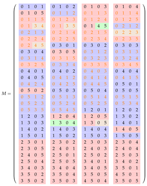
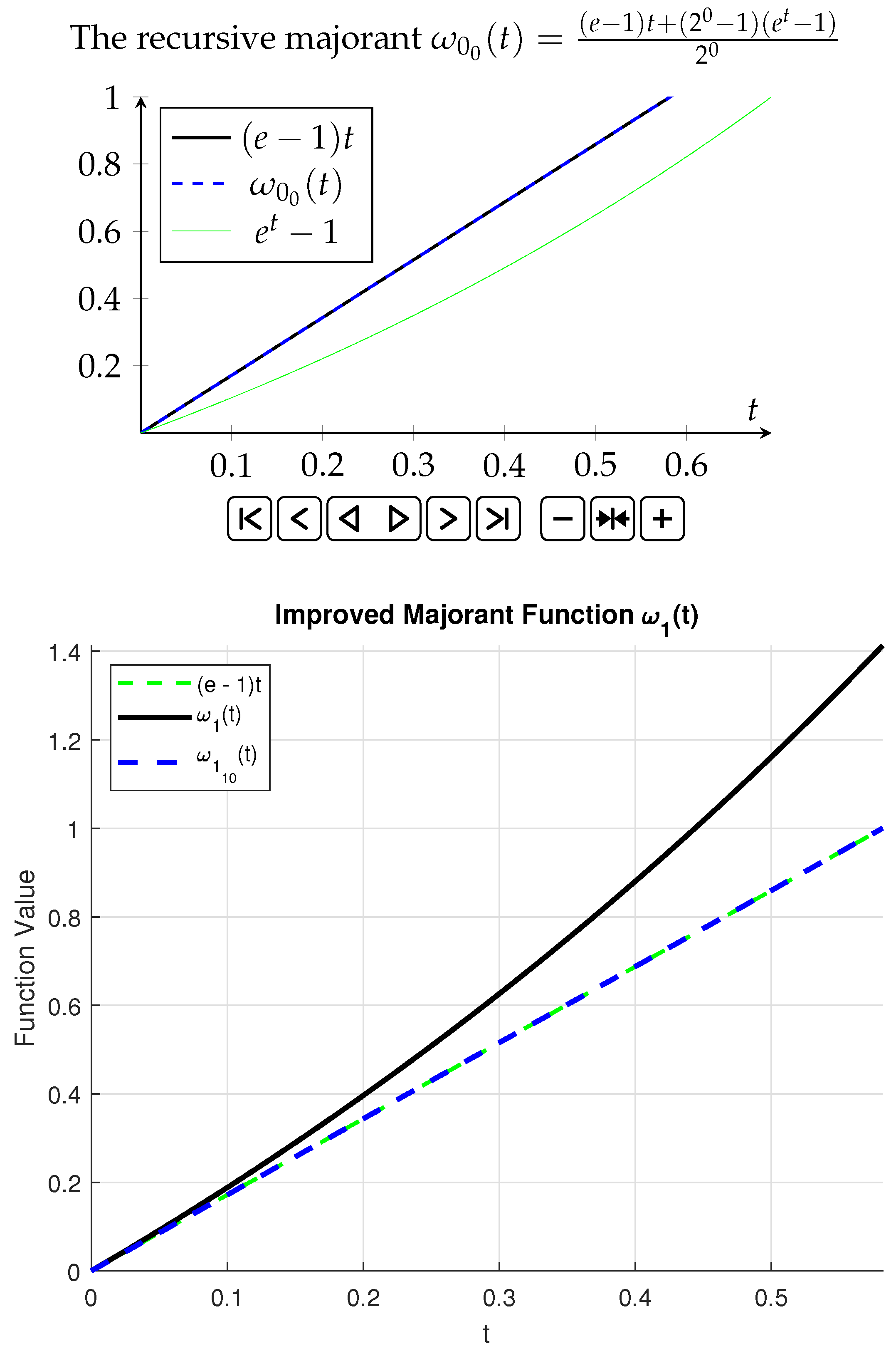

