1. Introduction
Induction motors (IMs) are widely used in various industrial applications due to their robustness, cost-effectiveness, and low maintenance requirements. However, demanding operational conditions often lead to faults in different machine components, with stator faults accounting for approximately 37% of failures and inter-turn short-circuit (ITSC) faults representing 33% of stator failures [
1,
2]. These faults can significantly shorten the motor’s operational lifespan, reduce efficiency, and, in severe cases, lead to complete machine failure.
Conventional fault detection methods often rely on expert knowledge and manual signal analysis, which can be subjective and time-consuming. However, the automatic detection of stator faults has led researchers to develop various techniques based on different types of signals. One such approach involves methods based on the stator’s thermal behavior [
3,
4], which detect thermal anomalies caused by inter-turn faults. While this technique has proven effective in controlled environments, it can be influenced by other heat sources, limiting its applicability in real implementations. In addition, flux-based techniques have also been explored for ITSC detection. These can be categorized into two main approaches: air-gap flux analysis [
5,
6] and stray flux analysis [
7,
8]. While effective, these techniques present specific implementation challenges. Installing internal sensors may be unsafe due to potential mismatches with the machine’s design and construction. Conversely, externally installed sensors are highly susceptible to electromagnetic noise [
9] coming from other machines, increasing the complexity of fault detection. Motor current signature analysis (MCSA) is an alternative to address these limitations. This approach enables fault detection by analyzing fault-related signatures in the motor current signal [
10,
11,
12,
13]. MCSA is widely used due to the ease of installing current sensors, which are less invasive than other techniques.
Fault diagnosis can be formulated as a pattern recognition problem. So, Artificial Intelligence (AI)-based approaches have proven effective and hold great potential for fault detection in rotating machinery applications [
14]. For instance, Oner et al. [
15] introduced a technique leveraging inverter switching statistics and an artificial neural network (ANN) for ITSC fault detection in inverter-fed induction motors. Their approach enables the detection of up to two short-circuited turns (SCTs) under various load conditions, achieving a maximum accuracy of 99.51%. While their method achieves a high accuracy for detecting up to two SCTs, it depends on access to the inverter’s internal signals, which may not be available in typical industrial environments. Another relevant study is that of Gundewar and Kane [
16], which proposes a convolutional neural network (CNN)-based technique for ITSC fault detection using color images derived from stator current phase data. Their method attains accuracy of up to 99.38%, with a minimum detectable fault of two SCTs, under different supply frequency and mechanical load conditions. However, their image transformation approach adds significant preprocessing overhead. Similarly, Nazemi et al. [
17] utilized the fundamental frequency phasor magnitude and the third harmonic, converting them into three-dimensional (3D) images processed by a two-dimensional (2D) CNN. Their method enables the detection of up to three SCTs with a maximum accuracy of 99.98%. Nevertheless, this approach can be sensitive to noise, and the leakage effects can negatively impact it. In addition, Rengifo et al. [
18] proposed extracting diagnostic indicators from the magnitude of the space vector of the stator current signal. These indicators are evaluated using machine learning (ML) techniques, achieving up to 100% accuracy with k-Nearest Neighbor (k-NN) and Support Vector Machine (SVM) classifiers, and detecting incipient faults that affect as little as 4% of a phase. Although they reported high accuracy and detection, their method depends on constructing multiple indicators, which could hinder adaptation to changing operational conditions. Finally, Cardenas-Cornejo et al. [
19] proposed an automatic ITSC detection approach based on geometric and optimization-based techniques applied to three-phase currents combined with ML classifiers. Their method achieves an accuracy of 95.3% across 13 fault classes and can detect damage affecting as little as 1.41% of the stator turns. However, the signal modeling and optimization techniques can be complex and computationally intensive. Despite the high classification accuracy reported by these AI-based approaches, extracting meaningful features from raw signals often involves complex signal processing techniques. These include transformations from the time domain to more complex representations, which can substantially increase the volume and dimensionality of the data to be analyzed. Consequently, more elaborate classification models and processing stages are typically required. This stage can be computationally intensive and may require expert domain knowledge, which poses a significant challenge for real-world deployment and scalability. In this manner, early fault identification remains a challenge due to the incipient nature of these failures.
On the other hand, the rise of CNNs across various domains has enabled the development of highly effective classification systems, particularly in image recognition tasks, including ITSC fault detection. However, since the signals involved in ITSC diagnosis are inherently one-dimensional (1D), transforming them into 2D or even 3D representations introduces additional preprocessing steps. This conversion increases the computational load and complicates the CNN architecture and the overall diagnostic approach. On the contrary, works such as those of Zheng et al. [
20] and She et al. [
21] have used 1D-CNN models to classify 1D signals, avoiding the additional steps described above and reducing the amount of data. The model is based on the Multi-Scale 1D-ResNet, whose structure enables the learning of complex features and achieves a high accuracy rate.
This paper presents a novel technique that employs the derivative of the stator current as a preprocessing stage to enhance the fault-related components associated with ITSC signatures. This signal transformation emphasizes the subtle variations introduced by the fault while preserving the temporal characteristics of the original signal. Unlike previous approaches that require converting one-dimensional signals into 2D or 3D formats, the proposed method operates directly on the 1D signal, significantly reducing preprocessing complexity and computational overhead. A 1D-CNN architecture, inspired by the Multi-Scale 1D-ResNet framework, is then applied for classification. The proposed methodology achieves an accuracy rate from 99.16% up to 100.00% accuracy under different mechanical load conditions, with a minimum detectable fault of three SCTs. Moreover, due to its reduced dimensionality and efficient architecture, the model is well suited for practical deployment in real time or embedded monitoring systems.
The main contributions of this paper are the following: (1) the use of a simple yet effective preprocessing step (the discrete derivative of the stator current) that significantly simplifies the signal processing stage by enhancing fault-related features directly in the time domain; (2) the implementation of a compact convolutional neural network architecture with residual blocks, which improves the learning capacity while maintaining a lightweight model and low computational cost compared to existing approaches; and (3) the detection of only the SCT fault at incipient stages (3 SCTs), regardless of the operative mechanical load.
The structure of this paper is as follows:
Section 2 introduces the main concepts related to stator current signal processing explored in this work, including the derivative-based approach, ITSC fault characteristics, and the overview of the Residual Neural Network (ResNet) architecture.
Section 3 presents the proposed methodology for ITSC fault detection, detailing the design and configuration of the CNN architecture.
Section 4 describes the experimental procedures and presents the obtained results.
Section 5 provides an in-depth discussion and analysis of the obtained results. Finally,
Section 6 offers concluding remarks and outlines directions for future work.
2. Stator Current Signal Processing
The processing of the stator current signal has emerged as a powerful and non-invasive method for diagnosing electrical faults in induction motors, including ITSC. This signal reflects the internal behavior of the machine and can carry valuable fault-related information, making it a convenient choice for condition monitoring.
Among the most established techniques is MCSA, which focuses on detecting characteristic frequency components associated with specific fault types in the stator current spectrum. Stator winding faults can be grouped into turn-to-turn, phase-to-phase, and phase-to-ground faults. This work handles the ITSC fault, a kind of turn-to-turn fault. In this case, ITSC faults cause asymmetry through short-circuited turns that lead to the appearance of sideband frequencies near the fundamental frequency. These frequencies can be expressed as
where
is the fault-related frequency component,
is the supply frequency,
a is a positive integer,
p is the number of pole pairs of the motor,
s is the slip, and
b is an odd index. It is essential to highlight that slips
s directly affect the location of the fault-related frequency component, which consequently causes the fault frequency to shift either closer to or farther from the supply frequency
. This dynamic behavior poses a significant challenge for fault detection, as the fault-related component may become masked by other electrical or mechanical phenomena. Furthermore, the increase in stator current caused by the fault can be easily misinterpreted as a natural consequence of increased mechanical loading, making it difficult to distinguish between healthy and faulty conditions based solely on amplitude variations.
The derivative of the stator current signal can be applied as a preprocessing stage to emphasize the components associated with ITSC faults. This approach enhances the visibility of subtle variations in the signal that are often masked under normal operating conditions. Since the stator current can be modeled as the summation of sinusoidal components, it can be expressed as
where
is the amplitude,
is the angular frequency, and
is the phase of the
i-th sine component. Taking the derivative of this signal with respect to time yields
This operation amplifies the signal components (typically associated with fault-related phenomena) at a rate proportional to their angular frequency
while preserving the overall structure of the original signal. As a result, the derivative enhances the presence of ITSC-related features, making them more distinguishable in subsequent processing stages.
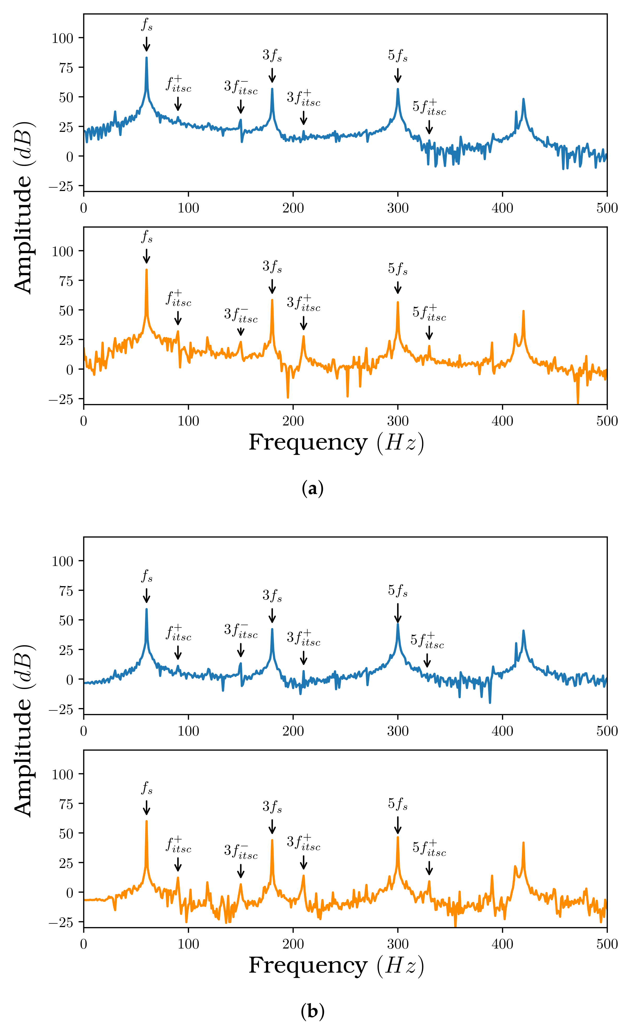
Figure 1 illustrates the effect of applying the derivative on the signal spectrum, emphasizing the enhancement of the
component. Note how the amplitudes of
are amplified in the derivative.
However, a well-known drawback of differentiation is its tendency to amplify high-frequency noise along with the fault-related components, potentially complicating the classification task. The proposed method employs a CNN capable of directly learning robust, noise-tolerant features from the derivative signal to address this challenge. The CNN architecture acts as a powerful filter, effectively distinguishing between relevant fault signatures and unwanted noise, thus improving the overall reliability and accuracy of the detection system.
2.1. ResNet Overview
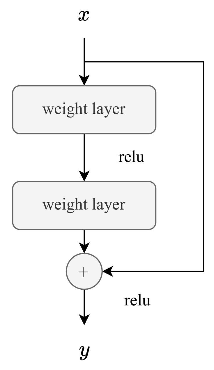
The ResNet architecture was first introduced by He et al. in 2015 [
22], and it marked a breakthrough in deep learning by enabling the training of very deep architectures without suffering from the vanishing gradient problem. The key innovation behind ResNet is the use of identity shortcut connections, which allow the network to learn residual functions, i.e., the difference between the input and output of a layer, instead of learning complete transformations (see
Figure 2). This seemingly simple idea profoundly impacted deep neural networks’ training stability and performance, leading to state-of-the-art results in various computer vision benchmarks such as ImageNet [
23].
While initially developed for image classification using 2D convolutions, the residual learning concept has since been successfully adapted to 1D data, including time-series signals and biomedical waveforms [
24,
25]. Mathematically, it is expressed as follows:
where
represents the residual mapping (e.g., a stack of Conv-ReLU-BN layers). Furthermore, the residual architecture contributes to the method’s robustness by reducing the impact of noise (typically amplified during the derivative operation), thus improving the network’s ability to detect subtle ITSC faults under varying mechanical loads.
This CNN architecture comprises different key layers, each contributing uniquely to the network’s learning capacity and generalization performance. These layers are introduced below.
2.1.1. 1D Convolutional Layer
This convolutional layer is a feature extractor that slides a set of learnable filters (kernels) across the input signal along the time axis. For a given 1D input
, where
N is the number of samples, the output feature map
corresponding to the filter
k is computed as
where
K is the kernel size;
, the weights; and
, the bias. This process enables the model to detect local patterns, such as abrupt changes or distortions.
2.1.2. Batch Normalization
Batch normalization normalizes the output of each convolutional layer to have zero mean and unit variance, computed over each mini-batch. This operation improves training stability and convergence speed and is a regularizer, reducing the risk of overfitting. Its mathematical expression for an input
is presented as follows:
where
is the normalization of
,
is the mini-batch mean,
is the mini-batch variance,
is an small value to avoid zero division, and
and
are learning parameters that allow the network to rescale and displace the normalized output as needed.
2.1.3. ReLU Activation Function
The Rectified Linear Unit (ReLU) is a non-linear activation function defined as
where
x represents an input value. ReLU introduces non-linearity into the network, which is crucial for learning complex representations. In the context of 1D signals, the network can focus on significant features (positive activations), suppressing non-informative or noisy regions (negative values are zeroed out). Additionally, ReLU is computationally efficient and helps mitigate the vanishing gradient problem, which can hamper learning in deep networks.
2.1.4. 1D MaxPooling and Average Pooling Layers
These layers perform temporal downsampling by reducing the dimensionality of the feature maps while retaining the most relevant information.
MaxPooling captures the most dominant feature in each window:
where
s is the stride, and
k is the kernel size. Average pooling computes the average value:
Pooling layers improve computational efficiency and enhance translation invariance in time.
2.1.5. Softmax Activation Layer
Used in the output layer for classification, the softmax function transforms raw outputs into normalized class probabilities:
where
. This enables the model to express its confidence in each class, with the highest probability corresponding to the predicted class.
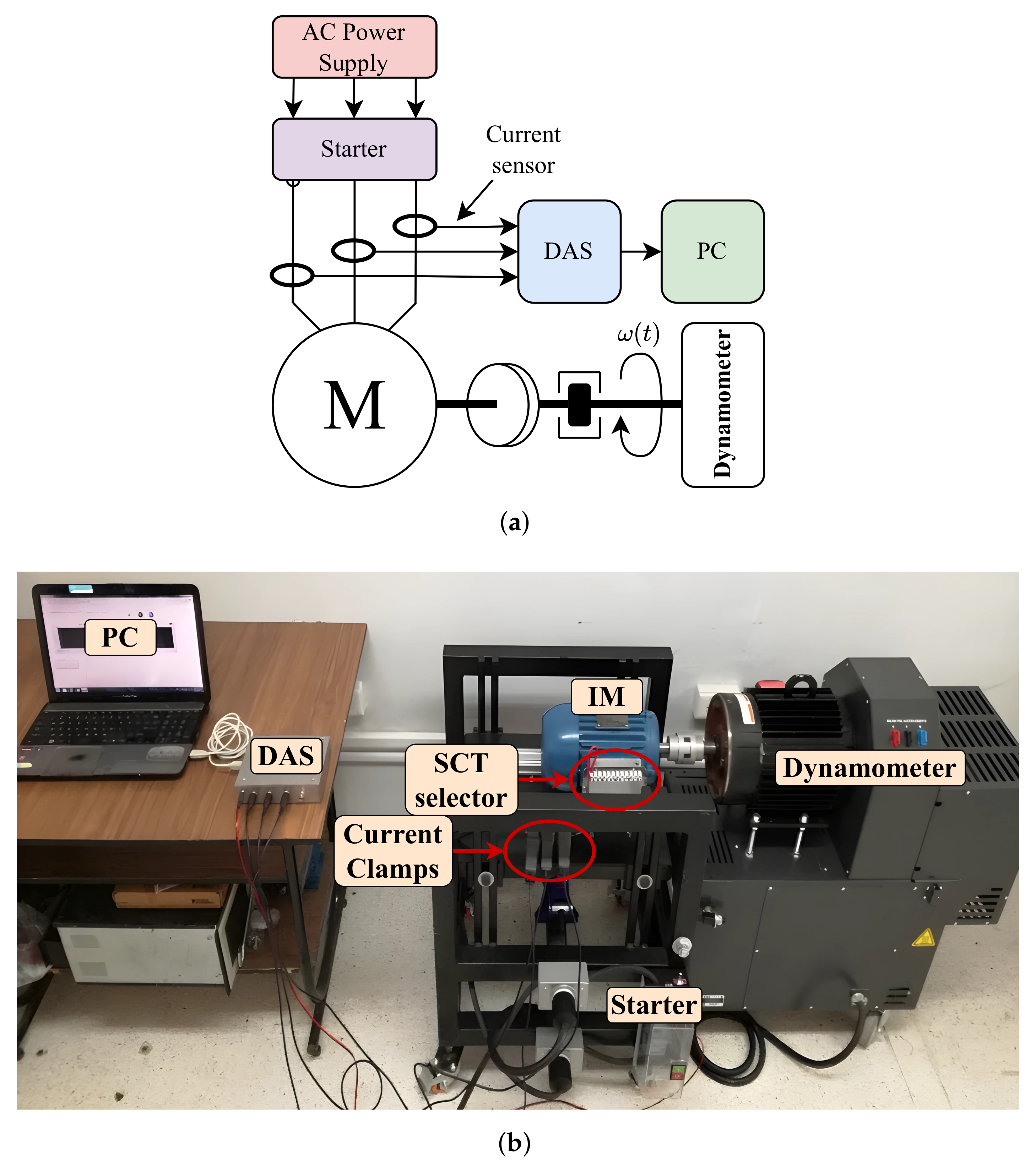
4. Test and Results
The tests were conducted to record the stator current signal under steady-state conditions for 3.5 s per measurement. This duration was selected to prevent severe and irreversible damage to the stator during fault simulations.
To evaluate the proposed method under varying mechanical loads, the dynamometer was configured to apply torques of 0.00, 2.04, 4.09, and 6.13 Nm, corresponding to 0.00%, 33.33%, 66.66%, and 100.00% of the nominal mechanical load, respectively. Combined with the eight different fault conditions (including the healthy case), a total of 32 distinct operating scenarios were generated.
For each scenario, approximately 70 min (in total) of stator current data were acquired at the sampling rate configured in the DAS. The signals were segmented into one-eighth of a second windows to construct the dataset, corresponding to samples per segment in the differentiated signal. This segmentation yielded 18,560 signal segments, forming a comprehensive dataset for training and evaluation purposes.
Figure 7 presents a qualitative comparison between the raw stator current signals (blue) and their corresponding derivatives (orange) for different fault severities, 0, 10, 20, 30, and 40 SCT, considering the configuration and conditions previously described.
Figure 7a corresponds to the no-load condition, while
Figure 7b shows signals under a mechanical load of 4.09 Nm. As the number of short-circuited turns (SCTs) increases, the discrete derivative of the stator current signal reveals sharper and more localized variations in the signal crest compared to the raw current waveform. These variations are especially prominent in amplitude modulation and dynamic frequency components, which tend to intensify with fault severity. The enhanced clarity of these fault-induced features facilitates the extraction of discriminative patterns, improving the classifier’s sensitivity to subtle incipient faults. Consequently, using the current derivative as input to the CNN enhances the network’s ability to detect ITSC faults, as it emphasizes spectral and temporal patterns often obscured in the original time-domain signal.
A standard 80/20 split was applied to divide the dataset into training and testing subsets. The choice of one-eighth-second segments preserved the spectral characteristics associated with fault signatures while maintaining compatibility with the lightweight architecture of the CNN. In addition, five-fold cross-validation was implemented to reduce selection bias and enhance the reliability of the evaluation [
34].
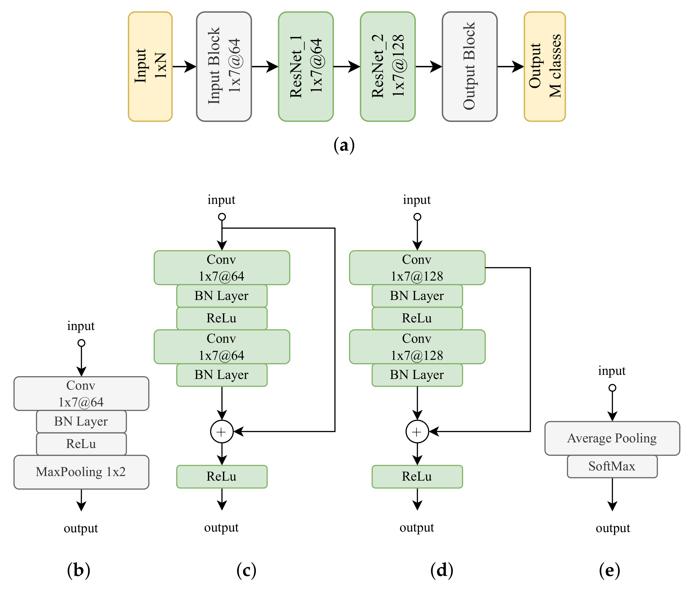
A group of eight classes (
) was defined based on the level of the ITSC fault under study. To ensure that the CNN learned to identify fault-related features independently of mechanical load variations, segments corresponding to the same fault level but different load conditions were grouped into the same class. This approach aims to train the model to focus exclusively on fault characteristics, thereby enabling robust fault detection regardless of variations in load. A summary of the implemented CNN and signal configuration is provided in
Table 5. It is important not to confuse the “Input block” described in
Table 5 with the input layer of the CNN (embedded within the input block; see
Table 1), whose shape is
.
The model was trained for 100 epochs with a batch size of 20. This batch size was selected as a trade-off between training efficiency, memory usage, and execution time. The AdaMax optimizer (
https://keras.io/api/optimizers/adamax/, accessed on 1 June 2025) was employed due to its robustness against noisy gradients, which may arise from the differentiated signal. The results obtained from five-fold cross-validation are presented in
Table 6.
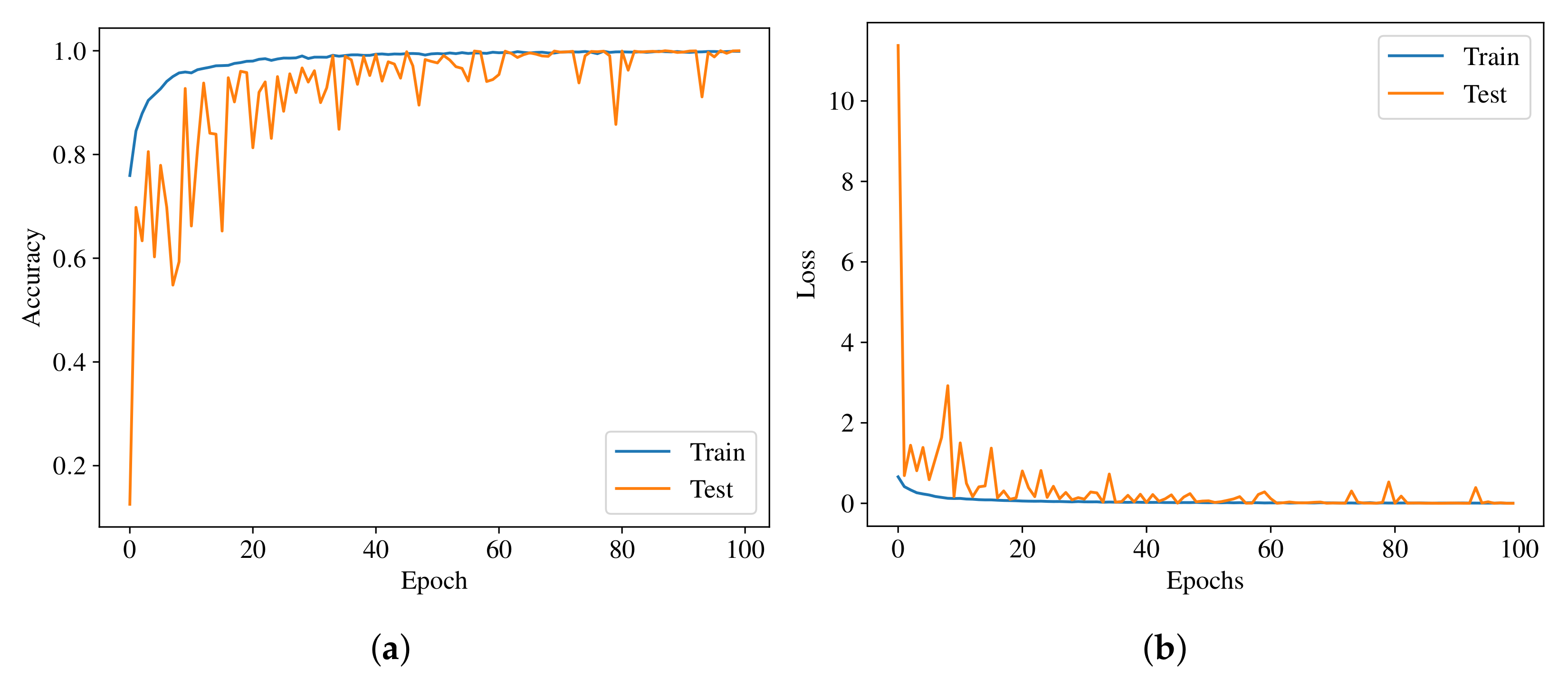
The five-fold cross-validation demonstrates that the proposed model consistently achieves high classification accuracy, with test accuracies ranging from 99.16% to 100%. The corresponding training and test losses remain low, indicating effective learning without signs of overfitting. Notably, the fifth fold yielded a perfect classification accuracy of 100%, further highlighting the robustness of the proposed approach.
Figure 8 illustrates the training process in terms of accuracy and loss over 100 epochs. The training curves show rapid convergence, with accuracy stabilizing around epoch 70, and minimal divergence between training and testing performance, confirming the generalization capability of the CNN.
To provide a clearer picture of the classifier’s performance, confusion matrices for the worst and best cross-validation folds are presented in
Figure 9. In both cases, the confusion matrices exhibit strong diagonal dominance, confirming the model’s ability to accurately identify all eight ITSC fault classes. In the worst-performing scenario (
Figure 9a), a total of 31 signals were misclassified. Specifically, 2 healthy signals under no mechanical load (0.00 Nm) were incorrectly classified as having three SCTs; 1 instance of a five-SCT fault at 2.04 Nm was classified as three SCTs; 18 signals with a three-SCT fault at 4.09 Nm were misclassified as five SCTs; and 10 signals of three SCTs at 6.13 Nm were also incorrectly identified as five SCTs. Among these, the most challenging condition in this fold corresponds to the 4.09 Nm mechanical load, for which the classification accuracy for three SCT faults dropped to 84.48% (98 correctly classified out of 116 signals). However, the few misclassifications in the worst-case scenario are minor and primarily occur between adjacent fault levels, which is expected in real-world fault detection scenarios due to the similarity in signal characteristics, and are associated with the most minor detected fault. These results collectively demonstrate the model’s robustness and its suitability for accurately detecting ITSC faults, regardless of mechanical load variations.
In addition, to further evaluate the performance of the proposed methodology, four testing scenarios were developed to compare the proposed approach with the Multi-Scale 1D-ResNet. Scenario A involves classifying centered and normalized time-series data without applying the derivative, using a segment length of
, as recommended in the Multi-Scale 1D-ResNet. Scenario B incorporates the proposed preprocessing, including the application of the derivative, but also uses
. Scenario C uses the same preprocessing as Scenario A but increases the segment length to
. Finally, Scenario D corresponds to the complete configuration proposed in this work. The results of these scenarios are summarized in
Table 7. The results demonstrate that the proposed preprocessing stage, based on the discrete derivative of the stator current, effectively enhances the spectral signatures associated with ITSC faults. As illustrated in
Figure 7, this processing generates more pronounced and distinguishable patterns than raw signals, particularly as fault severity and mechanical load increase. These clearer spectral features facilitate early-stage fault detection and improve the CNN classifier’s ability to distinguish between fault levels accurately.
The experiments were implemented in Python 3.10 using TensorFlow 2.10 and the Keras 2.10 library. The computational tests were conducted on a laptop model G15 5511 from Dell equipped with an Intel Core i5-11260H @ 2.60 GHz processor, 16 GB of RAM, and an GPU model GeForce RTX 3050 from NVIDIA with 4 GB of dedicated memory. GPU acceleration was enabled following the official setup guidelines provided by the TensorFlow web page [
35].
5. Discussion
Most existing works on ITSC fault detection in induction motors rely on 2D or 3D CNN architectures, which require complex preprocessing and higher computational resources. In contrast, this study proposes a lightweight 1D-CNN model tailored for time-series signals, significantly reducing complexity while maintaining competitive accuracy. The architecture facilitates fast training and is suitable for deployment on non-specialized hardware, making it more practical for real-world applications. Furthermore, the proposed model outperforms or matches the performance of a larger model, the Multi-Scale 1D-ResNet, which inspired this approach.
The results presented in
Table 6 and
Table 7 and
Figure 8 demonstrate the effectiveness of the proposed method for detecting ITSC faults under various mechanical load conditions. The CNN-based model achieved classification accuracies exceeding 99.16% across all five folds of the cross-validation, confirming both its reliability and generalization capacity.
A key element in this performance is the use of differentiated current signals, which enhances fault-related features by emphasizing sharper transitions. Although differentiation may introduce additional noise into the signal, this issue was effectively addressed by employing the AdaMax optimizer. As a robust variant of the Adam algorithm, AdaMax proved remarkably resilient to noisy gradients, contributing to stable and smooth convergence during training.
Another necessary strength of the proposed approach lies in its sensitivity to low-severity faults. The model successfully identified cases with as few as three SCTs, demonstrating its potential for early fault detection. This capability is essential for predictive maintenance applications, where timely intervention can significantly reduce the likelihood of severe motor damage or costly downtime.
Furthermore, the model was designed to generalize across varying mechanical load conditions. By grouping data from different load levels into single classes based on fault severity, the CNN was encouraged to learn features that are strictly fault-related rather than load-dependent. This strategy enhances the model’s robustness and adaptability to real-world industrial environments, where load conditions often fluctuate.
As shown in
Table 7, Scenario D of the proposed approach achieved perfect classification accuracy (100.00%) while requiring only 19.68 min of training, substantially less than the 91.12 min needed for the Multi-Scale 1D-ResNet to reach a slightly lower accuracy (99.95%). Notably, even Scenario B of the proposed model, which used derivative preprocessing with shorter signal segments (
), reached an accuracy of 99.95% in just 16.30 min. These findings emphasize not only the effectiveness but also the relatively low complexity of the proposed solution.
Table 8 provides a comparative overview of recent ITSC fault detection methods. The proposed approach combines the stator current derivative with a lightweight 1D-CNN architecture based on ResNet blocks, achieving an accuracy of 100.00% while detecting faults with as few as three short-circuited turns under four different mechanical load conditions. In comparison, the method by Gundewar and Kane [
16] reaches 99.38% accuracy for two SCTs using a computationally intensive 3D-CNN and image transformations of phase currents. Similarly, Nazemi et al. [
17] employed 2D-CNNs with harmonic features and digital filtering to detect three SCTs with 99.98% accuracy across a wide range of loads. Other works, such as [
18,
36], relied on classical signal processing techniques that involve more complex preprocessing stages. Also, while innovative in applying quaternion analysis, the method by Cardenas-Cornejo et al. [
37] requires six SCTs to reach 99.00% accuracy in no-load conditions. In contrast, the proposed method achieves similar or superior performance with significantly lower complexity, making it a practical and efficient alternative.
It is important to note that the testing environments were developed under steady-state conditions using three-phase, 2 HP induction motors. Nevertheless, the proposed approach is scalable and can be applied to induction motors of different power ratings. This is supported by Equation (
1), which indicates that the fault signature is directly related to the spectral characteristics of the stator current, rather than the power of the machine. Future research will explore extending this methodology to scenarios involving voltage fluctuations and the detection of ITSC faults in non-induction motor types, aiming to further assess its generalization capabilities. In addition, the nature of the studied problem, combined with the inherent plasticity of the employed ResNet-based architecture, as well as the use of fine-tuning and transfer learning techniques, opens the possibility of extending the proposed approach to continuous learning applications, as addressed by Wang et al. [
38] and Ren et al. [
39]. This adaptability suggests strong potential for detecting other types of stator faults and broader applications in industrial rotating machinery, including diagnosing other failure modes and applications in prognosis or adapting to different industrial environment settings, as Chen et al. introduce in [
40]. However, this will be explored in future works.
6. Conclusions
This work presented a lightweight CNN and robust methodology for detecting ITSC faults in squirrel-cage induction motors. The proposed approach combines a derivative-based preprocessing of stator current signals with a custom-designed CNN architecture, achieving accurate fault classification under various mechanical load conditions.
The model demonstrated strong performance, achieving an accuracy of over 99.16% across five-fold cross-validation. It also proved capable of detecting incipient faults as subtle as three SCTs, which is critical for early intervention in predictive maintenance schemes. The use of differentiated signals highlighted fault-related spectral features, thereby improving CNN training efficiency.
Compared with the well-established Multi-Scale 1D-ResNet architecture, the proposed method achieved comparable or better accuracy with significantly lower training times, up to 4.6 times faster. This efficiency positions the technique as an excellent candidate for real-time deployment in embedded systems or industrial applications with limited computational resources.
Future work will focus on validating the model with real-time data acquisition systems and extending the framework to handle other types of motor faults, such as rotor bar breakage or eccentricity, or continuous learning applications. Furthermore, a detailed investigation will be conducted to assess the effectiveness of the methodology in detecting even more incipient faults (involving fewer than three short-circuited turns) as well as under non-ideal electrical conditions, such as voltage fluctuations or unbalanced supply conditions. These extensions could improve the model’s generalization capabilities and broaden its applicability in real-world industrial environments.


 ,
, 


