Article

MultiGNN: A Graph Neural Network Framework for Inferring Gene Regulatory Networks from Single-Cell Multi-Omics Data

1
School of Information, Beijing Forestry University, Beijing 100083, China
2
Risk Assessment Division 1, China National Center for Food Safety Risk Assessment, Beijing 100022, China
*
Authors to whom correspondence should be addressed.
These authors contributed equally to this work.
Computation 2025, 13(5), 124; https://doi.org/10.3390/computation13050124
Submission received: 12 April 2025 / Revised: 9 May 2025 / Accepted: 14 May 2025 / Published: 19 May 2025
(This article belongs to the Topic Computational Intelligence and Bioinformatics (CIB))

Abstract

:
Gene regulatory networks (GRNs) describe the interactions between transcription factors (TFs) and their target genes, playing a crucial role in understanding gene functions and how cells regulate gene expression under different conditions. Recent advancements in multi-omics technologies have provided new opportunities for more comprehensive GRN inference. Among these data types, gene expression and chromatin accessibility are particularly important, as they are key to distinguishing between direct and indirect regulatory relationships. However, existing methods primarily rely on gene expression data while neglecting biological information such as chromatin accessibility, leading to an increased occurrence of false positives in the inference results. To address the limitations of existing approaches, we propose MultiGNN, a supervised framework based on graph neural networks (GNNs). Unlike conventional GRN inference methods, MultiGNN leverages features extracted from both gene expression and chromatin accessibility data to predict regulatory interactions between genes. Experimental results demonstrate that MultiGNN consistently outperforms other methods across seven datasets. Additionally, ablation studies validate the effectiveness of our multi-omics feature integration strategy, offering a new direction for more accurate GRN inference.

1. Introduction

Gene regulatory networks (GRNs) represent the interactions between the transcription factors (TFs) that regulate the expression levels of a genome and the target genes they control [1]. A comprehensive understanding of GRNs is fundamental to explaining how genes function and how cells regulate gene expression under various conditions [2]. Inferring GRNs remains a significant challenge in biology.
Gene regulation is complex and multi-layered, involving factors such as transcription and translation, all of which can affect gene expression. Consequently, inferring regulatory relationships between genes using transcriptomics data alone is highly challenging [3,4,5]. One major limitation is that transcriptomics data cannot distinguish between direct and indirect regulatory interactions, which inevitably leads to the introduction of false positives into the inferred networks [6,7]. To address this issue, DeepTFni [8] infers gene regulatory relationships using chromatin accessibility data. Chromatin accessibility analysis enables the identification of direct regulatory interactions, as active regulatory elements for TF binding and gene regulations are generally accessible [9]. Experimental results from DeepTFni demonstrate that chromatin accessibility data could also provide regulatory information between genes.
With the development of single-cell technologies, scMulti-omics techniques allow us to observe multimodal data within the same cell, which provides new opportunities to reproduce cell types and gene regulation more comprehensively [10,11]. In the field of cell type inference, several studies have found that analyzing transcriptomics data in conjunction with chromatin accessibility data allows for the discovery of additional cell subtypes [12,13]. In the field of GRN inference, there are already several unsupervised learning methods that use multi-omics data to infer GRNs. scMTNI [14] and SCENIC+ [15] first identify TF binding sites by performing motif analysis [16] in accessible chromatin (ATAC peak) regions to construct initial TF–gene or TF–cis-regulatory element (CRE) relationships. MTLRank [17] computes TF activity scores from ChIP-seq and scATAC-seq data to estimate the regulatory effects between each TF and gene in the cell, and combines TF activity with TF expression to predict RNA velocity [18] using a multi-layer neural network. These studies have all found that using gene expression and chromatin accessibility data for GRN inference can better identify direct and indirect regulatory relationships, reduce false positives and false negatives, and improve accuracy.
However, unsupervised methods are affected by the curse of dimensionality when dealing with a large number of genes. To address this issue, a supervised learning framework, CNNC [19], has been proposed. CNNC learns from prior knowledge and infers GRNs using deep convolutional neural networks. Compared to unsupervised models, supervised models can better capture subtle differences between regulated and non-regulated relationships. In recent years, an increasing number of supervised methods for GRN inference have been proposed [20,21,22]. However, they rely solely on gene expression data, without incorporating additional biological information. This limitation can lead to false positives in GRN inference due to the single modality approach.
To overcome this limitation, we propose a new method for inferring GRNs using multi-omics data, called MultiGNN. MultiGNN is a supervised, graph neural network-based framework. It uses a link prediction approach to directly treat the regulatory relationships between genes as learning objectives. Compared to previous supervised methods, our approach learns the subtle differences between direct and indirect gene regulation from both gene expression and chromatin accessibility data. We conducted experiments comparing MultiGNN with several other GRN inference methods across seven datasets. The experimental results demonstrate that our method significantly outperforms the other methods.

2. Materials and Methods

2.1. Datasets

The study used seven publicly available datasets, which consist of scRNA-ATAC-seq data from different tissues of both human and mouse [23,24,25].
In the field of GRN, there has been a persistent lack of real-world networks for model evaluation. In the GRN inference literature, a common practice is to evaluate the accuracy of a resulting network by comparing its edges to an appropriate database of TFs and their targets. Therefore, We utilized the non-specific ChIP-seq provided by BEELINE [3] and the functional interactions from the STRING [26] database as ground truth networks. Statistical data are shown in Table 1.

2.2. Data Preprocessing

We first preprocessed the raw count matrices for scRNA-seq and scATAC-seq of the dataset. For each count matrix, we denoted rows as features (genes or peak regions) and columns as cells throughout the paper below. Each data matrix was removed if a row or column contained less than 0.1% non-zero values. Data quality control was performed by Seurat V4, including but not limited to total read counts, mitochondrial gene ratios, and blacklist ratios [12]. After quality control, we selected the top 1000 highly variable genes for subsequent analyzes based on gene variance, and the final gene expression matrix and chromatin accessibility matrix were obtained. The gene expression matrix was denoted as X R = { x i j R i = 1,2 , , I ; j = 1,2 , , J , with I genes and J cells. The chromatin accessibility matrix was denoted as X A = { x k j A k = 1,2 , , K ; j = 1,2 , , J , which has K peak regions in J cells.
To apply the chromatin accessibility data to GRNs inference, we used the method described in MAESTRO [27] to calculate the peak region in X A as the regulatory potential of the corresponding gene. Specifically, based on the distance between peak k and gene i in the genome, the regulatory potential weight of peak k for gene i is calculated as w i k .
w i k = 0 , d i k > 150   kb or peak k located in any nearby genes 1 L e n g t h e x o n , peak k located at the   exon regions of the gene i   2 d i k d 0 , otherwise ,
where d i k denotes the distance from the center of peak k to the transcriptional starting site of gene i , and d 0 is the half-decay of that distance (set to 10 kb). The regulatory potential w i k of peak k for gene i is usually calculated as 2 d i k d 0 . If d i k > 150   k b , w i k should be less than 0.0005, and in order to save computational time, we set it to 0. In MAESTRO, to better fit the gene expression model, if peak k is located in the exon region of the gene, w i k should be 1 according to the formula. But since reads tend to be located in longer exons than shorter exons, to normalize the likelihood of background reads, the total exon reads were normalized by the total exon length of each gene exon. The peak k regulatory potential of gene i in cell j can then be calculated as:
r i k | j = w i k × x k j A  
Finally, the scATAC-seq matrix X A is transformed into the gene regulatory potential matrix X P by summing the regulatory potential scores of peaks regulating the same gene:
x i j P = k r i k | j  

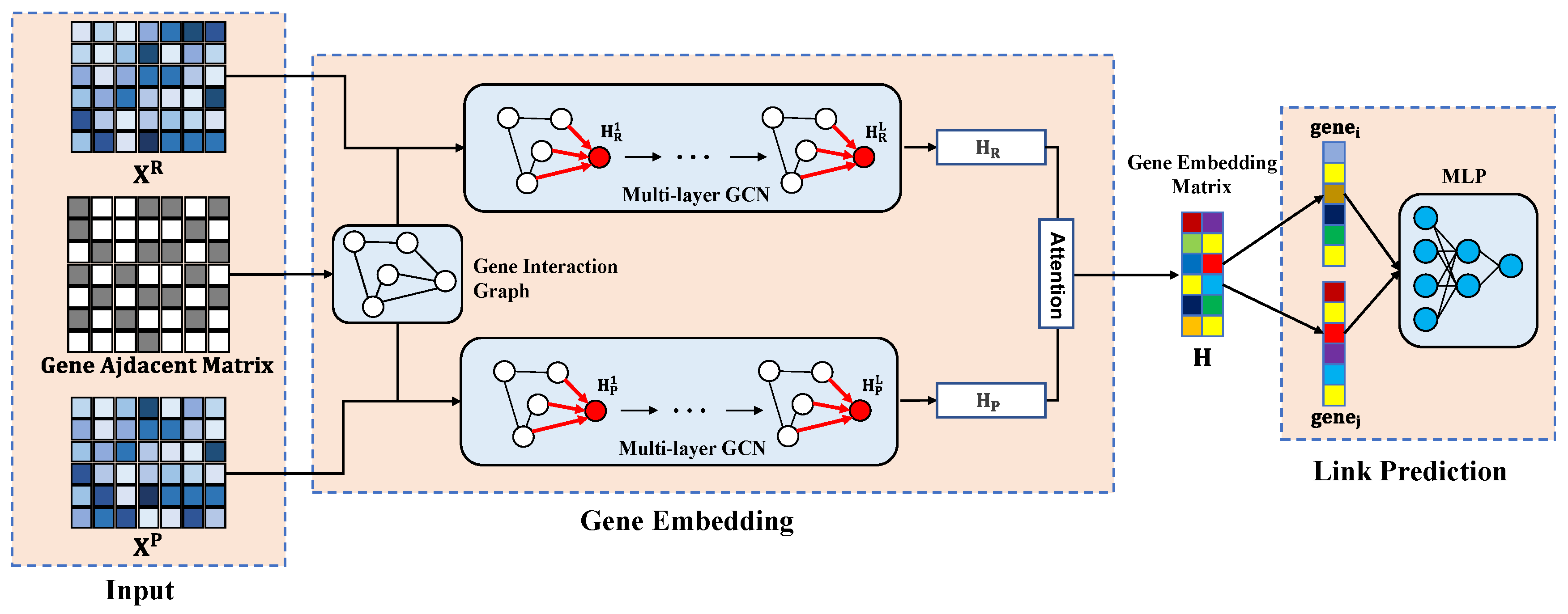
2.3. The MultiGNN Framework

Link prediction is a method for inferring the presence of new or hidden links in a network by using existing network information and node properties. In this area, graph neural networks (GNNs) have made significant progress in recent years [28,29,30]. In the field of GRN inference, there are also a growing number of studies using graph neural network-based techniques [31,32,33]. The results of these studies show that graph neural network-based techniques can better capture the dependencies between genes.
In GRNs, nodes denote TFs or genes, and edges between nodes denote regulatory relationships, which are directed, pointing from TFs to target genes [3]. We denote the priori GRNs by G = V , E , X R , X P , where V = v 1 , v 2 , , v N denotes the set of N nodes, E = { e i j v i   V v j V denotes the set of M edges, X R and X P are the gene expression matrix and the gene regulatory potential matrix, respectively. In gene regulatory network inference, the prior GRNs is typically an incomplete known gene regulatory network. The model treats GRNs inference as a link prediction problem by projecting the gene expression matrix, the gene regulatory potential matrix, and the knowledge-based interaction matrix into a low-dimensional space. Then, by optimizing the low-dimensional space, we learn the features of genes in both the expression matrix and the regulatory potential matrix. These features are used to predict unknown regulatory relationships between genes.
Based on the above idea, we designed the MultiGNN framework as shown in Figure 1. MultiGNN takes G as input and learns the node’s representation matrix H R N × D using a GCN-based graph encoder, where D denotes the dimensionality of the node’s representation. Subsequently, H is taken as input and the score of whether links exist between nodes is predicted by a multilayer perceptron (MLP). Finally, the prediction loss is calculated by accumulating the score for the probability of existence of links.
The matrix H is derived from two pathways; specifically, one pathway uses a graph encoder based on the gene expression matrix X R , while the other uses a graph encoder based on the gene regulatory potential matrix X P . These two pathways are similar in structure. We denote the gene expression matrix-based graph encoder input as G R = V , E , X R , which uses a multi-layer GCN(MGCN) with an average aggregator to obtain the node’s representation based on the gene expression matrix, and H R i l represents v i th node in the l th layer as follow:
H R i l = r e l u A H l 1 W l 1 , ,
where W l 1 denotes the l th layer weight matrix of MGCN, A denotes the adjacency matrix of the graph. X R serves as the value of the initial H R i 0 . Through the above steps, we can finally obtain the node representation matrix H R .
The input to the graph encoder based on gene regulatory potential is denote as G R = V , E , X P , and the node representation H P is obtained using the same method as described above. In order to fuse H R and H P , we use self-attention to learn their relative importance, α R , α P , as follows:
α R , α P = Attention H R , H P ,
where α R , α P R N × 1 . Specifically, We first apply a nonlinear transformation, and then use a shared attention matrix Q R 1 × D to learn its attention scores ω R R N × 1 , as follows:
ω R = tanh H R W P + B Q P ,
where W P R D × D and B R N × D represent the weight and bias matrices, respectively. Using this method, we can also obtain ω P R N × 1 for H P . We normalize ω R using the s o f t m a x formula to obtain α R :
α R = softmax ω R = exp ω R exp ω R + exp ω P
Similarly, α P = s o f t m a x ω P . Let α R = d i a g α R R N × N and α P = d i a g α P R N × N , the final node representation H is obtained by merging H R and H P :
H = α R H R + α P H P
Subsequently, we connect the representations of the two nodes, H i and H j , and input them into the MLP to obtain the score s i j for the existence probability of a link between the two nodes:
s i j = sigmoid W 2 · r e l u W 1 ·   H i ; H j + b 1 + b 2
We use s i j to denote the output of the model’s prediction for the two nodes’ link. In order to optimize the model parameters, we can minimize the binary cross-entropy (BCE) loss:
B C E = 1 M m = 1 M   y m log m o d e l x + 1 y m log 1 m o d e l x   ,
where m denotes the m th TF–gene pair and y m denotes the label of the m th TF–gene pair.

2.4. Experimental Setting and Hyperparameter Optimization

For each real network, we use 4/5 of the set of positive labels as the training set and 1/5 of the positive labels as the test set. Due to the high imbalance of the dataset (as in Table 1), we randomly sampled negative samples in the unobserved links. The training set was constructed with an equal number of positive and negative samples. For the test set, we employed the following sampling strategy to simulate real-world sparse regulatory networks:
N p o s i t i v e N p o s i t i v e + N n e g a t i v e = | E | 1 2 N T F × N g e n e  
where | E | represents the number of edges in the regulatory network of the dataset, N T F and N g e n e denote the number of transcription factors (TFs) and genes, respectively. N p o s i t i v e and N n e g a t i v e represent the number of positive and negative samples in the test set. This widely adopted approach aims to evaluate model performance under biologically realistic conditions where interaction networks are extremely sparse.
In the training set, we performed hyperparameter tuning based on a five-fold cross-validation method. Specifically, the training set was equally divided into five subsets, with one subset iteratively held out as the validation set while the others were used for training. After hyperparameter optimization (experimental results can be found in Figure S1 and Table S1), the number of layers in MGCN was set to 2, with hidden layer sizes of 512 and 128, respectively, while the MLP’s hidden layer size was 256. The training epoch of the model was set to 200, and an exponentially decaying learning rate was used, with an initial rate of 0.001 and a decay of 80% every 20 training epochs.
The baseline methods included in this paper are:
  • GNNLink [33]: uses MGCN to predict potential gene dependencies from scRNA-seq data and gene network topologies.
  • GENELink [31]: proposes a graph attention network approach to infer potential GRNs.
  • GNE [20]: predicts gene relationships by learning transcriptomics data and genomics network topology via MLP.
  • CNNC [19]: predicts GRNs using deep convolutional neural networks.
  • STGRNS [34]: a supervised learning method based on Transformer architecture.
  • GENIE3 [35]: an unsupervised learning method based on random forests that constructs GRNs using regression coefficient weights.
For the methods mentioned above, we adopted the data processing approaches and parameters specified in their respective original publications for model training. Notably, GENIE3 utilized its computationally optimized version, GRNBoost2 [36], to enhance runtime efficiency. For a fair comparison of the models, all models were trained on the same training set and model performance was compared on the same test set. Given the significant imbalance between positive and negative samples in the test set, we adopted both the AUC (area under the ROC curve) and the AUPR (area under the precision–recall curve) metrics to comprehensively evaluate each model’s ability to identify positive samples. The AUC reflects the overall ability of the model to distinguish between positive and negative classes by plotting the true positive rate against the false positive rate at various thresholds. However, in highly imbalanced scenarios, AUC may overestimate model performance due to the overwhelming number of negative samples. In contrast, AUPR focuses on the precision and recall of the positive class, providing a more informative and sensitive evaluation in imbalanced settings. Therefore, the combination of AUC and AUPR allows for a more balanced and robust assessment of model performance.

3. Results

3.1. Performance on Benchmark Datasets

To evaluate the performance of the models, we conducted comprehensive benchmark testing of seven established methods on seven datasets (Figure 2 and Figure S2). MultiGNN achieved the best results on nearly all datasets. Among graph-based learning methods, MultiGNN outperformed GENELink by 12% and 14% in AUPRC metrics for TF+500 and TF+1000, respectively, and surpassed GNNLink by 18% and 18%. This demonstrates the value of cross-modal feature fusion. Notably, traditional non-deep learning methods (GENIE3, GRNBoost2) showed limited performance, highlighting the advantages of deep learning in regulatory inference.
For the human_jejunum dataset with STRING as the ground truth network, all three graph-based methods performed exceptionally well. This is likely attributed to the dataset’s superior data quality and network density—it has the highest network density among all datasets (twice that of the second densest dataset). On the human_kidney dataset, which has the second highest network density, and the human_pbmc dataset, which has the third highest, MultiGNN also performed exceptionally well compared to the other two models (GENELink, GNNLink). As the network density decreased, the performance of all models declined to varying extents, especially the AUPRC score, as seen in the results from TFs+500 to TFs+1000. However, even on the TFs+1000 dataset, MultiGNN maintained good performance, achieving the best AUPRC metric across all datasets. This indicates that MultiGNN demonstrates better predictive performance in complex regulatory systems.
MultiGNN also has an advantage in training time (see Table S2). On half of the datasets (12/24), our model achieves the fastest training speed. Moreover, our speed advantage becomes more pronounced as the dataset size increases. On the largest dataset, human_bone, we only need half the time of the second fastest model, GNNLink, to complete the training. The fast training speed of our model on large datasets demonstrates the excellent computational complexity of our model.

3.2. Multi-Omics Data Enhances Prediction Accuracy

To evaluate the contribution of multi-omics data, we conducted an ablation study comparing three configurations: (1) the RNA model using only gene expression data (MultiGNN_RNA_only), (2) the ATAC model using only chromatin accessibility data (MultiGNN_ATAC_only), and (3) the complete multi-omics model based on attention mechanism fusion (MultiGNN).
Experiments were performed on seven datasets. Each model had its hyperparameter tuned on the training set using five-fold cross-validation, and then tested on the test set to obtain the test results. As shown in Figure 3A, the integrated model demonstrated superior performance across all metrics.
While the multi-omics model showed no significant advantage over the RNA-only model in terms of AUROC, a substantial performance gap was observed between multi-omics and single-omics models when measured by AUPRC. Notably, AUPRC serves as a critical metric for assessing model performance on imbalanced datasets, as it directly reflects a model’s capability to identify positive samples. Our experimental findings demonstrate that incorporating multi-omics data can effectively enhance predictive performance on imbalanced datasets.

3.3. Effectiveness of Feature Fusion in MultiGNN

To verify the effectiveness of using the self-attention mechanism for feature fusion in MultiGNN, we compared three feature fusion methods: (1) directly concatenating features from the two omics types and inputting them into a multi-layer perceptron for prediction (MultiGNN_concate), (2) fusing the two omics features using pre-defined static weight coefficients (MultiGNN_add), and (3) performing dynamic feature fusion via the self-attention mechanism (MultiGNN). Each method was optimized with the best hyperparameters obtained from five-fold cross-validation on the training set. The results are shown in Figure 3B.
On most datasets, the static weighted fusion and direct concatenation methods yielded similar performance. However, the self-attention-based dynamic fusion consistently achieved the best results across all seven datasets. This demonstrates that our proposed self-attention feature fusion method outperforms the other two approaches.

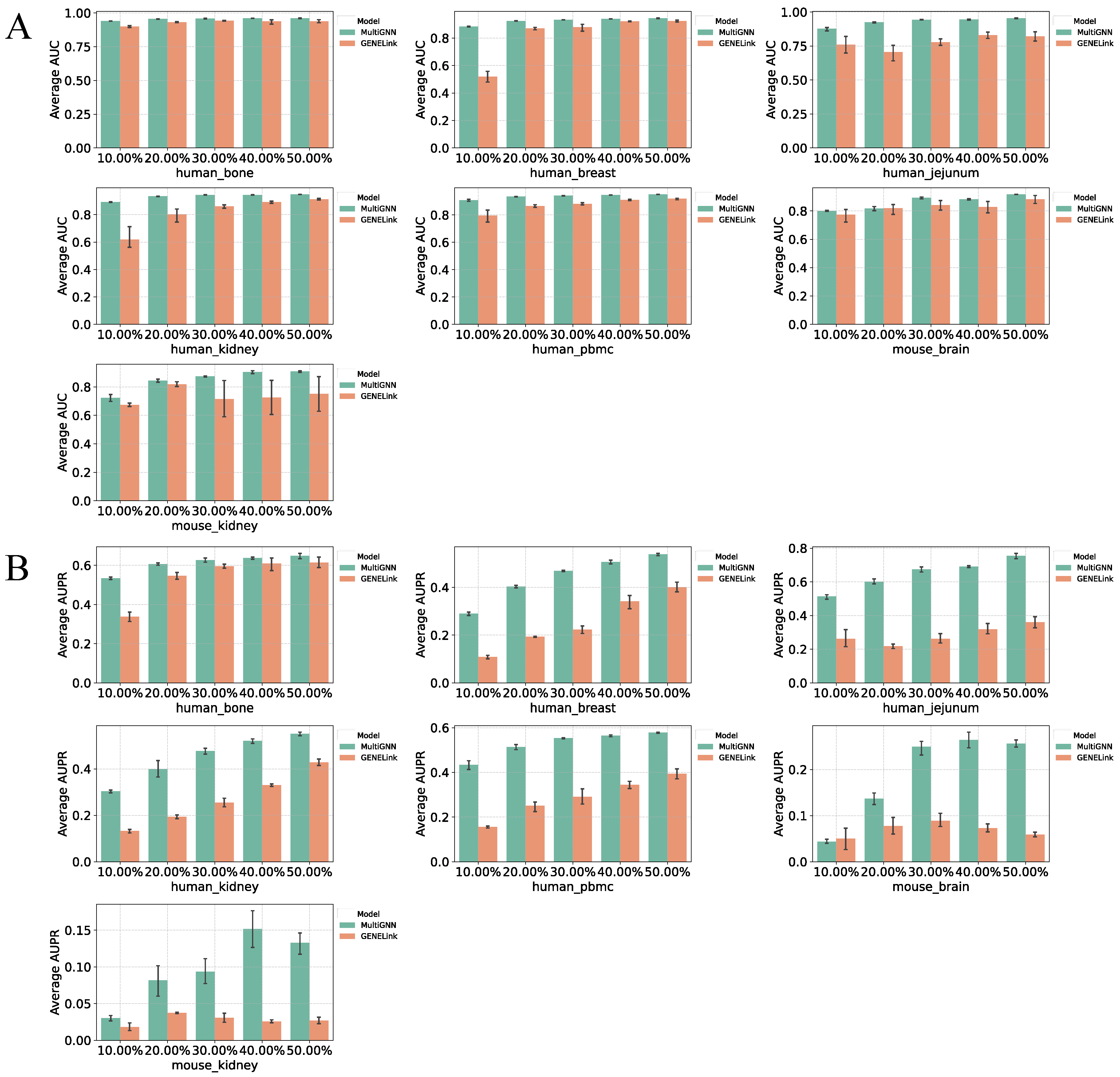
3.4. Robustness of MultiGNN

The MultiGNN is a supervised model, and the size of the training set influences the model’s final performance. Therefore, we investigated the model’s dependence on the dataset size. We trained the model using different proportions of the training set on seven datasets and evaluated its performance on the full test set, as shown in Figure 4. We observed that MultiGNN consistently outperforms GENELink across various dataset sizes.
As the training set size increases, the model accuracy improves, with this effect being particularly evident in the AUPRC metric. On different datasets, the proportion of the dataset required for our model to reach an AUPRC of 0.5 varies. On the human_bone dataset, using only 10% of the data were sufficient to achieve an AUPRC of 0.5, while on the human_breast dataset, more than 50% of the data were needed. This difference is likely related to the absolute number of positive samples in each dataset (the human_bone dataset contains over 10,000 positive samples, while the human_breast dataset only has 2167). From the experimental results, we found that the number of positive samples needed for MultiGNN to achieve an AUPRC of 0.5 is approximately 1000. At this number, GENELink’s AUPRC was only 0.4. These results suggest that MultiGNN has better robustness than GENELink, achieving better performance with smaller datasets.

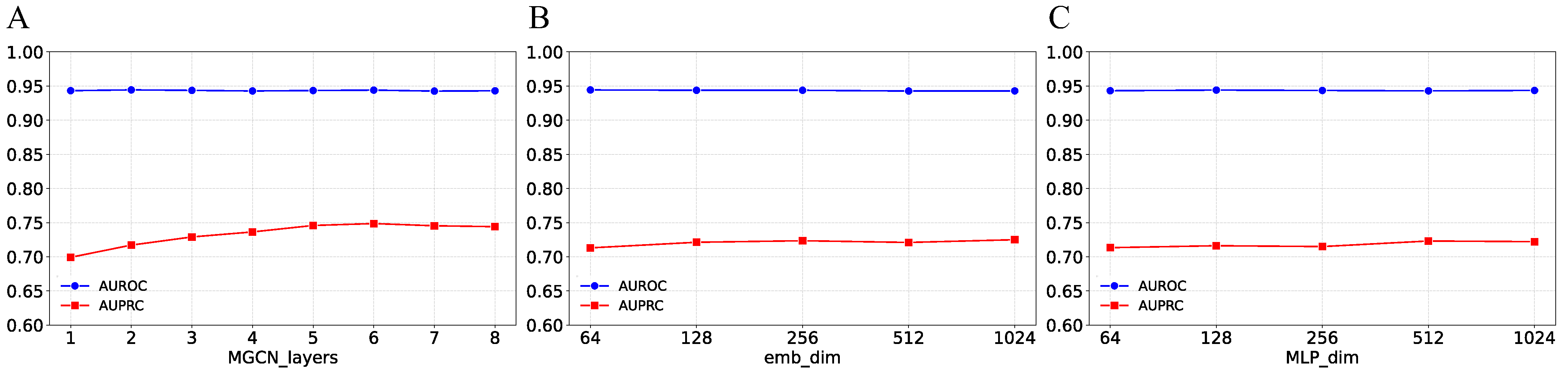
3.5. Parameter Analysis

Unlike the previous section where model parameters were selected for testing, this part focuses on analyzing the sensitivity of MultiGNN to hyperparameters. Therefore, instead of performing five-fold cross-validation on the training set as before, we trained the model on the training set and then observed the impact of hyperparameter choices on the model’s performance on the test set. We analyzed three key parameters in MultiGNN: the number of MGCN layers, the sizes of H R and H P , and the hidden layer size of the MLP. Using the same set of hyperparameter values as in the previous experiments, we varied one parameter at a time while keeping the others fixed. The experimental results are shown in Figure 5. It was observed that the model was not highly sensitive to the sizes of H R and H P or the hidden layer size of the MLP, as changes in these two parameters had a relatively minor effect on the model’s performance. However, the model exhibited greater sensitivity to the number of MGCN layers. We observed that as the number of layers increases, the model showed significant improvement in the AUPRC metric until the number of layers reached five, after which the performance gains began to slow. In contrast, AUROC remained almost unchanged, indicating that increasing the number of MGCN layers enhances the model’s inference capability on imbalanced datasets. This also explains why this phenomenon was not observed during parameter selection on the training set, as the training set consists of an equal number of positive and negative samples.

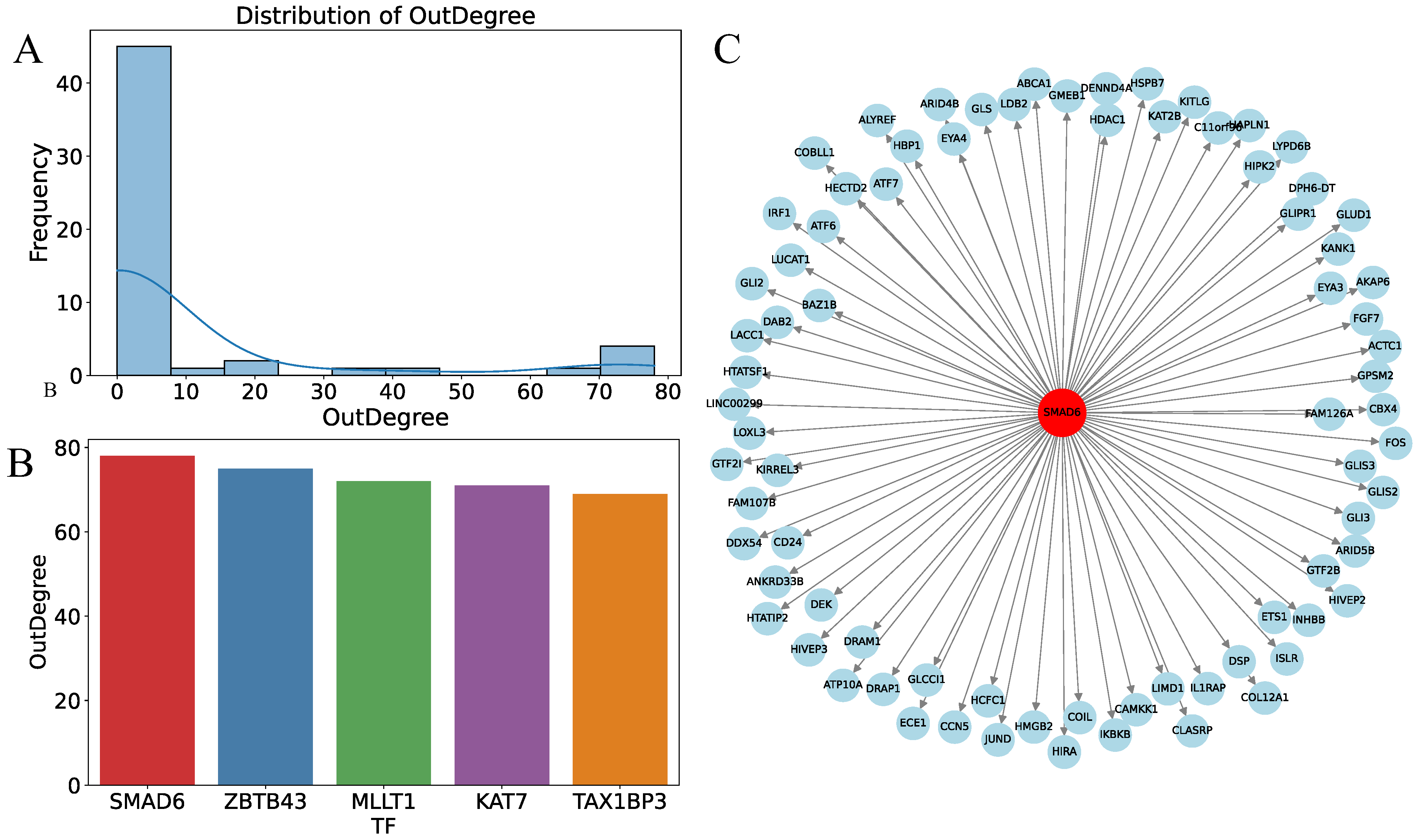
3.6. Prediction of Key Regulatory Factors Using MultiGNN

We performed GRN inference on the human_bone dataset using MultiGNN. The human_bone dataset primarily consists of mesenchymal stem cells (MSCs). MSCs are multipotent stem cells capable of differentiating into osteoblasts, chondrocytes, and adipocytes. During the progression of osteoporosis, the osteogenic differentiation capacity of MSCs is significantly reduced, leading to decreased bone formation. Additionally, MSCs derived from different donors exhibit substantial variability in their osteogenic potential.
From all the predicted unknown regulatory relationships, we selected the top 500 results with the highest prediction scores and analyzed the outdegree of transcription factors (TFs), as shown in Figure 6. The TFs with the highest outdegree were SMAD6, ZBTB43, MLLT1, KAT7, and TAX1BP3. Among them, SMAD6 is an intracellular inhibitor of the bone morphogenetic protein (BMP) signaling pathway, which plays a critical role in osteogenic differentiation. Previous studies have shown that SMAD6 deficiency is associated with various human congenital disorders, including cardiovascular malformations, craniosynostosis, and radioulnar synostosis [37]. The pathogenesis of these diseases is closely related to the abnormal regulation of the BMP signaling pathway. Furthermore, the other transcription factors have also been demonstrated in several studies to play important roles in biological functions and disease mechanisms [38,39,40].

4. Discussion

In recent years, the development of scMulti-omics technology has led to the accumulation of an increasing amount of scMulti-omics data [41]. However, there have been few studies using multi-omics data in the field of supervised GRN inference. The value of incorporating additional biological information has been validated in other fields [15,42,43,44]. Although emerging multi-omics inference models like scMultiomeGRN [45] have been introduced, scMultiomeGRN has not yet been extended to infer TF-gene regulatory relationships. In order to fill the gap of related research, we provide a new approach for inferring GRNs using scMulti-omics data.
We proposed a framework for GRN inference using scMulti-omics data, MultiGNN. This framework learns low-dimensional representations of genes from transcriptomics data and chromatin accessibility data via graph-based encoders and further predicts regulatory relationships among genes. We validated our inference framework on seven scMulti-omics datasets. The results show that MultiGNN outperforms current state-of-the-art models on different metrics. Compared to models using single-omics data, our model delivers more accurate results, even achieving superior performance on smaller datasets.
While multi-omics technologies offer a more comprehensive understanding of gene regulatory mechanisms, they also introduce certain challenges. The first problem we had to solve was how to integrate the scMulti-omics data. To address this problem, we used an approach that computes chromatin accessibility data to form gene regulatory potential, in order to derive gene features from chromatin accessibility data. Our experiments show that such an approach can improve the accuracy of MultiGNN.
Although our method achieved good accuracy, there are still some limitations.
In the ablation experiments on multi-omics and feature fusion, the multi-omics data and feature fusion methods did not have a significant impact on model performance. In these two ablation experiments, they contributed approximately a 5% improvement in AUPRC performance to the model, which appears insufficient to establish the notable advantage of MultiGNN over other models in comparative experiments. We additionally conducted an ablation study on the MLP architecture (Figure S3), revealing that the MLP structure plays a crucial role in gene regulatory network inference. Furthermore, based on our parameter analysis on the test set, the number of layers in MGCN significantly influences the model’s performance on imbalanced datasets. Subsequent experiments could explore using deeper graph convolutional layers for feature extraction.
Another important consideration in our study was the construction of training and test datasets. We adopted a commonly used negative sampling strategy: during training, negative samples were randomly drawn from unobserved gene pairs, and a balanced training set with equal numbers of positive and negative samples was constructed. In contrast, the test set was designed to be imbalanced, reflecting the inherent sparsity of GRNs and aiming to simulate a more realistic inference scenario. However, this strategy may introduce label noise and bias. Specifically, unobserved gene pairs do not necessarily imply the absence of regulatory interactions. In practice, some unconfirmed or yet-to-be-discovered regulatory relationships may be incorrectly labeled as negatives, resulting in false negatives. This mislabeling could adversely affect model training and evaluation. Future work may address this issue by incorporating soft labels [46,47], assigning uncertainty measures to unlabeled gene pairs. This could help mitigate the problem of error propagation introduced by hard labeling and improve the robustness of GRN inference.
While our model performed better than others on small datasets, there is still room for improvement in model performance on these smaller datasets. In the future, transfer learning methods, where models trained on large datasets are fine-tuned on smaller datasets, may help achieve better gene regulatory network inference on small datasets.

Supplementary Materials

The following supporting information can be downloaded at: https://www.mdpi.com/article/10.3390/computation13050124/s1, Figure S1: Validation set AUC vs. epoch; Figure S2: Distribution of GRN prediction performance across seven multi-omics datasets; Figure S3: MLP architecture ablation experiments; Table S1: Partial hyperparameter search results; Table S2: Running time statistics of all models. All the Supplementary Materials were submitted together with the manuscript.

Author Contributions

Conceptualization, D.L. and H.C.; methodology, J.W. and Y.W.; software, D.L.; validation, H.C., J.W. and Y.W.; formal analysis, H.C.; investigation, Y.W.; resources, J.W. and Y.W.; data curation, D.L.; writing—original draft preparation, D.L. and H.C.; writing—review and editing, J.W. and Y.W.; visualization, H.C.; supervision, J.W. and Y.W.; project administration, J.W.; funding acquisition, Y.W. All authors have read and agreed to the published version of the manuscript.

Funding

This research was funded by the National Natural Science Foundation of China, Grant Number: 32302241; National Key Research and Development Program of China, grant number: 2024YFF1106705.

Data Availability Statement

The source code of this work can be found at https://github.com/Sennyou/MultiGNN (accessed on 22 July 2024). The human bone dataset was downloaded from NCBI Gene Expression Omnibus under accession number GSE263178 (https://www.ncbi.nlm.nih.gov/geo/query/acc.cgi?acc=GSE255646, accessed on 22 April 2024). The mouse brain single-cell dataset was downloaded from the 10x Genomics website (https://www.10xgenomics.com/datasets/fresh-embryonic-e-18-mouse-brain-5-k-1-standard-2-0-0, accessed on 9 April 2024). The mouse kidney nuclei dataset was downloaded from the 10x Genomics website (https://www.10xgenomics.com/datasets/mouse-kidney-nuclei-isolated-with-chromium-nuclei-isolation-kit-saltyez-protocol-and-10x-complex-tissue-dp-ct-sorted-and-ct-unsorted-1-standard, accessed on 9 April 2024). The human jejunum nuclei dataset was downloaded from the 10x Genomics website (https://www.10xgenomics.com/datasets/human-jejunum-nuclei-isolated-with-chromium-nuclei-isolation-kit-saltyez-protocol-and-10x-complex-tissue-dp-ct-sorted-and-ct-unsorted-1-standard, accessed on 9 April 2024). The human kidney cancer nuclei dataset was downloaded from the 10x Genomics website (https://www.10xgenomics.com/datasets/human-kidney-cancer-nuclei-isolated-with-chromium-nuclei-isolation-kit-saltyez-protocol-and-10x-complex-tissue-dp-ct-sorted-and-ct-unsorted-1-standard, accessed on 9 April 2024). The human breast dataset was downloaded from NCBI Gene Expression Omnibus under accession number GSM7821208 (https://www.ncbi.nlm.nih.gov/geo/query/acc.cgi?acc=GSM7821208, accessed on 22 April 2024).The human PBMC dataset was downloaded from the 10x Genomics website (https://www.10xgenomics.com/datasets/10-k-human-pbm-cs-multiome-v-1-0-chromium-x-1-standard-2-0-0, accessed on 9 April 2024). Retrieve the two ground-truth networks used in this study from BEELINE (https://zenodo.org/records/3701939, accessed on 28 April 2024).

Conflicts of Interest

The authors declare no conflicts of interest.

References

  1. Kim, J.; Choi, M.; Kim, J.R.; Jin, H.; Kim, V.N.; Cho, K.H. The co-regulation mechanism of transcription factors in the human gene regulatory network. Nucleic Acids Res. 2012, 40, 8849–8861. [Google Scholar] [CrossRef] [PubMed]
  2. Karlebach, G.; Shamir, R. Modelling and analysis of gene regulatory networks. Nat. Rev. Mol. Cell Biol. 2008, 9, 770–780. [Google Scholar] [CrossRef]
  3. Pratapa, A.; Jalihal, A.P.; Law, J.N.; Bharadwaj, A.; Murali, T.M. Benchmarking algorithms for gene regulatory network inference from single-cell transcriptomic data. Nat. Methods 2020, 17, 147–154. [Google Scholar] [CrossRef] [PubMed]
  4. Wang, Y.; Lee, H.; Fear, J.M.; Berger, I.; Oliver, B.; Przytycka, T.M. NetREX-CF integrates incomplete transcription factor data with gene expression to reconstruct gene regulatory networks. Commun. Biol. 2022, 5, 1282. [Google Scholar] [CrossRef]
  5. Wang, J.; Chen, Y.; Zou, Q. Inferring gene regulatory network from single-cell transcriptomes with graph autoencoder model. PLoS Genet. 2023, 19, e1010942. [Google Scholar] [CrossRef]
  6. Fiers, M.W.E.J.; Minnoye, L.; Aibar, S.; González-Blas, C.B.; Atak, Z.K.; Aerts, S. Mapping gene regulatory networks from single-cell omics data. Brief. Funct. Genom. 2018, 17, 246–254. [Google Scholar] [CrossRef]
  7. Crow, M.; Paul, A.; Ballouz, S.; Huang, Z.J.; Gillis, J. Exploiting single-cell expression to characterize co-expression replicability. Genome Biol. 2016, 17, 101. [Google Scholar] [CrossRef]
  8. Li, H.; Sun, Y.; Hong, H.; Huang, X.; Tao, H.; Huang, Q.; Wang, L.; Xu, K.; Gan, J.; Chen, H.; et al. Inferring transcription factor regulatory networks from single-cell ATAC-seq data based on graph neural networks. Nat. Mach. Intell. 2022, 4, 389–400. [Google Scholar] [CrossRef]
  9. Grandi, F.C.; Modi, H.; Kampman, L.; Corces, M.R. Chromatin accessibility profiling by ATAC-seq. Nat. Protoc. 2022, 17, 1518–1552. [Google Scholar] [CrossRef]
  10. Kim, D.; Tran, A.; Kim, H.J.; Lin, Y.; Yang, J.Y.H.; Yang, P. Gene regulatory network reconstruction: Harnessing the power of single-cell multi-omic data. NPJ Syst. Biol. Appl. 2023, 9, 51. [Google Scholar] [CrossRef]
  11. Badia-I-Mompel, P.; Wessels, L.; Müller-Dott, S.; Trimbour, R.; Flores, R.O.R.; Argelaguet, R.; Saez-Rodriguez, J. Gene regulatory network inference in the era of single-cell multi-omics. Nat. Rev. Genet. 2023, 24, 739–754. [Google Scholar] [CrossRef]
  12. Ma, A.; Wang, X.; Li, J.; Wang, C.; Xiao, T.; Liu, Y.; Cheng, H.; Wang, J.; Li, Y.; Chang, Y.; et al. Single-cell biological network inference using a heterogeneous graph transformer. Nat. Commun. 2023, 14, 964. [Google Scholar] [CrossRef] [PubMed]
  13. Lin, X.; Tian, T.; Wei, Z.; Hakonarson, H. Clustering of single-cell multi-omics data with a multimodal deep learning method. Nat. Commun. 2022, 13, 7705. [Google Scholar] [CrossRef] [PubMed]
  14. Zhang, S.; Pyne, S.; Pietrzak, S.; Halberg, S.; McCalla, S.G.; Siahpirani, A.F.; Sridharan, R.; Roy, S. Inference of cell type-specific gene regulatory networks on cell lineages from single cell omic datasets. Nat. Commun. 2023, 14, 3064. [Google Scholar] [CrossRef]
  15. González-Blas, C.B.; De Winter, S.; Hulselmans, G.; Hecker, N.; Matetovici, I.; Christiaens, V.; Poovathingal, S.; Wouters, J.; Aibar, S.; Aerts, S. SCENIC+: Single-cell multiomic inference of enhancers and gene regulatory networks. Nat. Methods 2023, 20, 1355–1367. [Google Scholar] [CrossRef]
  16. Bailey, T.L.; Williams, N.; Misleh, C.; Li, W.W. MEME: Discovering and analyzing DNA and protein sequence motifs. Nucleic Acids Res. 2006, 34, W369–W373. [Google Scholar] [CrossRef]
  17. Song, Q.; Ruffalo, M.; Bar-Joseph, Z. Using single cell atlas data to reconstruct regulatory networks. Nucleic Acids Res. 2023, 51, e38. [Google Scholar] [CrossRef]
  18. La Manno, G.; Soldatov, R.; Zeisel, A.; Braun, E.; Hochgerner, H.; Petukhov, V.; Lidschreiber, K.; Kastriti, M.E.; Lönnerberg, P.; Furlan, A.; et al. RNA velocity of single cells. Nature 2018, 560, 494–498. [Google Scholar] [CrossRef]
  19. Yuan, Y.; Bar-Joseph, Z. Deep learning for inferring gene relationships from single-cell expression data. Proc. Natl. Acad. Sci. USA 2019, 116, 27151–27158. [Google Scholar] [CrossRef]
  20. Kc, K.; Li, R.; Cui, F.; Yu, Q.; Haake, A.R. GNE: A deep learning framework for gene network inference by aggregating biological information. BMC Syst. Biol. 2019, 13, 38. [Google Scholar] [CrossRef]
  21. Chen, J.; Cheong, C.; Lan, L.; Zhou, X.; Liu, J.; Lyu, A.; Cheung, W.K.; Zhang, L. DeepDRIM: A deep neural network to reconstruct cell-type-specific gene regulatory network using single-cell RNA-seq data. Brief. Bioinform. 2021, 22, bbab325. [Google Scholar] [CrossRef] [PubMed]
  22. Zhao, M.; He, W.; Tang, J.; Zou, Q.; Guo, F. A hybrid deep learning framework for gene regulatory network inference from single-cell transcriptomic data. Brief. Bioinform. 2022, 23, bbab568. [Google Scholar] [CrossRef]
  23. Binder, M.; Szalat, R.E.; Talluri, S.; Fulciniti, M.; Avet-Loiseau, H.; Parmigiani, G.; Samur, M.K.; Munshi, N.C. Bone marrow stromal cells induce chromatin remodeling in multiple myeloma cells leading to transcriptional changes. Nat. Commun. 2024, 15, 4139. [Google Scholar] [CrossRef]
  24. Bhat-Nakshatri, P.; Gao, H.; Khatpe, A.S.; Adebayo, A.K.; McGuire, P.C.; Erdogan, C.; Chen, D.; Jiang, G.; New, F.; German, R.; et al. Single-nucleus chromatin accessibility and transcriptomic map of breast tissues of women of diverse genetic ancestry. Nat. Med. 2024, 30, 3482–3494. [Google Scholar] [CrossRef]
  25. 10k Human PBMCs, Single Cell Multiome ATAC Gene Expression Demonstration Data by Cell Ranger ARC 1.0.0, 10x Genomics. 2021. Available online: https://www.10xgenomics.com/datasets/10-k-human-pbm-cs-multiome-v-1-0-chromium-x-1-standard-2-0-0 (accessed on 9 April 2024).
  26. Szklarczyk, D.; Kirsch, R.; Koutrouli, M.; Nastou, K.; Mehryary, F.; Hachilif, R.; Gable, A.L.; Fang, T.; Doncheva, N.T.; Pyysalo, S.; et al. The STRING database in 2023, protein-protein association networks and functional enrichment analyses for any sequenced genome of interest. Nucleic Acids Res. 2023, 51, D638–D646. [Google Scholar] [CrossRef]
  27. Wang, C.; Sun, D.; Huang, X.; Wan, C.; Li, Z.; Han, Y.; Qin, Q.; Fan, J.; Qiu, X.; Xie, Y.; et al. Integrative analyses of single-cell transcriptome and regulome using MAESTRO. Genome Biol. 2020, 21, 198. [Google Scholar] [CrossRef]
  28. Mou, L.; Lu, X.; Li, X.; Zhu, X.X. Nonlocal Graph Convolutional Networks for Hyperspectral Image Classification. IEEE Trans. Geosci. Remote Sens. 2020, 58, 8246–8257. [Google Scholar] [CrossRef]
  29. Cui, Z.; Henrickson, K.; Ke, R.; Wang, Y. Traffic Graph Convolutional Recurrent Neural Network: A Deep Learning Framework for Network-Scale Traffic Learning and Forecasting. IEEE Trans. Intell. Transp. Syst. 2020, 21, 4883–4894. [Google Scholar] [CrossRef]
  30. Liu, Y.; Yang, S.; Xu, Y.; Miao, C.; Wu, M.; Zhang, J. Contextualized Graph Attention Network for Recommendation with Item Knowledge Graph. IEEE Trans. Knowl. Data Eng. 2023, 35, 181–195. [Google Scholar] [CrossRef]
  31. Chen, G.; Liu, Z. Graph attention network for link prediction of gene regulations from single-cell RNA-sequencing data. Bioinformatics 2022, 38, 4522–4529. [Google Scholar] [CrossRef]
  32. Yuan, Y.; Bar-Joseph, Z. GCNG: Graph convolutional networks for inferring gene interaction from spatial transcriptomics data. Genome Biol. 2020, 21, 300. [Google Scholar] [CrossRef] [PubMed]
  33. Mao, G.; Pang, Z.; Zuo, K.; Wang, Q.; Pei, X.; Chen, X.; Liu, J. Predicting gene regulatory links from single-cell RNA-seq data using graph neural networks. Brief. Bioinform. 2023, 24, bbad414. [Google Scholar] [CrossRef] [PubMed]
  34. Xu, J.; Zhang, A.; Liu, F.; Zhang, X. STGRNS: An interpretable transformer-based method for inferring gene regulatory networks from single-cell transcriptomic data. Bioinformatics 2023, 39, btad165. [Google Scholar] [CrossRef]
  35. Huynh-Thu, V.A.; Irrthum, A.; Wehenkel, L.; Geurts, P. Inferring regulatory networks from expression data using tree-based methods. PLoS ONE 2010, 5, e12776. [Google Scholar] [CrossRef]
  36. Moerman, T.; Santos, S.A.; González-Blas, C.B.; Simm, J.; Moreau, Y.; Aerts, J.; Aerts, S. GRNBoost2 and Arboreto: Efficient and scalable inference of gene regulatory networks. Bioinformatics 2019, 35, 2159–2161. [Google Scholar] [CrossRef]
  37. Luyckx, I.; Verstraeten, A.; Goumans, M.-J.; Loeys, B. SMAD6-deficiency in human genetic disorders. NPJ Genom. Med. 2022, 7, 68. [Google Scholar] [CrossRef]
  38. Kabra, A.; Bushweller, J. The Intrinsically Disordered Proteins MLLT3 (AF9) and MLLT1 (ENL)—Multimodal Transcriptional Switches With Roles in Normal Hematopoiesis, MLL Fusion Leukemia, and Kidney Cancer. J. Mol. Biol. 2022, 434, 167117. [Google Scholar] [CrossRef]
  39. Wang, W.; Zheng, Y.; Sun, S.; Li, W.; Song, M.; Ji, Q.; Wu, Z.; Liu, Z.; Fan, Y.; Liu, F.; et al. A genome-wide CRISPR-based screen identifies KAT7 as a driver of cellular senescence. Sci. Transl. Med. 2021, 13, eabd2655. [Google Scholar] [CrossRef]
  40. Reinstein, E.; Orvin, K.; Tayeb-Fligelman, E.; Stiebel-Kalish, H.; Tzur, S.; Pimienta, A.L.; Bazak, L.; Bengal, T.; Cohen, L.; Gaton, D.D.; et al. Mutations in TAX1BP3 cause dilated cardiomyopathy with septo-optic dysplasia. Hum. Mutat. 2015, 36, 439–442. [Google Scholar] [CrossRef]
  41. Ogbeide, S.; Giannese, F.; Mincarelli, L.; Macaulay, I.C. Into the multiverse: Advances in single-cell multiomic profiling. Trends Genet. 2022, 38, 831–843. [Google Scholar] [CrossRef]
  42. Pickett, S.J.; Hudson, G.; Greaves, L.C. Single-cell multiomic analyses sheds light on mitochondrial mutational selection. Nat. Genet. 2023, 55, 1083–1085. [Google Scholar] [CrossRef] [PubMed]
  43. Ledru, N.; Wilson, P.C.; Muto, Y.; Yoshimura, Y.; Wu, H.; Li, D.; Asthana, A.; Tullius, S.G.; Waikar, S.S.; Orlando, G.; et al. Predicting proximal tubule failed repair drivers through regularized regression analysis of single cell multiomic sequencing. Nat. Commun. 2024, 15, 1291. [Google Scholar] [CrossRef] [PubMed]
  44. Weng, C.; Gu, A.; Zhang, S.; Lu, L.; Ke, L.; Gao, P.; Liu, X.; Wang, Y.; Hu, P.; Plummer, D.; et al. Single cell multiomic analysis reveals diabetes-associated β-cell heterogeneity driven by HNF1A. Nat. Commun. 2023, 14, 5400. [Google Scholar] [CrossRef]
  45. Xu, J.; Lu, C.; Jin, S.; Meng, Y.; Fu, X.; Zeng, X.; Nussinov, R.; Cheng, F. Deep learning-based cell-specific gene regulatory networks inferred from single-cell multiome data. Nucleic Acids Res. 2025, 53, gkaf138. [Google Scholar] [CrossRef]
  46. Jiang, J.; Ge, W.; Wang, Y.; Cheng, Y.; Xu, Y. Soft-label recover based label-specific features learning. Sci. Rep. 2024, 14, 23099. [Google Scholar] [CrossRef]
  47. Liu, Y.; Wang, Y.; Sowmya, A.; Chen, F. Soft Hough Forest-ERTs: Generalized Hough Transform based object detection from soft-labelled training data. Pattern Recognit. 2016, 60, 145–156. [Google Scholar] [CrossRef]
Figure 1. Overview of MultiGNN framework.
Computation 13 00124 g001
Figure 2. Summary of GRN prediction performance across seven multi-omics datasets. The results for each metric, AUROC (A) and AUPRC (B), are the averages obtained after five runs. A total of seven datasets and two ground truth networks (Non-specific ChIP-seq, STRING) are included. Each multi-omics dataset consists of transcription factors (TFs) and either 500 highly variable genes (left) or 1000 highly variable genes (right).
Computation 13 00124 g002
Figure 3. The ablation experiments of MultiGNN were performed on seven datasets from the non-specific ChIP-seq ground truth network. (A) displays the test results of MultiGNN using multi-omics versus single-omics data. (B) shows the test results with different multi-omics feature fusion approaches.
Computation 13 00124 g003
Figure 4. The robustness tests of MultiGNN were performed on seven datasets from the non-specific ChIP-seq ground truth network. AUROC (A) and AUPRC (B) results from running the MultiGNN and GENELink five times on seven datasets with different proportions of the training set.
Computation 13 00124 g004
Figure 5. Sensitivity analysis of MultiGNN parameters. (A) Analysis of the number of MGCN layers. (B) Analysis of the sizes of H R and H P . (C) Analysis of the hidden layer size in the MLP. The results for each parameter represent the average of five runs across seven datasets.
Computation 13 00124 g005
Figure 6. GRN inference using MultiGNN on the human_bone dataset. (A) Outdegree statistics of TFs in the GRN inference results. (B) The top five TFs with the highest outdegree in the GRN inference results. (C) Predicted regulatory relationships of SMAD6.
Computation 13 00124 g006
Table 1. Statistics of scRNA-ATAC-seq datasets and two ground-truth networks composed of TFs and the top 500 most variable genes. The numbers in parentheses in the table represent corresponding statistics for networks composed of TFs and the top 1000 most variable genes.
DatasetCellsNon-Specific ChIP-SeqSTRING
TFsGenesDensityTFsGenesDensity
humanbone6742717 (722)1217 (1566)0.032 (0.029)792 (796)937 (1113)0.051 (0.045)
breast1446186 (190)447 (693)0.052 (0.043)223 (231)300 (435)0.070 (0.055)
jejunum536857 (59)124 (166)0.134 (0.117)81 (84)87 (105)0.133 (0.116)
kidney13,666175 (176)407 (583)0.060 (0.053)226 (230)277 (344)0.065 (0.057)
pbmc6984186 (196)551 (869)0.055 (0.046)230 (235)375 (562)0.061 (0.051)
mousebrain4362100 (109)137 (167)0.028 (0.025)
kidney12,35572 (81)122 (155)0.036 (0.034)
Disclaimer/Publisher’s Note: The statements, opinions and data contained in all publications are solely those of the individual author(s) and contributor(s) and not of MDPI and/or the editor(s). MDPI and/or the editor(s) disclaim responsibility for any injury to people or property resulting from any ideas, methods, instructions or products referred to in the content.

