1. Introduction
Gene networks in living organisms regulate basic processes and participate in the control of vital functions. They are extensively studied by teams of investigators of various kinds: biologists, chemists, physicists, geneticists, statisticians, and mathematicians. Mathematical models are actively used to study gene networks. Models of gene regulatory networks are diverse. They can be deterministic or stochastic. In deterministic models, the future states of a system are determined by the initial state and external input. Due to the possible chaotic behavior of solutions, this does not make it easier to analyze future states. On the other hand, in real-world systems, the stochastic effects may play an important role. Stochastic models are not always necessary; it depends on the modeled system. Generally, genetic networks possess mechanisms that contribute to their overall stability. Maintaining a balance between complexity and stability is important for properly functioning biological systems. When the switch-like behavior among groups of genes is observed, discrete models (such as Boolean algebra and graph theory-based) may be preferable. The evolution of a network in time can be modeled using ordinary differential equations. Details on this topic are available in review articles [
1,
2,
3,
4,
5].
Our focus is on models formulated as dynamical systems. There are numerous models. Some are mentined in review article [
6]. The difference model is described where the increase in the expression level of gene
i at time
t + Δ
t is dependent on the sum of weighted expression levels of other genes at time t. An artificial neural network (ANN) method is mentioned that is capable of describing the dynamic behavior of genetic regulatory networks (GRNs). An inhibitory model of three ordinary differential equations (sometimes referred to as the “Goodwin Oscillator”) was analyzed in [
7]. Typically, ODE models of gene networks incorporate nonlinearities that are expressed using sigmoidal functions. In [
8], an algorithm for qualitative simulation of gene regulatory networks with steep sigmoidal functions is provided. In [
9], there is a focus on “a mechanistic understanding of the gene regulation underneath”. For this, a single-cell model is studied. The author claims that “resolving gene expression in individual cells can allow subtle behaviors to be detected, and by achieving these feats with thousands to millions of data points per experiment, single-cell approaches promise to properly grasp the complexity of biological systems”. In [
10], GRNs are treated as chemical reaction networks. For this, the ODE apparatus is needed. For example, the kinetics of the
lac operon interpreted as a CRN is described by a system of eleven ODEs. In [
11], “Several commonly used network modeling paradigms are surveyed with emphasis on their practical use in systems biology research”. When speaking about ODEs modeling genetic networks, the authors say that “the central idea is to model the rate of change in each reaction as a set of differential equations. These differential equations are coupled, which means the rate of change in the expression of a gene is affected by the current expression level of other genes. When formulating an ODE model, it is important to choose the right balance between model complexity, identifiability, and interpretability”. It is also noted that “it is usually impractical to model all the physical biomolecular processes in a GRN (such as transcription, translation, translocation, and so on). Many have proposed to model functional relationships among genes instead”.
The concept of neural ODEs that belongs to the field of deep learning and its application for modeling GRNs are discussed in [
12]. The modeling framework based on neural ODEs is proposed and tested in a series of experiments involving realistic GRNs. In [
13] the authors present “an extended model for gene regulatory networks with time delayed negative feedback, which is described by delay differential equations”. In [
14] “the finite volume discretization scheme for partial integro-differential equations (PIDEs) describing the temporal evolution of protein distribution in gene regulatory networks is proposed”. This ODE-based model “allows the application of the theory of nonnegative and compartmental systems for the qualitative analysis of the approximating dynamics”. The goal of article [
15] “is to develop genetic networks with temporal delays, which are crucial for genetic regulation because slow biochemical processes like gene transcription and translation need time to occur”.
System (2) in the article under review has a long history. In 1972, H. Wilson and J. Cowan studied the interaction of two populations of neurons, active and inhibitory [
16]. The qualitative analysis of the phase plane for a two-dimensional system was performed. A simplified system in the form (1) was studied qualitatively and numerically in [
17,
18]. The structure of the phase plane and the behavior of solutions were in focus. The 3D system was considered in several sources providing new results on the possible behavior of solutions. An interesting question of the role of stochasticity in cellular reaction dynamics resulting in the selection of a stable gene expression pattern was investigated in [
19]. Gene regulation with positive and negative feedback in an
n-dimensional model (2) was studied in [
18]. System (2) was treated as “a neural network, where each node represents a particular gene and the wiring between the nodes defines regulatory interactions”.
The second group of related results, focusing on the construction of systems with a block diagonal regulatory matrix W and considering systems in search of chaos, is associated with the work [
20] and the literature therein. In [
21], the 6D example of system (2) was examined.
The third group of problems concerns biomedicine-oriented applications of systems of the form (2). In [
22,
23], system (2) was considered as a model suitable for considering and finding ways of treating leukemia (a kind of blood cancer). In a model, the problem is interpreted as going the system state trajectories to a “wrong” attractor. The ways of redirecting trajectories to a “normal” attractor were discussed in [
24,
25].
The fourth group of problems involves identifying chaotic attractors within system (2). Although numerous chaotic attractors may exist in systems of type (2), their discoveries are rare. References [
26,
27] document the same 3D chaotic attractor. The chaotic attractors in a 3D system of type (2) are discussed in [
28,
29].
The dynamics and evolution of networks can be captured by
n-dimensional ODE-based models. Attracting sets play a crucial role in these models, as they define the configuration of phase spaces and enable important conclusions about trajectories and the properties of the modeled networks. Each network element is represented by a time-dependent value of
xi(
t). The components of the network are connected by certain relations, which are described by the regulatory matrix
W, which is built into the system. The current state of the network is represented by the vector
X(
t) = (
x1(
t),…,
xn(
t)), which contains all the elements of the network. The structure of the proposed system ensures that the system’s trajectories, represented by the vectors
X(
t), are confined within a specific bounded region of the phase space. Consequently, the system can have attractors, which are sets that attract trajectories. Describing attractors in a system of differential equations is crucial for forecasting the network’s future states. Available examples suggest that attractors can take the form of critical points, periodic attractors, and more complex sets emerging from the chaotic behavior of the system’s solutions. Various types of attractors have been discovered in two-dimensional models, three-dimensional models, and higher-dimensional individual systems. The study of attractors is not an easy task, since GRN systems contain many parameters, the number of which increases significantly as the dimensionality of the system increases. In this paper, a four-dimensional (4D for short) model of a gene network containing 28 parameters is studied. The work consists of two parts, in which the 4D model is studied using the approaches previously used by the authors. In the first part, systems are built, which are initially a combination of two 2D systems with known properties. These two 2D systems are made dependent, combining into one 4D system, with the help of special techniques. Initially, two two-dimensional systems with periodic attractors are merged into a four-dimensional system. The same process is then applied to another pair of 2D systems, each possessing a periodic attractor. Next, both pairs are included in a family of 4D systems, depending on the parameter
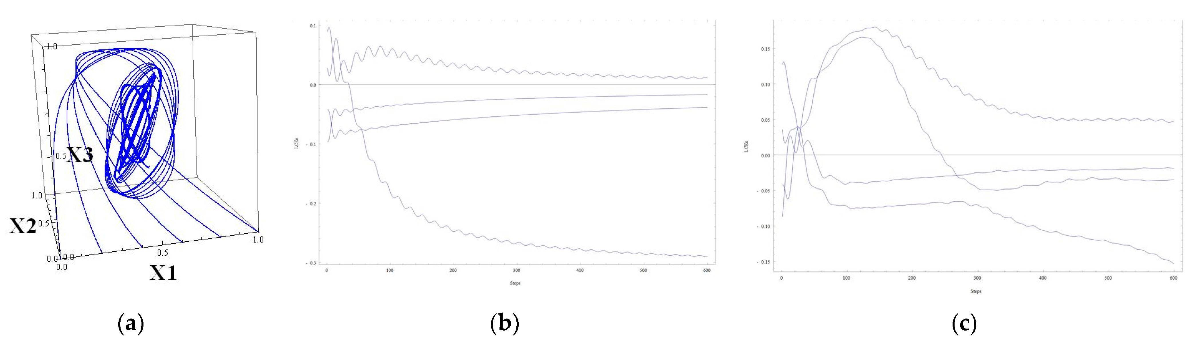
p, which varies in the interval [0, 1]. For
p = 0 we have the first 4D system; for
p = 1 the second one is obtained. Scanning the resulting family of 4D systems by changing the parameter
p, we obtained an attractor, the projection of which on the first three axes is depicted in
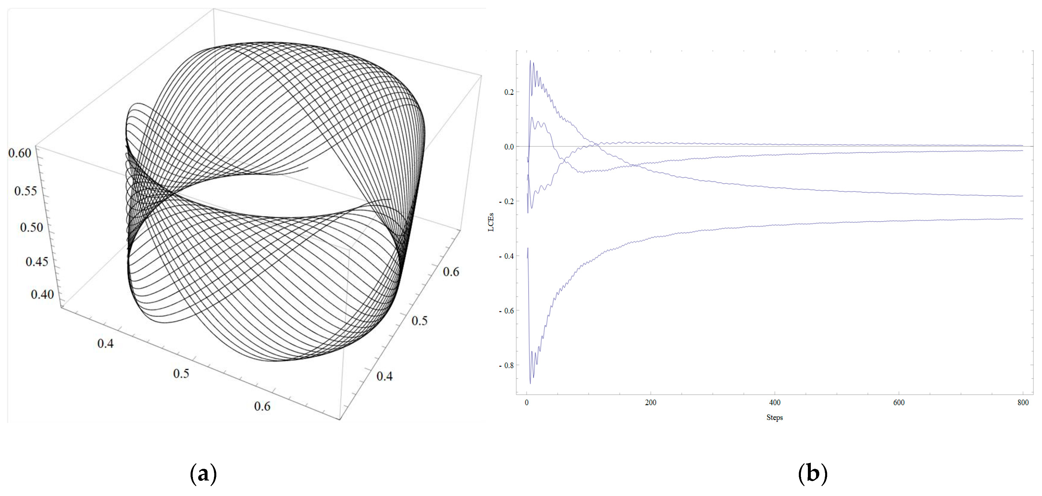
Figure 1. In the next example, the two 2D systems are similarly combined into one 4D system. The first 2D system has an attractor in the form of a limit cycle with clockwise rotation. The second 2D system has an attractor as a limit cycle with counterclockwise rotation. The resulting 4D system is perturbed by adding nonzero elements to the regulatory matrix. An attractor appears in the resulting 4D system. The sensitive dependence of solutions on the initial data is observed by constructing the Lyapunov exponents [
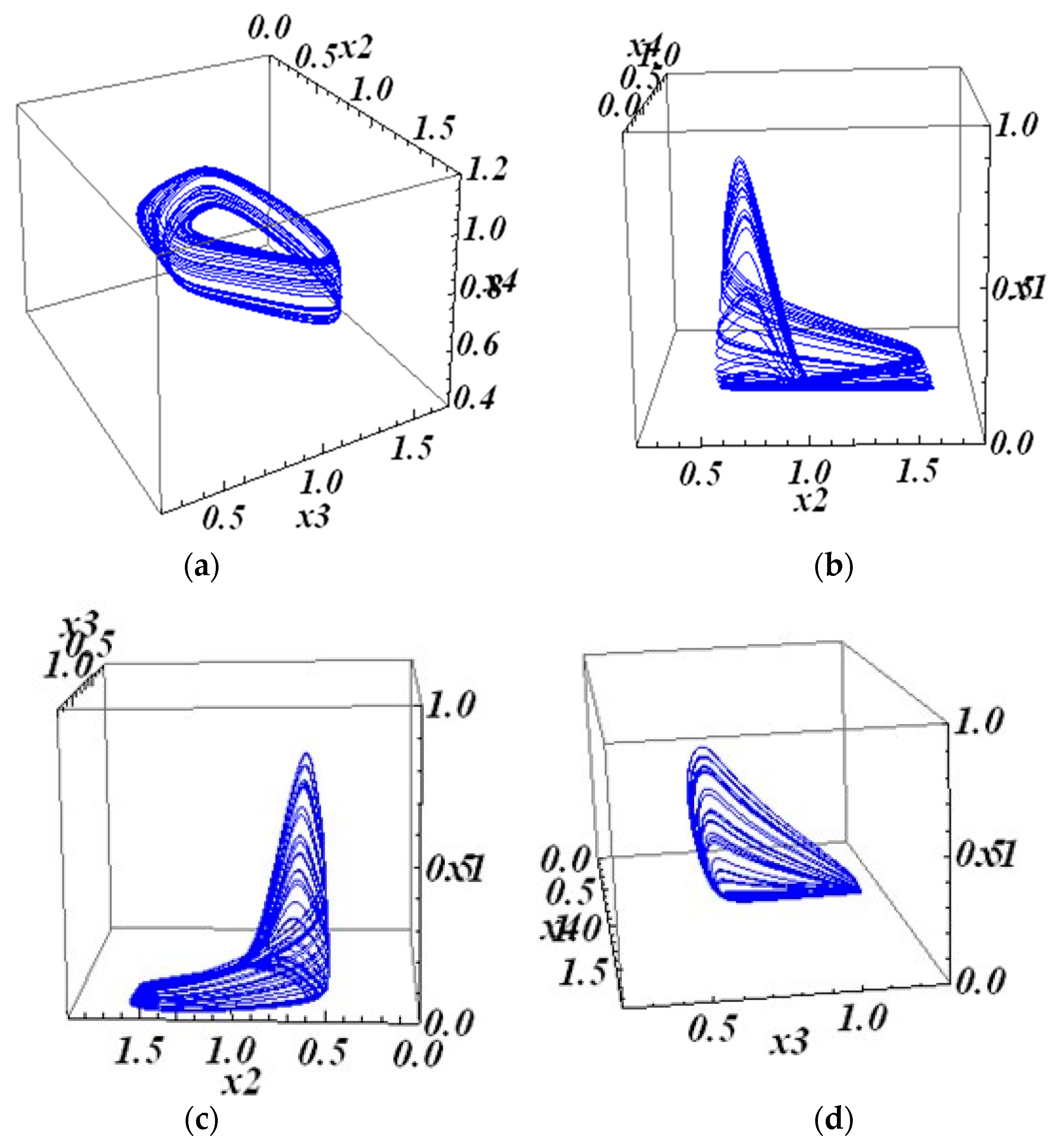
30]. More examples of that kind are provided. The second part of the article deals with the same subject but uses another approach. Previously obtained and published results on the 3D systems are used [
28,
29]. By adding suitable components to the 3D matrices used in the works, a 4D system is obtained, which has a visualizable 4D attractor. The behavior of solutions is chaotic. The Lyapunov curve analysis is provided. Useful information on the interpretation of the Lyapunov spectrum is in [
30]. Information on the best understanding of gene regulatory networks and chaotic behaviors of solutions can be found in [
31]. The properties of nonlinear systems and the role of attractors are covered in detail in [
32].
Despite being one of the most extensively studied areas in higher mathematics, the field of ordinary differential equations continues to expand significantly. This growth is driven by its widespread practical applications and its importance in education. The latter stems from the fact that linear and nonlinear ODE theory offers numerous instances of analytical problem solving, including the theory of linear ODE with constant coefficients.
Typically, ordinary differential equations (ODEs) cannot be solved analytically and require computational methods. To illustrate how attractors can emerge, we present two approaches, both utilizing numerical tools.
The second section covers preliminaries and basic knowledge of systems in the forms (1), (5), and (10). The third section examines four-dimensional systems with attractors that may exhibit sensitive dependence on initial conditions.
Section 4 provides new examples of 4D systems exhibiting chaotic solutions behavior.
2. Preliminaries
First, we consider the two-dimensional (2D) systems of ordinary differential equations (ODE) of the form
This system is the simplification [
17,
18] of the system that first appeared in the research by Wilson–Cowan [
16] on the dynamics of interactions between populations of excitatory and inhibitory neurons.
The right side contains two terms, a nonlinear one and a linear term. Without the nonlinear term, the system possesses only exponentially decreasing solutions, and it is not interesting (but physically explainable: no evolution without interactions).
Generally, μi are positive numbers, greater than 1, θi are adjustable parameters, and vi are positive, but in most cases they are set to 1. The parameters of the GRN have the following biological interpretations:
vi—degradation of the
i-th gene expression product;
wij—the connection weight or strength of control of gene
j on gene
i. Positive values of
wij signify activating influences, whereas negative values denote repressing influences;
θi—the impact of external stimuli on gene
i is reflected in its ability to modulate the gene’s responsiveness to activating or repressing factors [
26].
An invariant set in a dynamical system is a set of points in the system’s phase space that, once entered, the system will remain within for all future time steps. The invariant set for system (1) is the rectangle
Further, the
n-dimensional system
was used extensively in the mathematical modeling of gene regulatory networks and telecommunication networks [
33].
The basic facts about systems (1) and 3D version of system (2) can be found in [
24] and references therein, and in [
28], theorems 1 and 2.
Here are some of the facts:
- (1)
The above-defined set is invariant;
- (2)
In this set there is at least one critical point;
- (3)
The nullclines, defined by the equations
intersect only in the invariant set; therefore, all possible critical points are located in the invariant set.
Multiple examples of the study of the critical points of system (2) can be found in [
24,
28,
29].
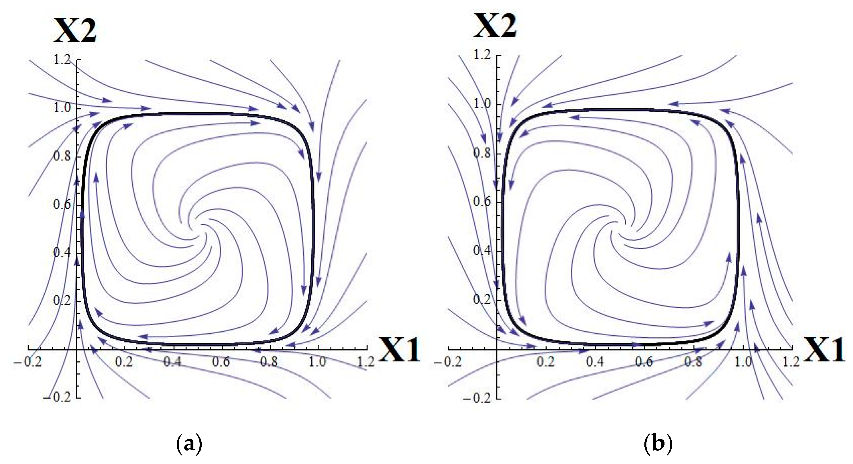
The behavior of trajectories of system (1) essentially depends on the coefficients
wij. There are three main modes of behavior, namely, activation, inhibition, and mixed case (which results in a rotating vector field) in system (1). They are characterized, respectively, by the following matrices:
5. Discussion
The study of gene networks is one of the important tasks of biomathematics. Systems of differential equations make it possible to model networks in motion and monitor their evolution. In this case, the problem becomes purely mathematical, but its tasks are corrected with the help of the biological data that are obtained. The system studied in this article is an interesting mathematical object. It is quasi-linear, i.e., it is the sum of linear and nonlinear parts. This property, together with the range of values of the nonlinearity (usually a sigmoidal function with the range (0, 1)), ensures the presence of an invariant set in the phase space and, as a result, the existence of an attractor(s). Attractors determine the future states of the system (and network). Attractors can be regular, the properties of which are well traced, and chaotic.
For this study, it is useful to construct examples of attractors for systems in question, where possible. In the first part of this work, such attractors are constructed as geometric objects obtained by combining systems of lower dimensions. In this case, well-readable systems of dimension 4 are obtained. This dimension was chosen for the study because it is the beginning of the non-visualizable field of study of gene systems. Several attractors have been obtained, the structure of which can be imagined by analyzing three-dimensional projections on the coordinate axes.
Attractors whose properties are close to chaotic were obtained, demonstrating the sensitivity of solutions to the initial data. An attractor has been received, the projections of which look like the union of closed curves in a 3-dimensional space. The tendency of the trajectories of the main 4-dimensional system to such an attractor depends on the initial data. Solutions tend to a selected attractor (based on the initial data). The biological counterpart of this behavior, tending to a selected periodic regime, should be studied and interpreted. These attractors are well visualized. In the second part of the work, two examples of chaotic attractors for 4-dimensional systems are constructed. For this, previously studied 3-dimensional systems with 3-dimensional chaotic attractors are used. The challenge is to augment these 3D systems to 4D systems in a nontrivial way, increasing the regulatory matrix W by one row and one column and saving the property of having a chaotic attractor. It is to be mentioned that other (concerning the elements of matrix W) parameters of the system are also involved in the process, for example, coefficients vi at the linear terms of a system.
There are some additional comments on the ongoing text. Examples of 3D systems that have a chaotic attractor were constructed in [
28,
29]. Paper [
28] uses the idea of the Chua circuit, which suggests that the system has 3 critical points (equilibria) of a certain type. The Chua circuit is a relatively simple-looking three-dimensional (3D) system that is almost linear with only one piecewise linear function on the right. The construction of a similarly organized 3D system of GRN-type (Genetic Regulatory System type) required work-consuming efforts. In [
29], the 3D chaotic system of the GRN type was constructed following the scheme proposed by Shilnikov. This scheme required the existence of a saddle-focus type equilibrium (critical point) with a certain balance between the characteristic numbers. The extension of these two 3D examples to the 4D examples with chaotic attractors was performed by adding a few elements to the matrices W, making it four-dimensional, and checking the result.
We suggest that our research advances the field in several directions. First, we have considered the parameter-dependent family of 4D systems, choosing afterward the appropriate system with the needed behavior. Second, we have considered 4D systems combined with two 2D systems with definite behavior of solutions. These two 2D systems were asked to have periodic solutions (limit cycles) with certain properties. In the second part of the work, the chaotic attractors were constructed for the 4D systems. This is a remarkable fact since even 3D examples of chaotic attractors for GRN-type systems are rare (for algebraic systems, the examples are many).
In our examples, two interacting subsystems, each representing a periodic process, are combined into a larger system. For high-dimensional systems where subsystems can be identified, a similar approach may approximate the larger system, potentially leading to more efficient analysis.
There are biological guidelines for selecting parameters in system (2). Altering μ impacts a gene’s individual property to accept inputs. Experimental data may offer insights into the type of interaction within a network or subsystems. Therefore, the matrix W, or an approximation, can be reconstructed. In a model, particularly for the 2D case, the activatory matrix W (where all elements are positive) generally results in stable equilibria. The same is true for the inhibition, but equilibria are located differently. In the mixed case, where there is a balance between activation and inhibition, stable periodic attractors may exist.
Periodic attractors were obtained in examples of the first part. They presumably may correspond to the repeating and rhythmic processes in real networks.
Lyapunov exponents relate to the chaotic behavior of solutions, or, at least, to sensitive dependence on the initial data. This goes beyond bistability and/or oscillatory behaviors. The bistability, or switching, of the behavior of genes has a natural mathematical counterpart, namely, certain bifurcations of solutions under the change in parameters. Mathematically, this can occur when the trajectory of a dynamical system crosses the border between basins of attraction of two neighboring attractors. The oscillations are a focus of our approach. Several kinds of oscillatory behaviors can be met even in 4D systems. Oscillations in GRN-type systems are very common. They are stimulated by a balance between activatory and inhibitory populations of genes.
Generally, GRN-type systems are stable (rough, structurally stable). Therefore, the influence of noise is not extensive and can be even neglected in many studies of GRN. The influence of unknown parameters can be hidden in the parameter θ. It can significantly affect the main properties of a system. On the other hand, this allows for management and control of the network, which is important for applications.


