Numerical Solution of Locally Loaded Volterra Integral Equations

Abstract

Loaded Volterra integral equations represent a novel class of integral equations that have attracted considerable attention in recent years due to their numerous applications in various fields of science and engineering. This class of Volterra integral equations is characterized by the presence of a loading function, which complicates their theoretical and numerical analysis. In this paper, we study Volterra equations with locally loaded integral operators. The existence and uniqueness of their solutions are examined. A collocation-type method for the approximate solution of such equations is proposed, based on piecewise linear approximation of the exact solution. To confirm the convergence of the method, several numerical results for solving model problems are provided.

1. Introduction

The concept of equations with loads was first introduced by Adam Nakhushev [1]. The study of various differential and integral equations with local and nonlocal loads enables the description of more complex processes where spatial and/or temporal localization and memory effects are significant.

In the monograph by Adam Nakhushev [1], a mathematical model is presented that describes the moisture transport process in porous soil media under certain idealized assumptions. The aforementioned model is formulated in terms of hyperbolic loaded differential equations and can be considered either as a characteristic Cauchy problem with non-smooth characteristic support or as a generalized Goursat problem [2,3].

In other works by Adam Nakhushev [4], methods for solving boundary value problems of mathematical physics and biology were developed, including modeling of particle transport processes [5]. Particular attention is given to problems of heat and mass transfer with finite speed of perturbation propagation and modeling of fluid filtration processes in porous media [6].

The work [7] is devoted to the Cauchy problem with a parameter perturbed by a linear functional, which generalizes the conventional load. The study examines conditions for the existence of trivial and nontrivial solutions in the neighborhood of a bifurcation point. In [8], the authors consider the Fredholm integral equation of the second kind with a load and construct solution methods for both regular and irregular cases. Previous research has also addressed the Hammerstein equation with a load [9], where the equation was studied through a series of nonlinear boundary value problems using Green’s function. Furthermore, ref. [10] establishes necessary and sufficient conditions for the spectra of loaded Sturm–Liouville operators, with the authors employing the term “frozen argument” instead of “load”.

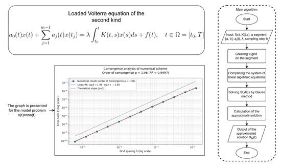
Let us consider, following the book [1], an integral equation of the form:

$$a_0\left(t\right)x\left(t\right)+\sum _{j=1}^{m-1}{a}_j\left(t\right)x\left(t_j\right)=\lambda {\int }_{t_0}^{t}K(t,s)x\left(s\right)ds+f\left(t\right),t\in \Omega =[t_0,T]$$

(1)

where $t_j,(j=1,2,\dots ,m-1)$ are defined fixed points of segment $[t_0,T]$, with $t_0<t_1<\cdots <t_{m-1}<t_m=T$; $\lambda$ is a constant parameter; $f\left(t\right),a_j\left(t\right)\in C_{[t_0,T]},j=\overline{0,m-1}$.

This equation is called either a linear one-dimensional loaded Volterra integral equation or simply a loaded Volterra integral equation (LVIE).

Let us write the Equation (1) in operator form:

$$Vx\left(t\right)=f\left(t\right),$$

where the operator V is defined as follows:

$$Vx\left(t\right)\equiv a_0\left(t\right)x\left(t\right)+\sum _{j=1}^{m-1}{a}_j\left(t\right)x\left(t_j\right)-\lambda {\int }_{t_0}^{t}K(t,s)x\left(s\right)ds.$$

The operator V is referred to as a locally loaded operatorbecause it incorporates a trace of the desired solution through its values $x\left(t_j\right)$ at certain points $t_j\in \Omega$, where $j=1,2,\dots ,m-1$.

As a footnote, to the best of our knowledge, the development of numerical methods for solving loaded equations has not yet been reported in the scientific literature.

2. Existence and Uniqueness of Solution

We consider Equation (1) in the space $C_{[t_0,T]}$, assuming that the input functions are continuous:

$$a_0\left(t\right)x\left(t\right)+\sum _{j=1}^{m-1}{a}_j\left(t\right)x\left(t_j\right)+\lambda {\int }_{t_0}^{t}K(t,s)x\left(s\right)ds=f\left(t\right),t\in \Omega =[t_0,T].$$

(2)

We also suppose that $a_0\left(t\right)\ne 0$. Then, without loss of generality, we set $a_0\left(t\right)\equiv 1$ in Equation (2). In this case, the kernel $K(s,t)$ possesses a resolvent $R(t,s,\lambda )$, which can be represented as a uniformly convergent series.

$$R(t,s,\lambda )=\lambda K_1(t,s)+{\lambda }^2{K}_2(t,s)+\cdots +{\lambda }^n{K}_n(t,s)+\dots$$

(3)

where $K_1(t,s)=K(t,s)$, $K_n(t,s)={\int }_s^t{K}_1(t,z)K_{n-1}(z,s)dz$ and the Equation (2) reduces to the following equation:

$$x(t,\lambda )+\sum _{j=1}^{m-1}{b}_j(t,\lambda )x(t_j,\lambda )=F(t,\lambda ),$$

(4)

where

$$\begin{array}{c}\hfill F(t,\lambda )=f\left(t\right)+{\int }_{t_0}^{t}R(t,s,\lambda )f\left(s\right)ds,\\ \hfill b_j(t,\lambda )=a_j\left(t\right)+{\int }_{t_0}^{t}R(t,s,\lambda )a_j\left(s\right)ds.\end{array}$$

Assuming, in (4), t successively equals $t_j,j=\overline{1,m}$, to define the load vector $\overline{c}={\left(x(t_1,\lambda ),\dots ,x(t_m,\lambda )\right)}^T$, we obtain a system of linear algebraic equations (SLAE):

$$A(t_j,\lambda )\overline{c}={\overline{d}}_{\lambda },$$

(5)

where the matrix $A(t_j,\lambda )\stackrel{def}{=}{[{\delta }_{ij}+b_j(t_i,\lambda )]}_{ij=\overline{1,m}}$, ${\delta }_{ij}$ is the Kronecker symbol, ${\overline{d}}_{\lambda }={\left(F(t_j,\lambda ),\dots ,F(t_m,\lambda )\right)}^T$.

If $detA\ne 0$, then the SLAE (5) has a single solution: $\overline{C}=A^{-1}{\overline{d}}_{\lambda }$. In this case, Equation (2) obviously has a single solution. Hence, the theorem follows:

Theorem 1. 

Suppose that in Equation (2), all the input functions are continuous and $a_0\left(t\right)\equiv 1$. Let $detA(t_j,\lambda )\ne 0$. Then the LVIE (2) has a single solution for all λ in class $C_{[t_0,T]}$.

For $\lambda =0$, the special case $A(t_j,0)={[{\delta }_{ij}+a_j\left(t_i\right)]}_{ij=\overline{1,m}}$.

If $A(t,0)\ne 0$, then by virtue of the continuity of the resolvent on $\lambda$ and $detA(t,\lambda )\ne 0$ when $\left|\lambda \right|detA(t,\lambda )\ne 0$ is small enough, the unambiguous solvability of LVIE (2) in $C_{[t_0,T]}$ follows.

If $detA(t,0)\ne 0$, then if $\lambda$ in Equation (2) is small enough, the load is uniquely determined and Equation (2) has a unique solution in $C_{[t_0,T]}$, determined from (4).

More interesting is the case where the equation contains a value $\lambda$ at which $detA(t,\lambda )=0$.

Theorem 2. 

If $detA(t,0)=0$ and $\mathit{rank}A(t,\lambda )=r$, then the corresponding homogeneous system will have $m-r$ linearly independent solutions. Correspondingly, the inhomogeneous system (5) with such λ will have no solutions if $\overline{d}\left(\lambda \right)$ is not orthogonal to the solution of the conjugate homogeneous system. If $\overline{d}\left(\lambda \right)$ is orthogonal to the solution of the conjugate homogeneous SLAE, then the inhomogeneous SLAE will have a parametric family of solutions depending on $m-r$ free parameters.

The following theorem follows from this result.

Theorem 3. 

Let $detA(t,{\lambda }_0)=0$, $\mathit{rank}A(t,{\lambda }_0)=r$ and the solvability conditions of the corresponding SLAE (5) be satisfied; then, integral Equation (2) has a solution dependent on $m-r$ arbitrary constants. If the solvability conditions of SLAE (5) are not fulfilled, then the integral Equation (2) has no solution in $C_{[t_0,T]}$.

3. Direct Numerical Method for the Solution of the Linear LVIE

In this paragraph, we construct a direct numerical method to solve (1) based on a piecewise linear approximation of the exact solution.

To discretize Equation (1), we denote by ${\Delta }_k,k=1,2,\dots ,m$, the segments $\Delta =\left[t_{k-1,t_k}\right]$ through ${\Delta }_k,k=1,2,\dots ,m$. Then, choosing a small enough sampling step h, we cover each of the segments ${\Delta }_k,k=1,2,\dots ,m$ with equally spaced nodes $s_k^l$, defined as follows:

$$s_k^l=t_{k-1}+{\displaystyle \frac{(t_k-t_{k-1})}{n_k}}·l,l=0,1,\dots ,n_k-1,n_k=\left[{\displaystyle \frac{t_k-t_{k-1}}{h}}\right]+1,s_m^{n_m}=t_m,$$

(6)

where $\left[s\right]$ is the integer part of s. The total number of grid nodes (6) is $N=1+{\displaystyle \sum _{k=1}^m}{n}_k$ nodes. For ease of writing, let us re-normalize by ${\tau }_i,i=0,1,\dots ,N,$ all nodes $s_k^l,k=1,2,\dots ,m,$ in ascending order.

Thus, we obtain a mesh of nodes ${\tau }_i,i=0,1,\dots ,N,$ consistent with the set of points $t_i,j=1,2,\dots ,m-1,$ defined in the original equation and satisfying the condition ${\displaystyle \underset{j=\overline{1,N}}{max}}({\tau }_i-{\tau }_{j-1})⩽h$.

We then look for an approximate solution $x_N\left(t\right)$ for Equation (1) in the form of a piecewise linear function constructed on a grid of nodes (6):

$$X_N\left(t\right)=x({\tau }_i-1)+{\displaystyle \frac{x\left({\tau }_i\right)-x\left({\tau }_{i-1}\right)}{{\tau }_i-{\tau }_{i-1}}}(t-{\tau }_{i-1}),t\in [{\tau }_{i-1},{\tau }_i],i=\overline{1,N}.$$

(7)

To determine the unknown values $x_i=x\left({\tau }_i\right),i=0,1,\dots ,N,$ we require the Equation (1) to be converted to equality at each of the grid points (6):

$$a_0\left({\tau }_i\right)x_i+\sum _{j=1}^{m-1}{a}_j\left({\tau }_i\right)x_{v_i}=\lambda {\int }_{t_0}^{{\tau }_i}K({\tau }_i,s)X_N\left(s\right)ds+f\left({\tau }_i\right),i=0,1,\dots ,N,$$

(8)

where $v_i$ is the number of the grid node ${\left\{{\tau }_i\right\}}_{i=0}^N$ coinciding with the value $t_j,j=1,2,\dots ,m-1.$ The numbers $v_i$ are determined and fixed during grid generation for a given value of the sampling step h.

Transform (8)

$$a_{0i}{x}_i+\sum _{j=1}^{m-1}{a}_{ji}{x}_{v_i}=\lambda \sum _{p=1}^i{\int }_{{\tau }_{p-1}}^{{\tau }_p}K({\tau }_i,s)\left(x_{p-1}+{\displaystyle \frac{x_p-x_{p-1}}{{\tau }_p-{\tau }_{p-1}}}(s-{\tau }_{p-1})\right)ds+f_i,$$

(9)

where $a_{ji}=a_j\left({\tau }_i\right),f_i=f\left({\tau }_i\right),j=0,1,\dots ,m-1,i=0,1,\dots ,N$.

Approximating the integrals in (9) by the mean rectangle formula, we arrive at a system of linear algebraic equations with respect to the unknown values $x_i,i=\overline{0,N}$, of the desired function:

$$a_{0i}{x}_i+\sum _{j=1}^{m-1}{a}_{ji}{x}_{v_i}-f_i={\displaystyle \frac{\lambda }{2}}\sum _{p=1}^i({\tau }_p-{\tau }_{p-1})K\left({\tau }_i,{\displaystyle \frac{{\tau }_{p-1}+{\tau }_p}{2}}\right)(x_{p-1}+x_p),i=\overline{0,N}.$$

(10)

For (10), abbreviated notations were introduced to ensure conciseness of the expression:

$$J_p{x}_{p-1}+J_p{x}_p={\displaystyle \frac{\lambda }{2}}\sum _{p=1}^i({\tau }_p-{\tau }_{p-1})K\left({\tau }_p,{\displaystyle \frac{{\tau }_{p-1}+{\tau }_p}{2}}\right)(x_{p-1}+x_p),p=1,2,\dots ,i.$$

Let us also introduce an auxiliary notation for the left part of the SLAE (10):

$$H_i{x}_{v_i}=\sum _{j=1}^{m-1}{a}_{ji}{x}_{v_i}=(a_{1i}+a_{2i}+\cdots +a_{(m-1)i})x_{v_i},i=\overline{0,N}.$$

Then the system of Equations (10) will take the following form:

$$\left\{\begin{array}{c}{a}_{00}{x}_0+H_0{x}_{v_0}-f_0=0\hfill \\ -J_1{x}_0+(a_{01}-J_1)x_1+H_1{x}_{v_1}-f_1=0\hfill \\ \cdots \cdots \cdots \cdots \cdots \cdots \cdots \cdots \cdots \cdots \cdots \cdots \cdots \cdots \cdots \hfill \\ -J_1{x}_0+(-J_1-J_2)x_1+\cdots +(-J_{i-2}-J_{i-1})x_{i-1}+\hfill \\ +(a_{0i}-J_i)x_i+H_i{x}_{v_i}-f_i=0.\hfill \end{array}\right.$$

(11)

Suppose that the solution of the well-conditioned system of linear algebraic Equation (11) is obtained with sufficient accuracy—for example, by using an exact method whose error is limited solely by computational precision. Then, the following estimate for the error of the proposed numerical method can be established:

$${\epsilon }_h={\parallel X_N\left(t\right)-x\left(t\right)\parallel }_{C_{[t_0,T]}}=\mathcal{O}\left({\displaystyle \frac{1}{N^2}}\right)=\mathcal{O}\left(h^2\right).$$

(12)

4. Numerical Experiments

In order to demonstrate the performance of the proposed numerical method for solving the loaded Volterra integral equations, calculations are performed for two model problems. The algorithm is implemented in the C++ programming language, and for solving the system of linear algebraic equations, the Gauss–Jordan method with selection of the maximum element is applied.

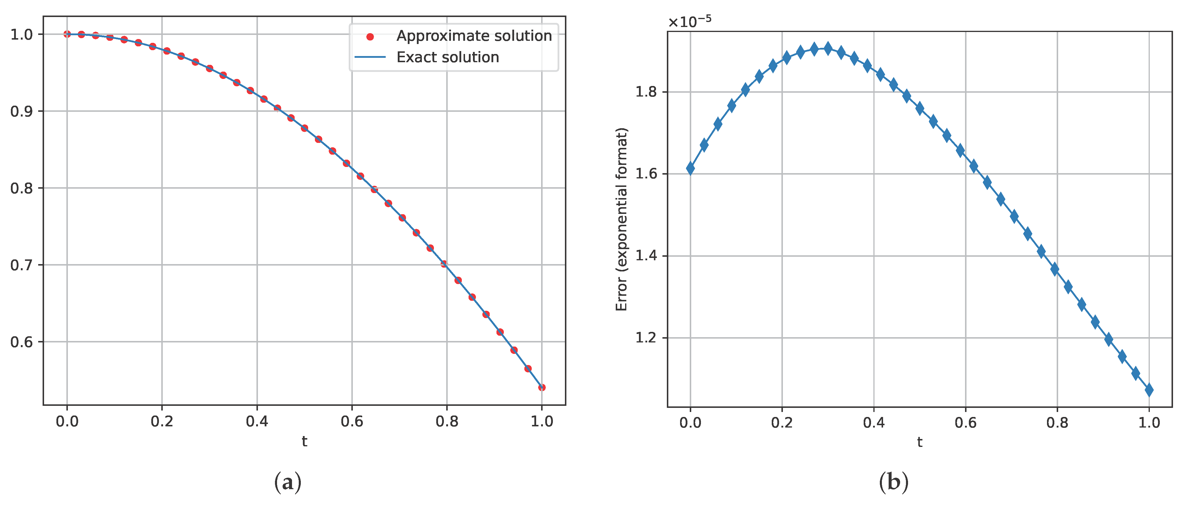
4.1. Model Problem 1

Consider Equation (1) with the following parameters:

$$\begin{array}{c}t\in [t_0,T]=[0,1];m=3;t_1={\displaystyle \frac{3}{10}};t_2={\displaystyle \frac{1}{2}};\lambda ={\displaystyle \frac{1}{4}};\\ a_0\left(t\right)=t^2+1;a_1\left(t\right)=1-t^3;a_2\left(t\right)=t-2;K(t,s)=t-2s^2;\\ f\left(t\right)=(t^2+1)cost+(1-t^3)cos\left({\displaystyle \frac{3}{10}}\right)+(t-2)cos\left({\displaystyle \frac{1}{2}}\right)+{\displaystyle \frac{t^2}{2}}sint-{\displaystyle \frac{t}{4}}sint+tcost-sint.\end{array}$$

The exact solution in this case is the function $x\left(t\right)=cos\left(t\right)$.

Table 1. The magnitude of the error and order of convergence.

h	1/8	1/16	1/32	1/64	1/128	1/256
${\epsilon }_h$	2.20 × 10−4	6.99 × 10−5	1.91 × 10−5	5.04 × 10−6	1.30 × 10−6	3.30 × 10−7
r	—	1.65	1.88	1.92	1.96	1.98

and

Table 2. The magnitude of the error and order of convergence.

h	1/512	1/1024	1/2048	1/4096	1/8192	1/16,384
${\epsilon }_h$	8.31 × 10−8	2.09 × 10−8	5.23 × 10−9	1.31 × 10−9	3.27 × 10−10	8.18 × 10−11
r	1.99	1.99	1.93	2.07	2.00	2.00

show the results of the method for different steps, where the following notations are used: h is the sampling step, ${\epsilon }_h={\parallel X_N\left(t\right)-x\left(t\right)\parallel }_{C_{[t_0,T]}}$ is the error, and $r={\displaystyle \frac{ln\frac{{\epsilon }_{h_{k-1}}}{{\epsilon }_{h_k}}}{ln\frac{h_{k-1}}{h_k}}}$ is the order of convergence.

Figure 1 illustrates the proximity of the exact and approximate solution of model problem 1.

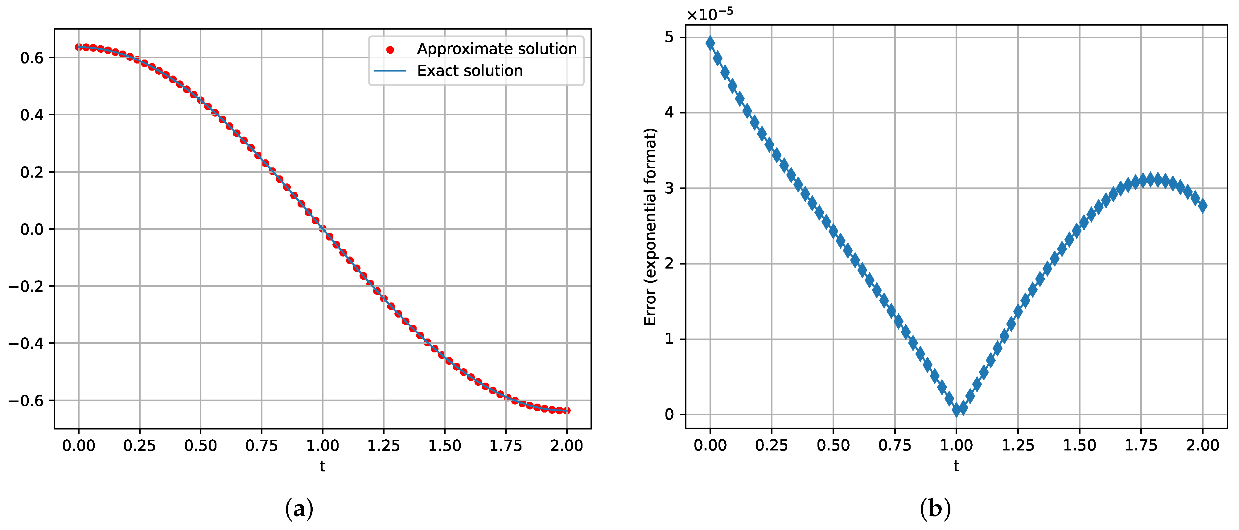
4.2. Model Problem 2

Consider Equation (1) with the following parameters:

$$\begin{array}{c}t\in [t_0,T]=[0,2];m=6;t_1={\displaystyle \frac{3}{10}};t_2={\displaystyle \frac{1}{2}};t_3=1;t_4={\displaystyle \frac{5}{4}};t_5={\displaystyle \frac{5}{3}};\\ \lambda ={\displaystyle \frac{1}{6}};K(t,s)=t-2s^2;a_0\left(t\right)={\displaystyle \frac{2+t}{3}};a_1\left(t\right)=t^3-{\displaystyle \frac{1}{2}};\\ a_2\left(t\right)=2t-t^2;a_3\left(t\right)=4t^3;a_4\left(t\right)=t-2t;a_5\left(t\right)={\displaystyle \frac{t}{2}}+1;\\ f\left(t\right)={\displaystyle \frac{2\left(\frac{2+t}{3}\right)cos\left(\frac{\pi t}{2}\right)}{\pi }}+{\displaystyle \frac{2(t^3-\frac{1}{2})cos\left(\frac{3\pi }{20}\right)}{\pi }}+{\displaystyle \frac{(-t^2+2t)\sqrt{2}}{\pi }}\\ -{\displaystyle \frac{2(t-2^t)cos\left(\frac{3\pi }{8}\right)}{\pi }}-{\displaystyle \frac{(\frac{t}{2}+1)\sqrt{3}}{\pi }}-{\displaystyle \frac{2e^t(sin\left(\frac{\pi t}{2}\right)\pi t+2cos\left(\frac{\pi t}{2}\right)-2)}{3{\pi }^3}}\end{array}$$

The exact solution in this case is the function $x\left(t\right)={\displaystyle \frac{2}{\pi }}cos\left({\displaystyle \frac{\pi t}{T}}\right)$.

Table 3. The magnitude of the error and order of convergence.

h	1/8	1/16	1/32	1/64	1/128
${\epsilon }_h$	5.49 × 10−4	1.88 × 10−4	4.92 × 10−5	1.35 × 10−5	3.43 × 10−6
r	—	1.55	1.93	1.87	1.98

and

Table 4. The magnitude of the error and order of convergence.

h	1/256	1/512	1/1024	1/2048	1/4096
${\epsilon }_h$	8.80 × 10−7	2.21 × 10−7	5.56 × 10−8	1.39 × 10−8	3.48 × 10−9
r	1.96	1.99	1.99	1.93	2.07

show the results of the method for different steps, using the same notation.

Figure 2 shows the exact and approximate solution of model problem 2.

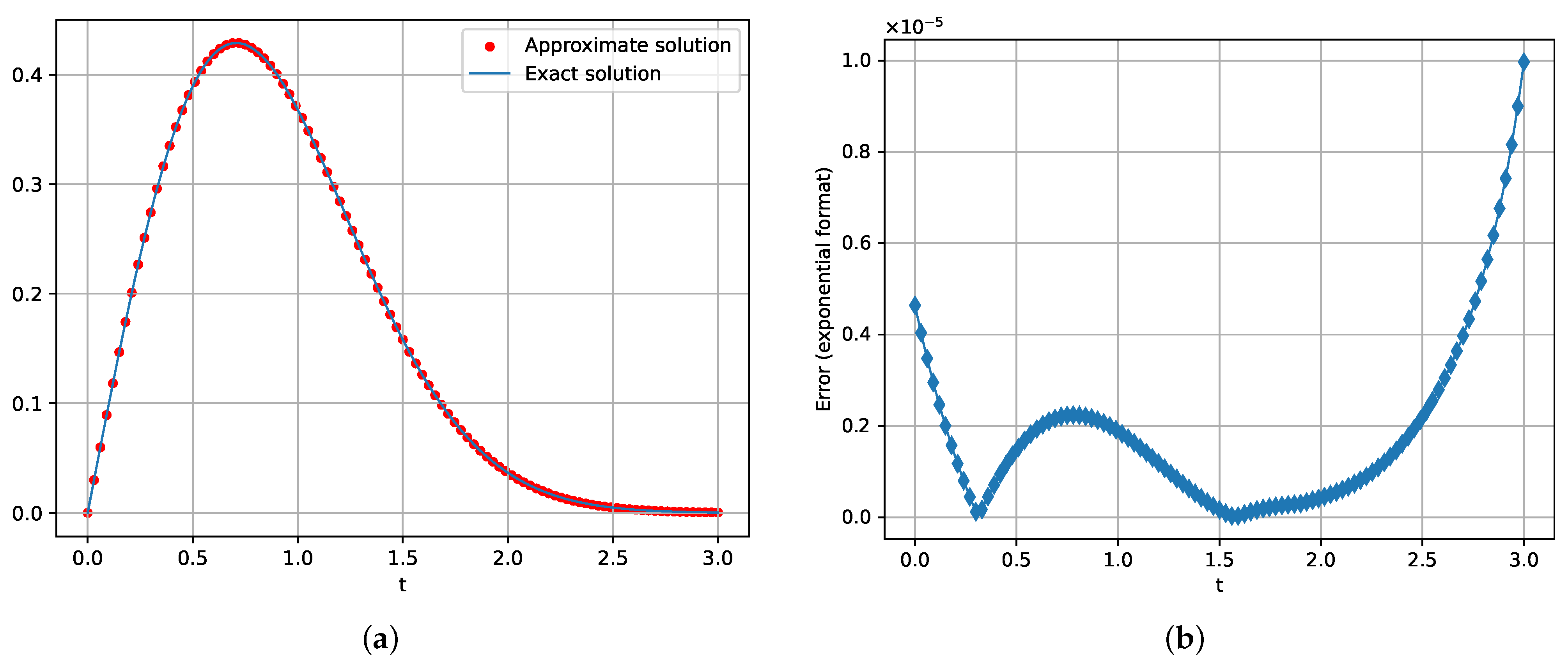
4.3. Model Problem 3

Consider Equation (1) with the following parameters:

$$\begin{array}{c}t\in [t_0,T]=[0,3];m=6;t_1={\displaystyle \frac{6}{10}};t_2={\displaystyle \frac{12}{10}};t_3={\displaystyle \frac{15}{10}};t_4={\displaystyle \frac{19}{10}};t_5={\displaystyle \frac{24}{10}};\\ \lambda ={\displaystyle \frac{1}{8}};K(t,s)=2s-s^2+t^3;\\ a_0\left(t\right)=2sin\left(t\right);a_1\left(t\right)=t;a_2\left(t\right)=4cos\left(t\right);a_3\left(t\right)=e^t;a_4\left(t\right)=5^t+100t;a_5\left(t\right)=t^4+t;\\ f\left(t\right)=2sin\left(t\right)t{e}^{-t^2}+{\displaystyle \frac{3e^t{e}^{-\frac{9}{4}}}{2}}+{\displaystyle \frac{3t{e}^{-\frac{9}{25}}+24cos\left(t\right)e^{-\frac{36}{25}}+12(t^4+t)e^{-\frac{144}{25}}}{5}}+\\ +{\displaystyle \frac{19(5^t+100t)e^{-\frac{361}{100}}}{10}}-{\displaystyle \frac{(t^3{e}^{t^2}+\sqrt{\pi }\mathrm{erf}\left(t\right)e^{t^2}-t^3+t^2-e^{t^2}-2t+1)e^{-t^2}}{16}}\end{array}$$

The exact solution in this case is the function $x\left(t\right)=t{e}^{-t^2}$.

Table 5. The magnitude of the error and order of convergence.

h	1/8	1/16	1/32	1/64	1/128
${\epsilon }_h$	8.54 × 10−5	3.22 × 10−5	9.96 × 10−6	2.76 × 10−6	7.21 × 10−7
r	—	1.41	1.69	1.85	1.93

and

Table 6. The magnitude of the error and order of convergence.

h	1/256	1/512	1/1024	1/2048
${\epsilon }_h$	1.85 × 10−7	4.68 × 10−8	1.18 × 10−8	2.95 × 10−9
r	1.97	1.98	1.99	1.93

show the results of the method for different steps, using the same notation.

Figure 3 shows the exact and approximate solution of model problem 3.

The obtained computational results reveal a consistent trend: as the step size decreases, the error also decreases in all three cases. This observation is further supported by the calculated empirical convergence rate coefficient.

In the first two model examples, the convergence rate approaches the second order ($r\approx 2$). However, in the third model example, the method initially exhibits a slower convergence rate ($r\approx 1.4–1.7$) before eventually reaching second-order convergence. This behavior is likely attributable to the specific initial conditions of the third model problem.

Error distribution plots were generated for each example, demonstrating a general reduction in error across the entire interval. However, the third model problem presents an exception: while the method still converges, the maximum error occurs at the end of the interval, indicating a deviation from the trend observed in the other cases.

5. Conclusions

In this paper, linear integral Volterra equations of the form (1) with a loaded integral operator are investigated. A numerical method of the collocation type is constructed based on piecewise linear approximation of exact solutions and designed for such equations with continuous input data. The numerical method was tested on a number of model problems, two of which are given in Section 4. The obtained results confirm the effectiveness of the method and the given theoretical estimate. If there is additional information concerning the smoothness of the functions included in the equation, more accurate approximation tools can be used to approximate the solution and integrals when forming the matrix of the system. The authors plan to further develop a spline collocation method (similar to the one proposed in [11]) for linear and nonlinear integral equations with load.

The current study does not address the stability analysis of the proposed method. Numerical experiments reveal that the method demonstrates sensitivity to input perturbations, becoming unstable for noise levels exceeding $\sigma >{10}^{-4}$. Subsequent research by the authors will explore this aspect and evaluate the method’s application in practical cases.

References

- Nakhushev, A.M. Loaded Equations and Their Application, 1st ed.; Research Institute of Invitational Mathematics and Automation KBNTs RAS, Nauka: Moscow, Russia, 2012; pp. 8–23. [Google Scholar]
- Mamedov, I.G. A new type Goursat problem for loaded Volterra-hyperbolic integro-differential vector equations of fourth order with non-smooth matrix coefficients. Proc. Natl. Acad. Sci. Azerbaijan 2006, 26, 74–79. [Google Scholar]
- Mamedov, I.G. The problem of optimal control in processes described by a nonlocal problem with loadings for the hyperbolic integro-differential equation. Proc. Natl. Acad. Sci. Azerbaijan 2004, 24, 74–79. [Google Scholar]
- Nakhushev, A.M. The Equations of Mathematical Biology, 1st ed.; High School: Moscow, Russia, 1995; pp. 102–125. [Google Scholar]
- Wiener, J.; Debnath, L. A survey of partial differential equations with piecewise continuous arguments. Internet J. Math. Math. Scz. 1995, 18, 209–228. [Google Scholar] [CrossRef]
- Shkhanukov, M.H. On some boundary value problems for the third order equation arising at modelling of liquid filtration in porous media. Differ. Equ. 1982, 18, 689–699. [Google Scholar]
- Dreglea Sidorov, L.R.; Sidorov, N. Cauchy problem with a parameter perturbed by a linear functional. Proc. Sci. Technol. Mod. Math. Appl. Themat. Rev. 2024, 237, 10–17. [Google Scholar]
- Dreglea Sidorov, L.R.; Sidorov, N.; Sidorov, D. The linear Fredholm integral equations with functionals and parameters. Bul. Acad. Ştiinţe Repub. Mold. Mat. 2023, 2, 83–91. [Google Scholar] [CrossRef]
- Sidorov, N.A.; Dreglea Sidorov, L.R.D. On the Solution of Hammerstein Integral Equations with Loads and Bifurcation Parameters. Bull. Irkutsk. State Univ. Ser. Math. 2023, 43, 78–90. [Google Scholar] [CrossRef]
- Kuznetsova, M. Necessary and sufficient conditions for the spectra of the Sturm—Liouville operators with frozen argument. Appl. Math. Lett. 2022, 131, 108035. [Google Scholar] [CrossRef]
- Tynda, A.; Noeiaghdam, S.; Sidorov, D. Polynomial spline collocation method for solving weakly regular Molterra integral equations of the first kind. Bull. Irkutsk. State Univ. Ser. Math. 2022, 39, 62–79. [Google Scholar]