Abstract
The decomposition of a signal is a fundamental tool in many fields of research, including signal processing, geophysics, astrophysics, engineering, medicine, and many more. By breaking down complex signals into simpler oscillatory components, we can enhance the understanding and processing of the data, unveiling hidden information contained in them. Traditional methods, such as Fourier analysis and wavelet transforms, which are effective in handling mono-dimensional stationary signals, struggle with non-stationary datasets and they require the selection of predefined basis functions. In contrast, the empirical mode decomposition (EMD) method and its variants, such as Iterative Filtering (IF), have emerged as effective non-linear approaches, adapting to signals without any need for a priori assumptions. To accelerate these methods, the Fast Iterative Filtering (FIF) algorithm was developed, and further extensions, such as Multivariate FIF (MvFIF) and Multidimensional FIF (FIF2), have been proposed to handle higher-dimensional data. In this work, we introduce the Multidimensional and Multivariate Fast Iterative Filtering (MdMvFIF) technique, an innovative method that extends FIF to handle data that varies simultaneously in space and time, like the ones sampled using sensor arrays. This new algorithm is capable of extracting Intrinsic Mode Functions (IMFs) from complex signals that vary in both space and time, overcoming limitations found in prior methods. The potentiality of the proposed method is demonstrated through applications to artificial and real-life signals, highlighting its versatility and effectiveness in decomposing multidimensional and multivariate non-stationary signals. The MdMvFIF method offers a powerful tool for advanced signal analysis across many scientific and engineering disciplines.
1. Introduction
Signal decomposition of 1D and higher-dimensional datasets plays an important role in applied mathematics and signal processing, and it has many applications in data analysis [1,2,3,4], image processing [5,6,7], machine learning [8,9,10], geophysics [11,12,13], communications [14,15,16], and many other fields. Decomposing complicated signals into simpler oscillatory components can help in understanding the underlying structures and enable efficient data representation [17,18], noise reduction [17,19], and feature extraction [18,20,21]. Customary decomposition techniques like Fourier analysis and wavelet transforms effectively process one-dimensional signals and methods that can handle multidimensional and multivariate signals are increasingly important as real-world data grows in complication. However, these methods have limitations. Fourier-based techniques [22] assume the stationarity of the signal, whereas wavelet-based methods [23] require the a priori selection of a proper basis to be used. Furthermore, both approaches are linear in nature.
To address these limitations, in 1998, the pioneering empirical mode decomposition method was published [23]. EMD separates signals into their oscillatory components, known as Intrinsic Mode Functions (IMFs), by iteratively subtracting local averages defined by the envelopes connecting the maxima and minima of the signal. While effective in many applications, EMD and derived algorithms suffer from several limitations, including their reliance on envelope interpolation and the lack of a rigorous mathematical framework. For these reasons, in the last two decades, many alternative non-linear methods, which require a priori selection of the base to be used as common in every technique based on optimization, have been developed, like, for instance, the sparse Time Frequency representation [24], the geometric mode decomposition [25], the symplectic geometry mode decomposition [26,27], the empirical wavelet transform [28], and the variational mode decomposition [29,30]. Among them, the only one based on iteration, and therefore, not requiring any a priori assumption on the signal under investigation, like the number of IMFs contained in the signal or the basis to be used in the decomposition, is the Iterative Filtering (IF) method.
The Iterative Filtering (IF) algorithm’s structure is based on EMD’s ones, with the key difference in the way the signal’s moving average is computed. IF computes the moving average as the convolution of the signal f with a compactly supported filter or window w, instead of relying on the average of two envelopes, like in the EMD
where L represents the filter length, or half-support of the filter function w. Unlike traditional approaches, IF determines L adaptively based on the signal itself. For instance, as suggested in [17,31], L can be computed using the relative distances between subsequent extrema of the signal. This self-adaptive approach makes IF inherently non-linear, enabling it to adjust to the signal’s characteristics. Building on IF, the Fast Iterative Filtering (FIF) algorithm was developed to accelerate the decomposition process using the Fast Fourier Transform (FFT). FIF preserves the adaptive nature of IF while significantly reducing computational costs, making it suitable for high-dimensional data. In addition to its speed, FIF introduces the ability to select filter properties, such as the Fokker–Planck filter, which ensures smoothness and compact support.
In recent years, FIF has been extended to handle increasingly complex datasets, leading to the development of the Multivariate Fast Iterative Filtering (MvFIF) [32], Multidimensional Iterative Filtering (MIF) [33], and Multidimensional Fast Iterative Filtering (FIF2) [34] algorithms. These extensions enable the decomposition of multichannel signals and multidimensional data, respectively, adapting the principles of FIF to higher dimensional and temporal domains.
In this work, we introduce the Multidimensional and Multivariate Fast Iterative Filtering (MdMvFIF) technique which extends FIF to handle datasets that vary, at the same time, across space and time, and we present its application to handle artificial and real-life signals. To the best of our knowledge, this algorithm is the first of its kind. There have been few algorithms proposed so far in the literature for the decomposition of non-stationary signals defined in higher dimensions, possibly including also time, like the fast and adaptive empirical mode decomposition for multidimensional, multivariate signals (FA-MVEMD) [35] and the fast empirical mode decomposition method for multidimensional signals based on serialization (Serial-EMD) [36]. However, these methods handle time as if it were an extra spatial dimension and not as a dimension per se. This is fine as far as the time and space variations are separated. However, in real-life signals, this is usually not the case, and space and time variations are tangled, for instance in plasma density simulations [37]. Furthermore, if we want to remove different ranges of frequencies from time and space it will be impossible to do it with these algorithms. This is a common problem in applications. Think, for instance, of what is shown in [38]. In that work, the datasets need to be filtered in high frequency in time and low frequency in space or vice versa. This task cannot be accomplished with the algorithms proposed so far in the literature.
The rest of this work is organized as follows. We first briefly recall the multidimensional and the multivariate extensions of the Fast Iterative Filtering. Then, in Section 2, we present the proposed approach to handle data that are, at the same time, multidimensional and multivariate. Next, in Section 3, we present a few examples of applications to both artificial and real-life signals. Finally, we derive the conclusions in Section 4.
1.1. Multidimensional Fast Iterative Filtering
The Multidimensional Fast Iterative Filtering (FIF2) method allows us to decompose an n-dimensional signal into simple oscillatory components, called Intrinsic Mode Functions (IMFs), by approximating the higher dimensional moving average of f and iteratively subtracting it. Unlike the empirical mode decomposition (EMD), which relies on maxima and minima envelopes, FIF computes the moving average using a convolution of f with a multidimensional filter w, defined as a non-negative, even, and continuous function compactly supported in , with .
The algorithm assumes the periodicity of f at its boundaries, a limitation that can be addressed by pre-extending the signal to enforce periodicity [39]. The filter support size is calculated based on the signal’s characteristics, such as its extrema count or Fourier spectrum. This signal-dependent determination of makes FIF2 non-linear and ensures adaptive decomposition.
The FIF2 method involves two nested loops:
- Inner Loop: Extracts an IMF by iteratively applying the filtering process until a stopping criterion is met.
- Outer Loop: Applies the same process to the residual signal, producing successive IMFs until the residual has at most one local extremum, classifying it as a trend signal.
The computational complexity of FIF2 is , where m is the maximum among all dimensions of the signal under investigation. The method’s robustness and efficiency are enhanced by choosing a Generalized Fokker–Planck filter [33]. These filters belong to the space (i.e., the set of infinitely differentiable functions on ) and are compactly supported. The of the filter ensures that, when we apply it iteratively, we do not reduce the smoothness of the signal. Moreover, the compact support guarantees that the computed average is truly local. To the best of our knowledge, generalized Fokker–Planck (F-P) filters are the only filters that possess both smoothness and a compact support. These filters are widely employed in various practical applications, such as [40,41,42,43]. This method has been proven to be a priori convergent and stable [33,34,44].
1.2. Multivariate Fast Iterative Filtering
The Multivariate Fast Iterative Filtering (MvFIF) method extends FIF to handle n-dimensional signals [32]. For a signal which is varying over time , the algorithm computes a single filter length L and applies the 1D FIF to each channel.
To determine L, the signal is treated as a sequence of column vectors rotating in . The filter length is derived from the angle of rotation between consecutive vectors:
where the symbol · denotes dot product between two vectors, and represents a norm of the space. The filter length is set as twice the average distance between extrema in . This approach ensures that the decomposition adapts to the highest frequency rotations embedded in the signal. The computational complexity of MvFIF is , where n is the number of channels and m is the signal length. Also, this method has been proven a priori convergent and stable [32].
2. Proposed Approach
Given a discrete n-dimensional signal f that varies over time , we want to decompose it into IMFs. We propose in this work what we call the Multidimensional and Multivariate Fast Iterative Filtering (MdMvFIF) algorithm. The idea is to extract an IMF in space and one in time iteratively until the signal does not contain any oscillations anymore, both in space and time. In particular, for , fixed, we start estimating the filter support to be applied to , as performed in the FIF2 algorithm. We estimate for every time instant t and then compute
which will be the support of the filter we apply to all space tensors for every fixed . It is important to underline that the optimal computation of the filter support in 2D and higher dimensional spaces is currently an open problem [33,34]. Solving this problem is out of the scope of the present work. In the numerical section, to compute the support , we rely on what was performed for the FIF2 algorithm [34]. Furthermore, we select a Generalized Fokker–Planck filter , as in [33], as a filter function and we impose its support to be . Then, we convolve it with the signal to produce its moving average . We then subtract it from the signal and iterate the procedure producing , for , until a stopping criterion is satisfied.
Regarding the stopping criterion, there are many possible options. One way of doing it, as mentioned in [17,31] for the monodimensional case, is to consider the relative change in and discontinue the inner loop at a certain as soon as a prefixed threshold of is reached. This can be expressed as
The previous steps will produce the first estimate of the first IMF in space, . To speed up calculations, we can compute convolution in the frequency domain, where it becomes a simple product. This is made possible, with low computational complexity, thanks to the FFT method. To give the measure of the acceleration induced by this alternative approach, we can consider that if the signal under investigation is and after discretization is a cube of dimension , then the computational complexity of the convolution passes from in time domain to if performed in the frequency domain via FFT.
After computing the first IMF in space, we can subtract it from the signal to obtain a new signal . We can then compute the signal moving average over time. To do so, we apply a multivariate approach, similar to the Multivariate Fast Iterative Filtering (MvFIF) method [32]. We consider now the vector obtained by fixing and combining the signal f and the time stamp t, and we measure the vector rotations as the time passes
We point out that in this formula, differently from previous approaches, the time variability is now taken into account as an variable [32]. We can now define the filter length L of a Fokker–Planck filter that we want to convolve with the signal to obtain its moving average. L, which is the half support size of the filter, can be computed as the double average distance between subsequent extrema in the signal . We point out that this approach is very natural if we consider a multivariate IMF as a vector in rotating around the time axis. Computing the double average distance between subsequent extrema in allows us to estimate the average scale of the highest frequency rotations embedded in this given signal.
We can now convolve the computed filter with the signal to produce its moving average . We then subtract it from the signal and iterate the procedure, producing , for , until the stopping criterion (4) is satisfied. Also, in this case, we can consider the relative change in and discontinue the inner loop at a certain as soon as a prefixed threshold is reached. This is how we produce the first estimate of the first IMF in time, . If we subtract this other first IMF from the signal, we obtain a new signal , and we can repeat the entire previous procedure to extract the subsequent IMFs in space and time. We iterate this procedure until there are no more oscillations left both in space and time.
The convergence and stability of this newly proposed method follow directly from the convergence and stability of the FIF2 and MvFIF algorithms.
The pseudo-code of MdMvFIF is given in Algorithm 1 and a MATLAB implementation is available online (http://www.cicone.com).
When the space and time variations are separated, i.e., in the vector the variation over time t is the same for every point , we could further accelerate calculations via the convolution of the data tensor with an dimensional filter. We call this algorithm the Space-Time Fast Iterative Filtering (ST_FIF), the pseudo-code of which is given in Algorithm 2.
In this pseudo-code, DFT and iDFT stand for Discrete Fourier Transform and inverse DFT, respectively, whereas represents the i-th IMF.
ST_FIF produces a decomposition that is somehow equivalent to what is also performed in the fast and adaptive empirical mode decomposition for multidimensional, multivariate signals (FA-MVEMD) [35] and the fast empirical mode decomposition method for multidimensional signals based on serialization (Serial-EMD) [36]. As we mentioned in the introduction, these methods can be applied under the assumption that the space and time variations in the data are not tangled; otherwise, the decompositions produced will contain artifacts. Furthermore, these methods have a second limitation—as also explained in the introduction, the IMFs produced contain time and space frequencies combined together. If we want to filter different frequency ranges for time and space it will not be possible with this algorithm. For these reasons, in this work, we focus only on implementing the first algorithm and show in the next section a few applications for synthetic and real-life signals.
| Algorithm 1 Multidimensional and Multivariate Fast Iterative Filtering IMFs = MdMvFIF |
|
| Algorithm 2 Space Time Fast Iterative Filtering IMFs = ST_FIF |
|
3. Numerical Examples
To show the abilities of the MdMvFIF algorithm in handling data, we apply it to two artificial signals, a simulation of plasma density and two real-life datasets. For the sake of simplicity, especially in plotting results, in the following, we focus on signals that are 2D in space; x and y will define the two-dimensional spatial domain, which evolves over time, denoted by t, producing 3D data cubes. It is important to point out that a data cube with 2D spatial and 1D temporal dimensions may contain active frequencies— in space and in time. As a result, the MdMvFIF technique will produce IMFs plus a trend: p IMFs capturing the spatial frequencies, and the remaining q capturing the temporal frequencies. Each spatial IMF corresponds to a single active spatial frequency, while each temporal IMF corresponds to a single active temporal frequency. The proposed approach can handle signals of any dimension in space plus time.
MdMvFIF, like all signal analysis techniques, requires careful handling of boundaries [39]. This work focuses on the development of the method itself; therefore, in the following examples, we assume ideal boundary management and defer a detailed analysis of boundary effects to future work. For this same reason, in all subsequent examples, when we plot temporal decomposition, we select coordinate points which are away from the domain boundaries to eliminate any possible edge effects and minimize boundary-related artifacts.
In the artificial examples presented, spatial and temporal variations are separable. This means that the temporal evolution is the same at each spatial location. This simplification is intended to ease the interpretation of results, considering that, like EMD and related approaches, the MdMvFIF method does not produce a unique decomposition [45]. In contrast, for real data, the potential presence of mixed space-time modes cannot be ruled out in general, and the absence of ground truths makes it impossible to assess if the IMFs are accurately separated. Hence, from now on, we make the assumption that no significant space-time mixing is present in the data under investigation and interpret the results accordingly. All results presented in the following examples were generated using MATLAB R2023b 64 bit, and the source code is available online (http://www.cicone.com).
3.1. First Artificial Example
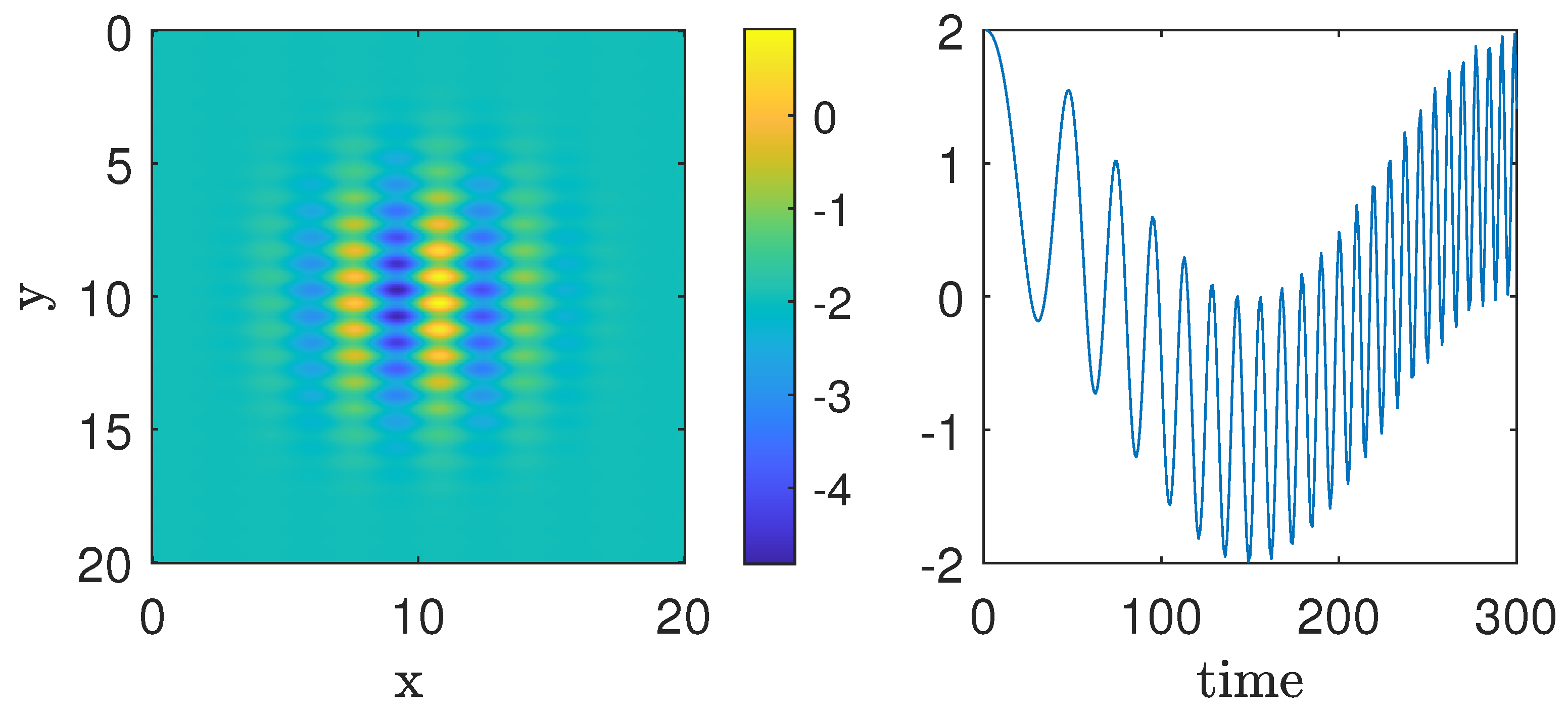
In this first example, we have a signal containing two non-stationary frequencies active in space and two stationary frequencies active in time. The goal of the decomposition is to separate these different types of oscillatory content into distinct IMFs. The data are shown in Figure 1 and Figure 2. In Figure 1, the left panel shows the signal at time on a two-dimensional spatial grid, where the x and y axes represent spatial coordinates, and the color gradient (ranging from blue to yellow) indicates signal intensity at each location. The right panel displays the time evolution of the signal at the fixed position ; the plot represents the variation in signal intensity over time, with the color scale again indicating amplitude.
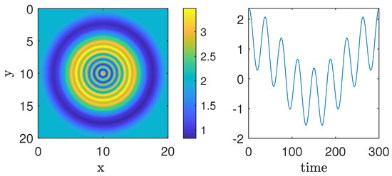
Figure 1.
Example 1. (Left panel): Signal at time . (Right panel): Time evolution for position .
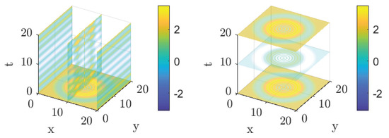
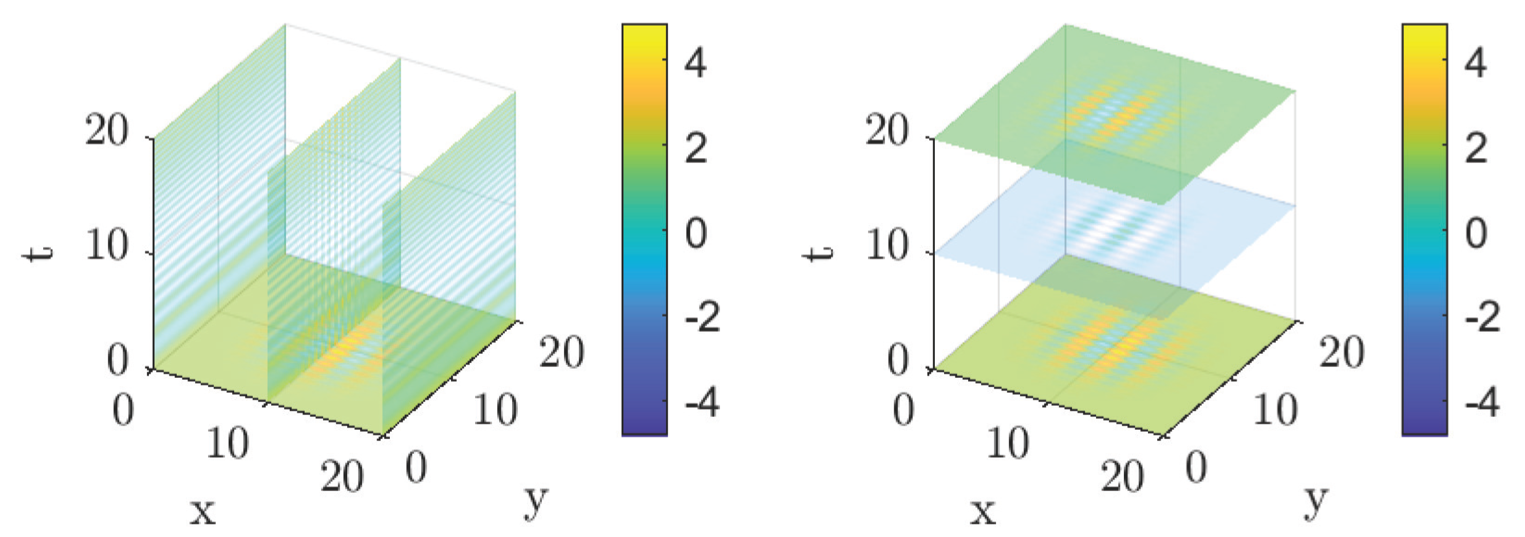
Figure 2.
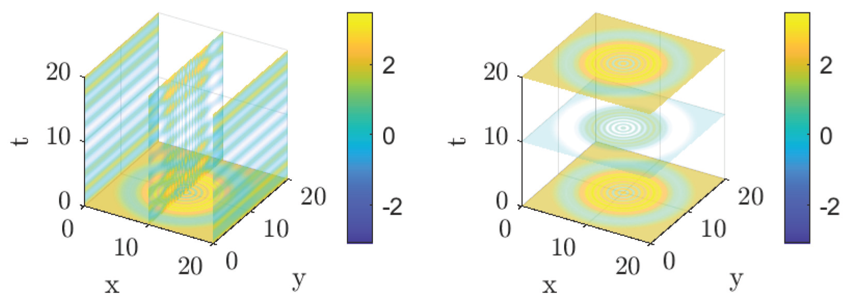
Example 1. (Left panel): 3D signal evolution in the second space variable and time. (Right panel): 3D signal evolution in space at different time stamps.
In Figure 2, the left panel presents a three-dimensional visualization of the signal, with the x and y axes corresponding to spatial coordinates and the z axis representing signal intensity. The color gradient encodes variations in amplitude across space and time. The right panel illustrates the temporal evolution of the signal at multiple spatial positions, capturing how the signal propagates and changes over time across the spatial domain.
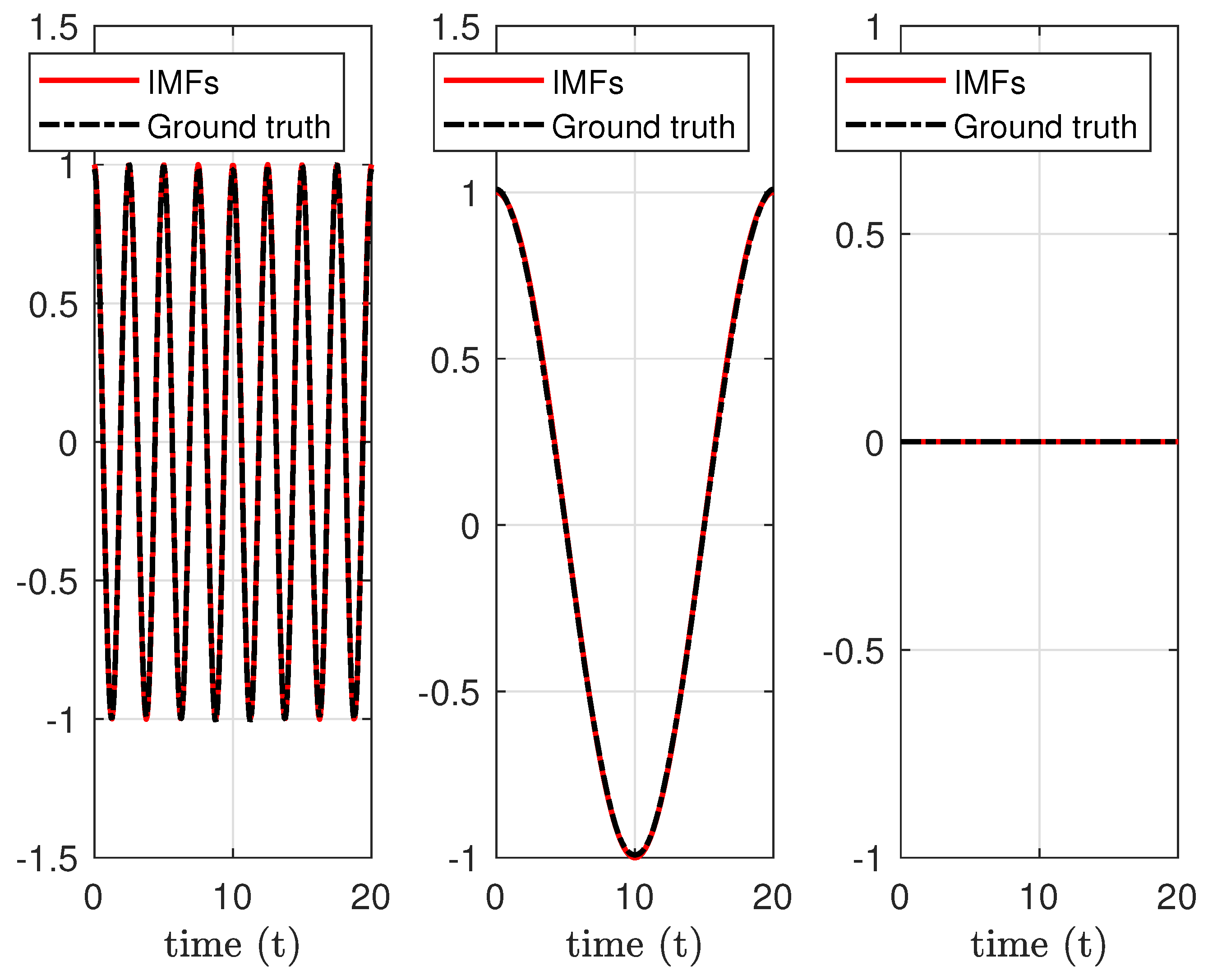
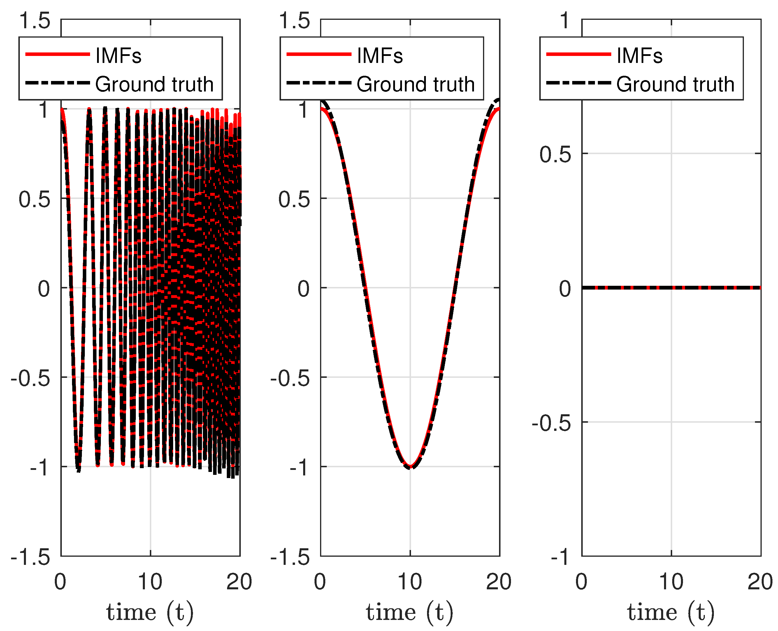
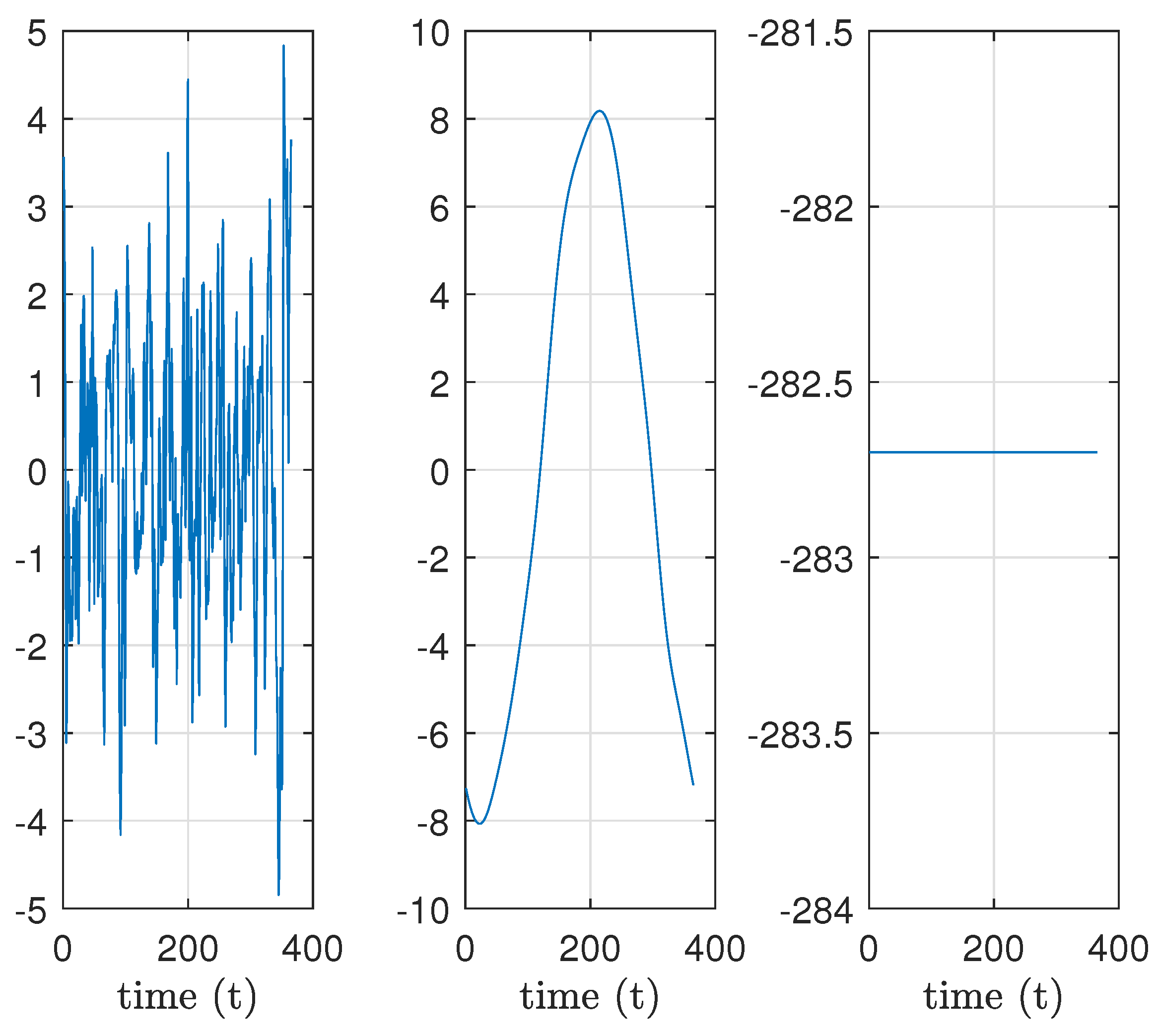
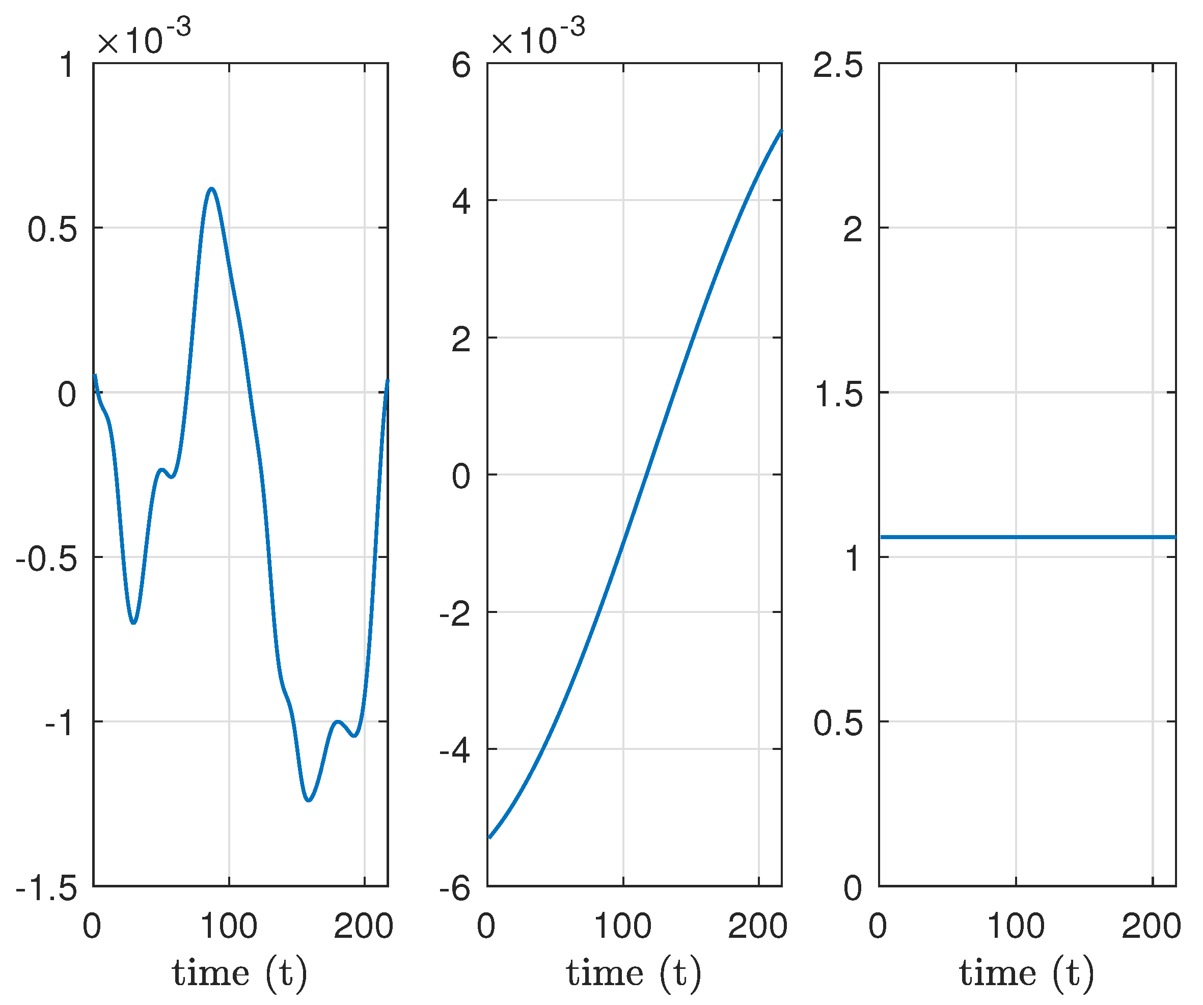
We apply MdMvFIF to decompose such signals into space and time IMFs. We plot in Figure 3 the time decomposition of the signal at the spatial position . The three plots represent different intrinsic mode functions (IMFs), with the red curves indicating the extracted signal components and the black curves representing the ground truth. The horizontal axis corresponds to time, while the vertical axis shows the signal amplitude.
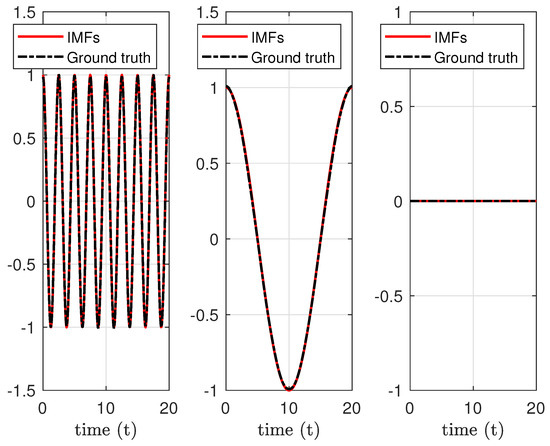
Figure 3.
Example 1. Time decomposition for data at position .
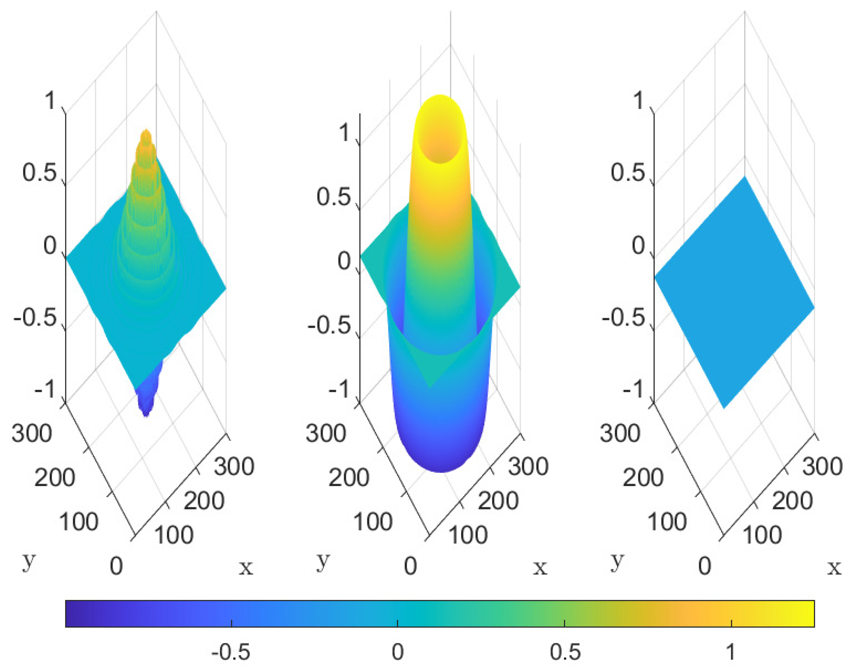
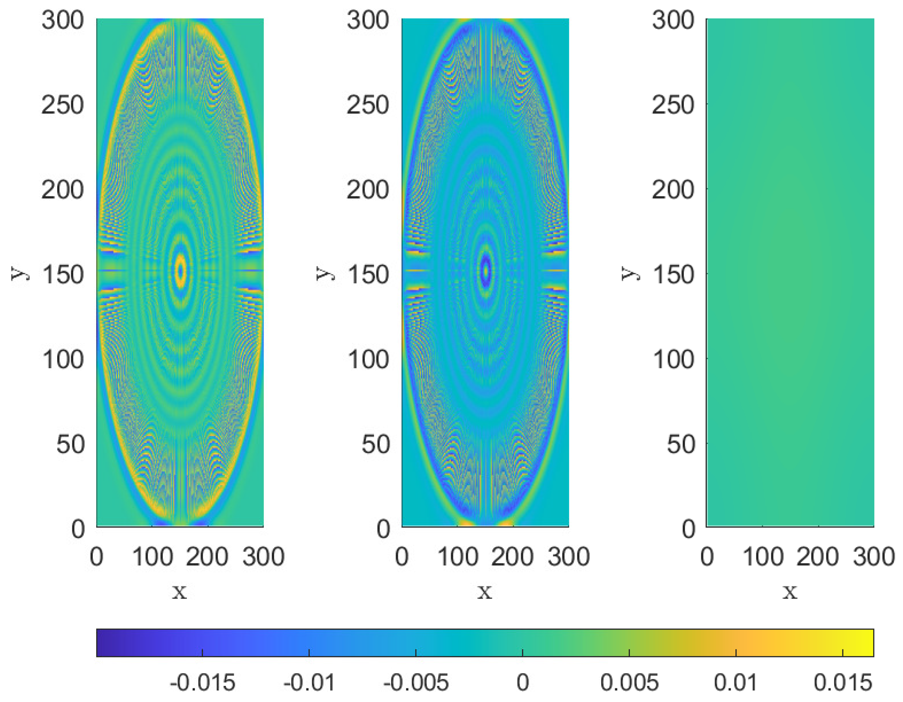
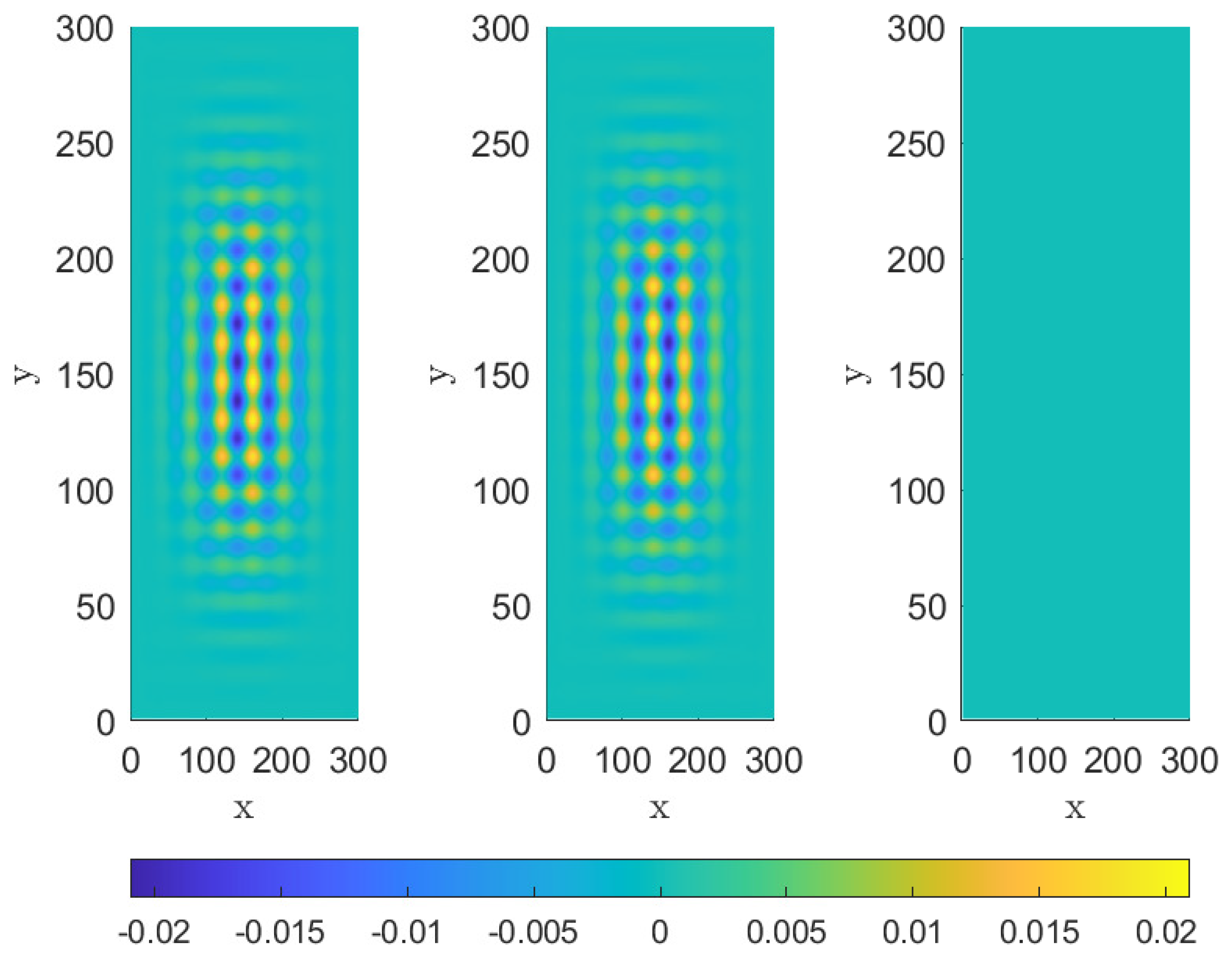
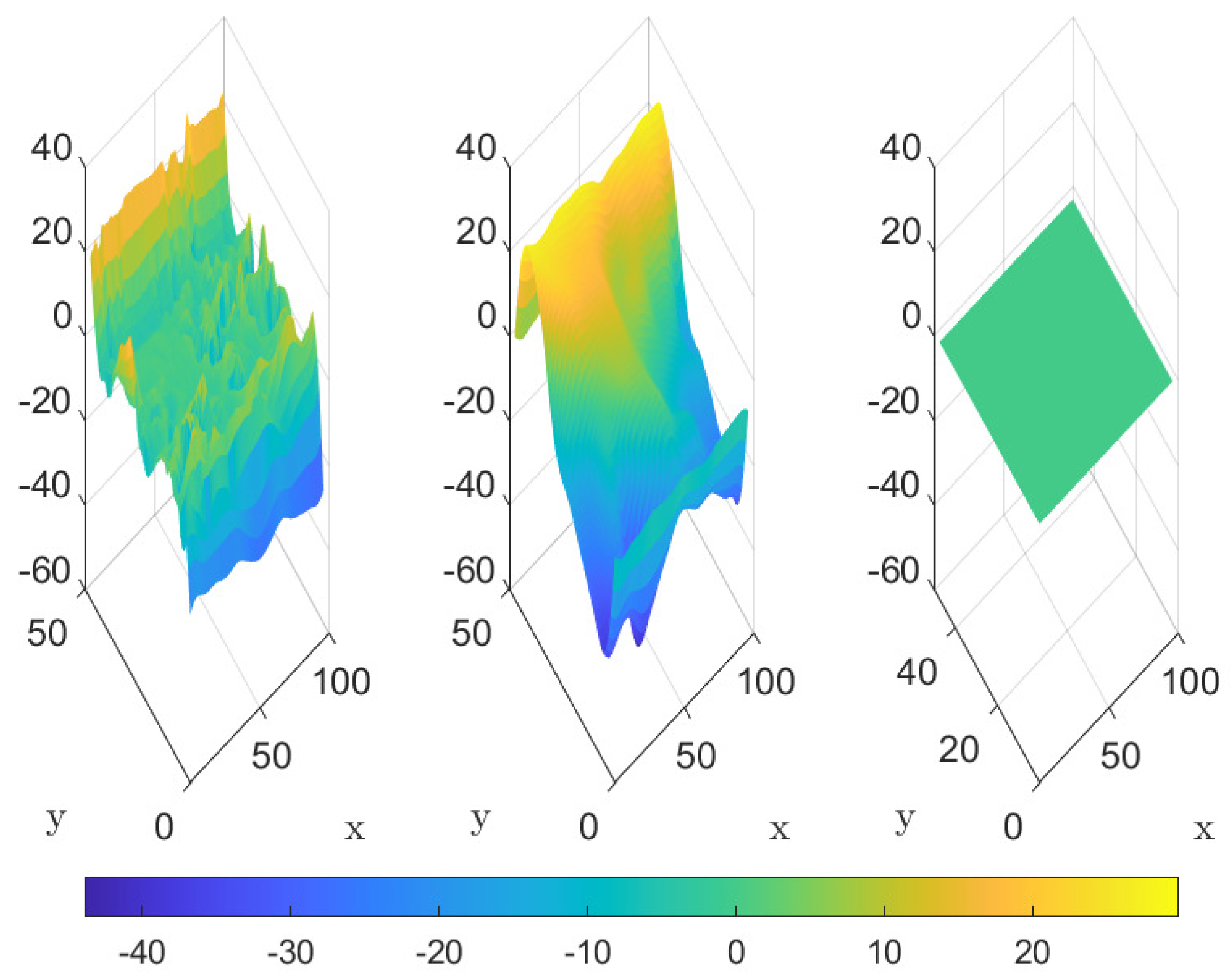
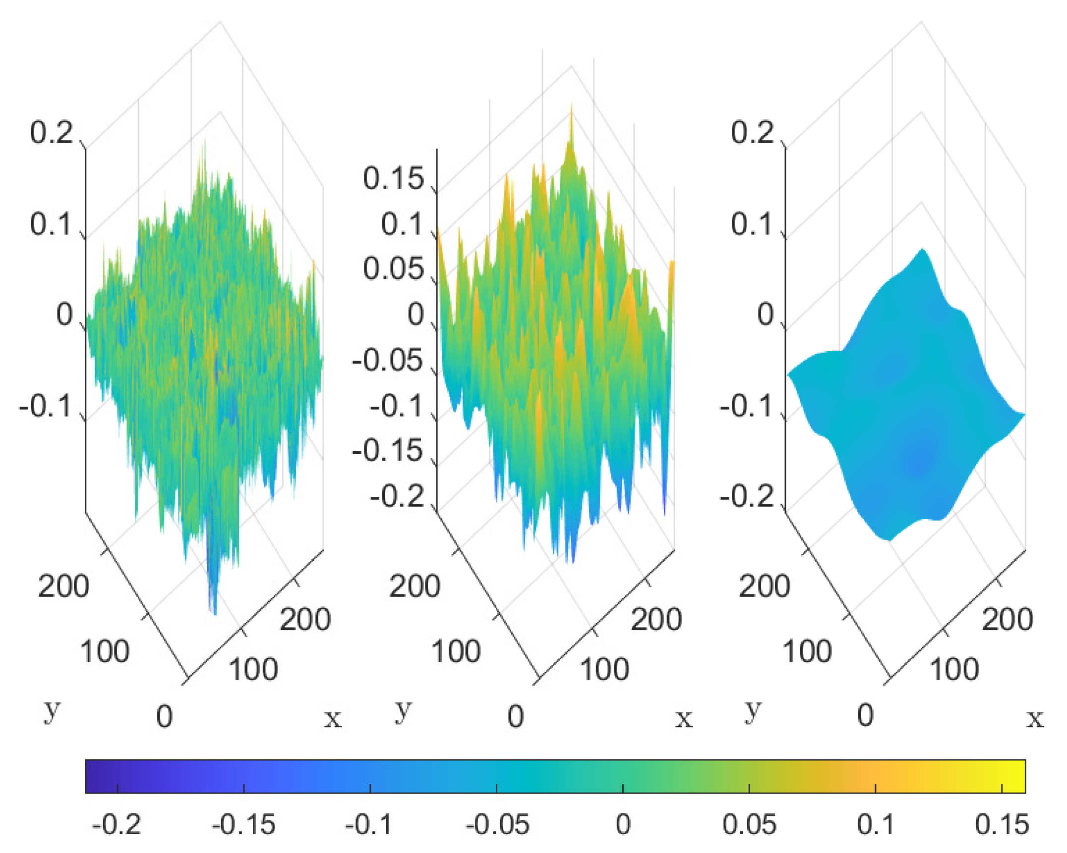
Figure 4 displays the spatial distribution of the first and second IMFs, along with the trend component of the signal produced with the proposed method. The x and x axes represent spatial coordinates, while the z axis reflects the signal amplitude. The color gradient indicates the intensity of each component across the spatial domain. Figure 5 illustrates the differences between the ground truth and the first and second IMF components produced by the MdMvFIF algorithm. The color map reflects the intensity of the differences, with x and y representing spatial positions and the color gradient showing the magnitude of variation. Since these differences are an order of magnitude of around , whereas the signal intensity is around 1, we can conclude that MdMvFIF can decompose this artificial signal with good accuracy.

Figure 4.
Example 1. From left to right, first, second IMF and trend over space.

Figure 5.
Example 1. Differences between the ground truth and the first and second IMF and trend produced over space by MdMvFIF algorithm, respectively.
To empirically verify the MdMvFIF algorithm’s complexity, we ran a series of tests on this example considering grids of increasing size. The CPU times and the values of the constant C in the expression time are reported in Table 1. The results confirm the expected trend, with . All tests were performed using MATLAB R2023b 64 bit on a standard laptop equipped with an 11th Gen Intel(R) Core(TM) i7-1185G7 processor running at 3.00 GHz using 16.0 GB of RAM.

Table 1.
CPU times and estimated constants C for various grid configurations.
3.2. Second Artificial Example
In this second example, we have a signal containing two non-stationary frequencies active in space and two non-stationary frequencies active in time. The data are shown in Figure 6 and Figure 7. Figure 6 illustrates the signal at time on a 2D spatial grid, where the x and y axes represent spatial positions. The color gradient, ranging from blue to yellow, encodes signal intensity at each point. The right panel shows the time evolution of the signal at the spatial location , with the horizontal axis representing time and the vertical axis indicating signal intensity. The color scale reflects variations in amplitude over time. Figure 7 presents a 3D visualization of the signal’s evolution over space and time, with the x and y axes representing spatial positions and the z axis corresponding to signal intensity. The color gradient reflects variations in intensity. The right panel shows a 3D representation of the signal evolution at different time points, with the same spatial axes and color gradient indicating changes in intensity.

Figure 6.
Example 2. (Left panel): Signal at time . (Right panel): Time evolution for position .
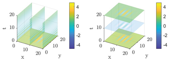
Figure 7.
Example 2. (Left panel): 3D signal evolution in the second space variable and time. (Right panel): 3D signal evolution in space at different time stamps.
We apply MdMvFIF to decompose such signals into space and time IMFs. We plot the results in Figure 8 and Figure 9. In Figure 10, we report the differences between the ground truth space components and the IMFs produced with the proposed method. Also in this second example, even though the signals are non-stationary both in time and space, the proposed algorithm can separate with a good level of accuracy the oscillations contained both in space and time.
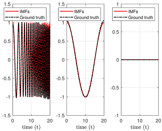
Figure 8.
Example 2. Time decomposition for data at position .
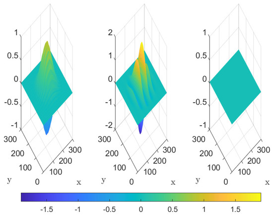
Figure 9.
Example 2. From left to right, first, second IMF and trend over space.

Figure 10.
Example 2. Differences between the ground truth and the first and second IMF and trend produced over space by the MdMvFIF algorithm, respectively.
Figure 8 illustrates the time decomposition of the signal at the spatial position . The three panels correspond to different intrinsic mode functions (IMFs), where the red lines represent the decomposed signal components and the black lines show the ground truth. The horizontal axis represents time and the vertical axis indicates signal amplitude. Figure 9 shows the spatial distribution of the first and second intrinsic mode functions (IMFs) and the trend component. The x and y axes represent spatial positions, and the z axis indicates signal amplitude, with the color gradient reflecting signal intensity.
Figure 10 displays the differences between the ground truth and the first two IMF components obtained with the MdMvFIF algorithm. The color map shows the intensity of these differences across the spatial domain, with the x and y axes representing spatial positions. Since these differences, like in the first artificial example, are an order of magnitude of around , whereas the signal intensity is around 1, we can conclude that MdMvFIF can also decompose this second artificial signal with good accuracy.
3.3. Earth’s Air Temperature
We now consider the first real-life signal: the Earth’s air temperature measured in kelvin on a global grid at an altitude of 2 m from the surface of our planet. This dataset is made available through the US National Center for Environmental Prediction (NCEP)/US National Center for Atmospheric Research (NCAR) Reanalysis project (the original NCEP Reanalysis data has been provided by the NOAA/OAR/ESRL PSD, Boulder, Colorado, USA http://www.esrl.noaa.gov/psd/ (accessed on 28 March 2025) and have been edited by the Climatic Research Unit, University of East Anglia https://crudata.uea.ac.uk/cru/data/ncep/ (accessed on 28 March 2025). This project aimed to produce a 40-year record of global analyses of atmospheric fields in support of the needs of the research and climate monitoring communities. The dataset is obtained through the NCEP Global Data Assimilation System (GDAS). In particular, they used global rawinsonde from the NCEP Global Telecommunications System (GTS) data with upper-air observations collected using pibals (ceiling balloons) and aircraft data and raobs (https://www.raob.com/) (accessed on 28 March 2025) from national archives in various countries; comprehensive Ocean-Atmosphere Data Set (COADS) (COADS is a joint project of NOAA/ERL, NCAR, NCDC, and many other organizations and countries) based on data collected using ships, fixed buoys, drifting buoys, pack-ice buoys, near-surface data from ocean station reports, and other data; aircraft data available from the NCEP GTS and other sources; surface land synoptic data made available from Air Force or NCEP sources; satellite sounder data obtained from several sources; Special Sensing Microwave/Imager (SSM/I) data; and satellite cloud drift winds based on the USA National Meteorological Center (NMC) tapes and from the USA Geostationary Meteorological Satellite (GMS) cloud drift winds. For more details on the project, we refer the interested reader to [46].
In this work, we consider the temperatures measured daily from 1 January 2022 to 31 December 2022 (Data are available at https://crudata.uea.ac.uk/cru/data/ncep/qs_eurasia/daily/sflux/air.2m/ (accessed on 28 March 2025) ). A sample of the data, the spatial distribution of air temperature on 10 April 2022, at a 2-m altitude, is displayed in Figure 11. In the left panel, the x and y axes represent spatial coordinates, and the color gradient (from blue to yellow) indicates temperature values in kelvin. The right panel displays the time evolution of air temperature at the spatial position , with the horizontal axis representing time and the vertical axis showing temperature values. The color scale reflects variations in temperature amplitude.
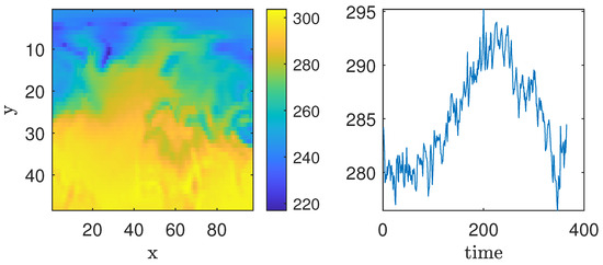
Figure 11.
Example 3. (Left panel): air temperature measured on 10 April 2022. (Right panel): Time evolution for position .
The data are stored as 3D tensors of dimension .
We apply MdMvFIF to decompose such signals into space and time IMFs. We plot the results in Figure 12 and Figure 13. From these results, it is possible to see how well MdMvFIF separates high frequencies, low frequencies, and trends both in space and time variations.

Figure 12.
Example 3. Decomposition over space of the data into two IMFs plus a trend.
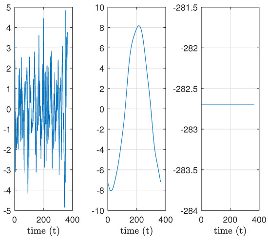
Figure 13.
Example 3. Time decomposition for data at position .
3.4. Thermal Imagery from Composite Material
An infrared camera recorded the thermal evolution on the back surface of a carbon-fiber-reinforced plastic (CFRP) material for approximately 17 seconds at a sampling rate of 120 frames per second (data are publicly available at https://data.mendeley.com/datasets/v4knrwgj9y/2 (accessed on 28 March 2025). For this test, we used the dataset CFRP-006_facq-120Hz_s-Back_Img-2000).
The thermal data acquisition spanned the phases before the application of a heat pulse, during the heat pulse, and during the cooling period. CFRP is a composite material composed of a synthetic resin matrix reinforced with embedded carbon fibers [47]. This experiment focused on the back face of the CFRP specimen to analyze deeper defect depths. The heat pulse was generated using two FX60 BALCAR photographic flashes, each delivering 6.2 kJ of energy in a 2 ms pulse. The flashes were positioned at a 45° angle to the sample surface, with their pulses aligned to the center of the sample. Thermal imaging was performed with a FLIR X6900 infrared camera equipped with an InSb CCD sensor matrix. The camera captured data at a resolution of 512 × 512 pixels with 14-bit intensity resolution and operated within a spectral range of 3.0 to 5.0 µm. The camera was positioned 1.0 m from the sample at a 90° angle to its surface. The sample’s emissivity was set to 0.98, and the flashes were placed 0.5 m from the sample to ensure efficient heat delivery. This setup ensured precise and repeatable data acquisition for thermal simulations, defect detection, and subsurface characterization of the back surface of the CFRP specimen.
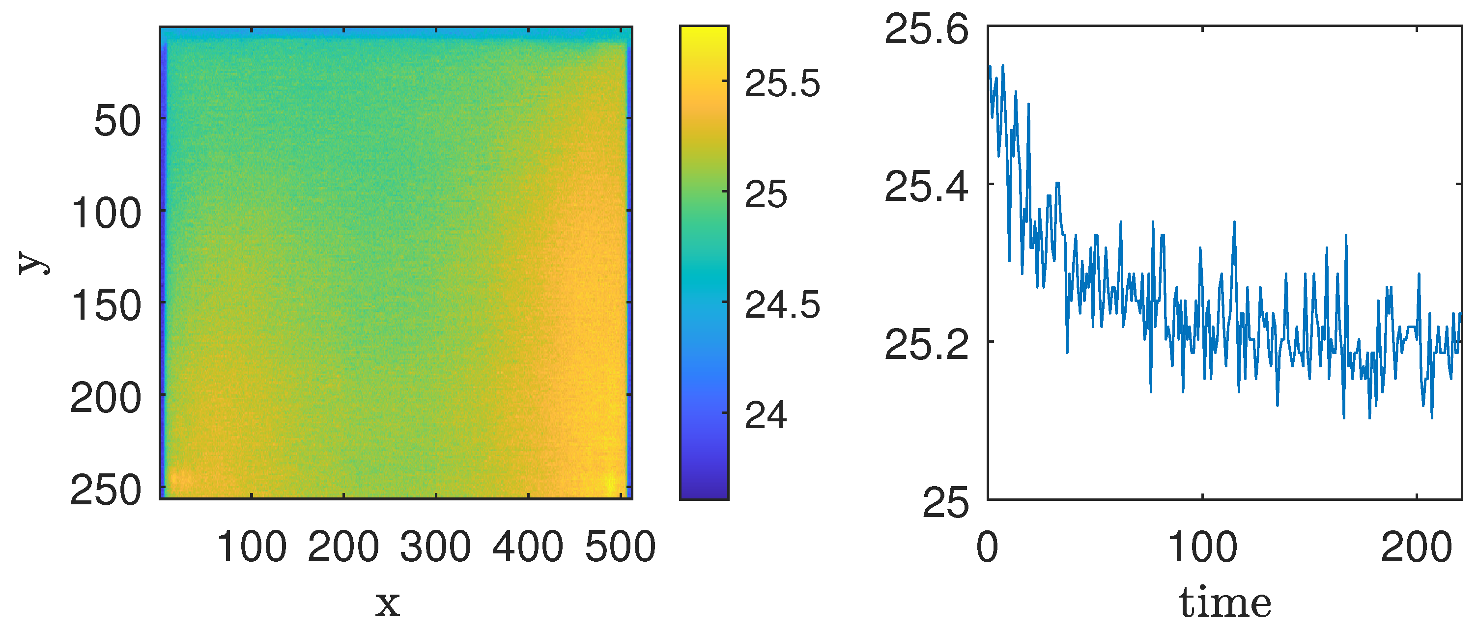
A sample of the data is shown in Figure 14. The left panel presents a spatial sample of the temperature on the material’s surface, with the x and y axes representing spatial coordinates, and the color scale indicating the temperature values. The right panel illustrates the time evolution of the temperature at the spatial position , with the horizontal axis representing time and the vertical axis showing temperature amplitude. The data are stored as 3D tensors of dimension . We apply MdMvFIF to decompose such signals into space and time IMFs. We plot the results in Figure 15 and Figure 16.

Figure 14.
Example 4. (Left panel): sample of the superficial heat of the CFRP material, frame 100. (Right panel): sample of the time evolution for position .
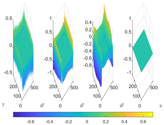
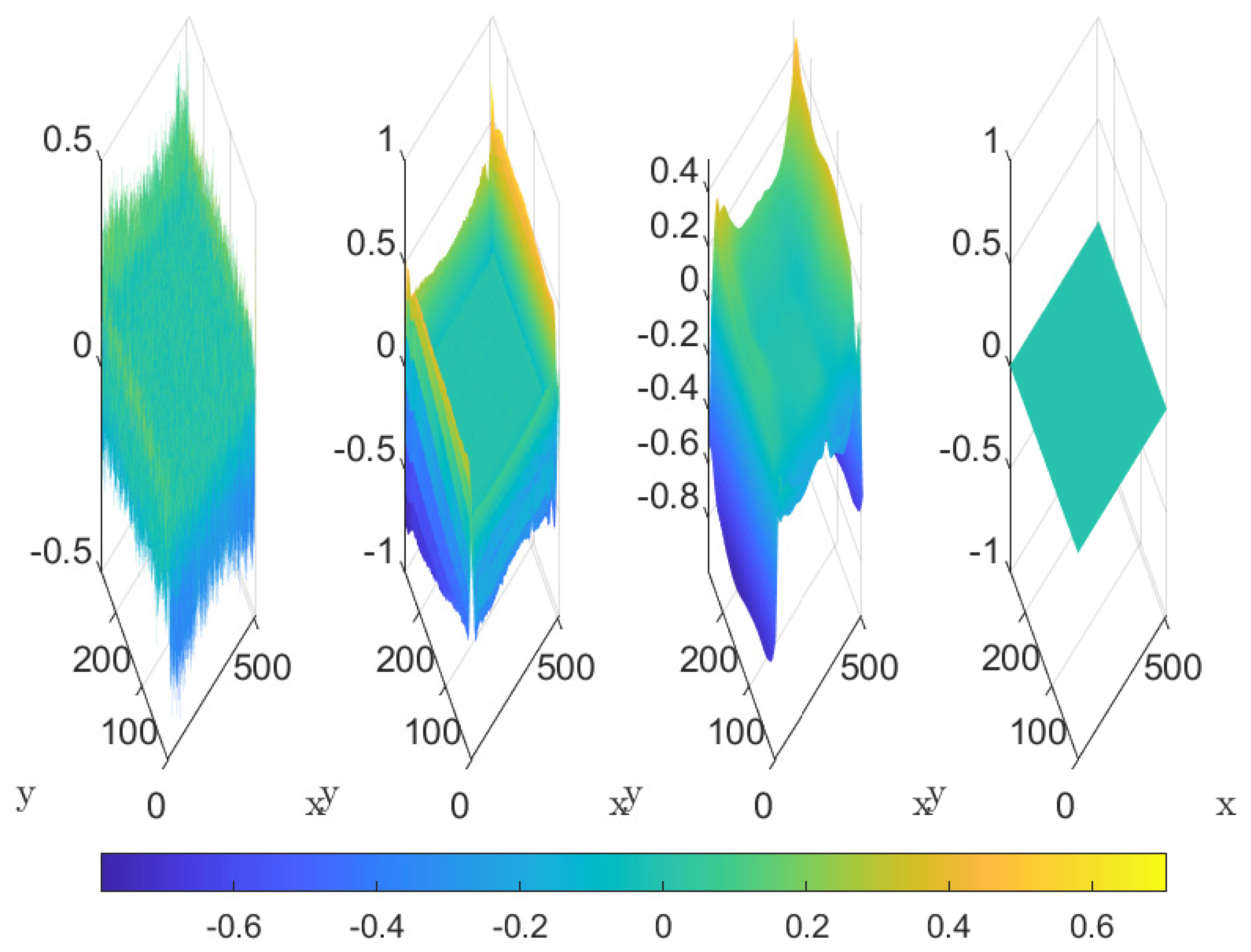
Figure 15.
Example 4. Decomposition over space of the data into three IMFs plus a trend.

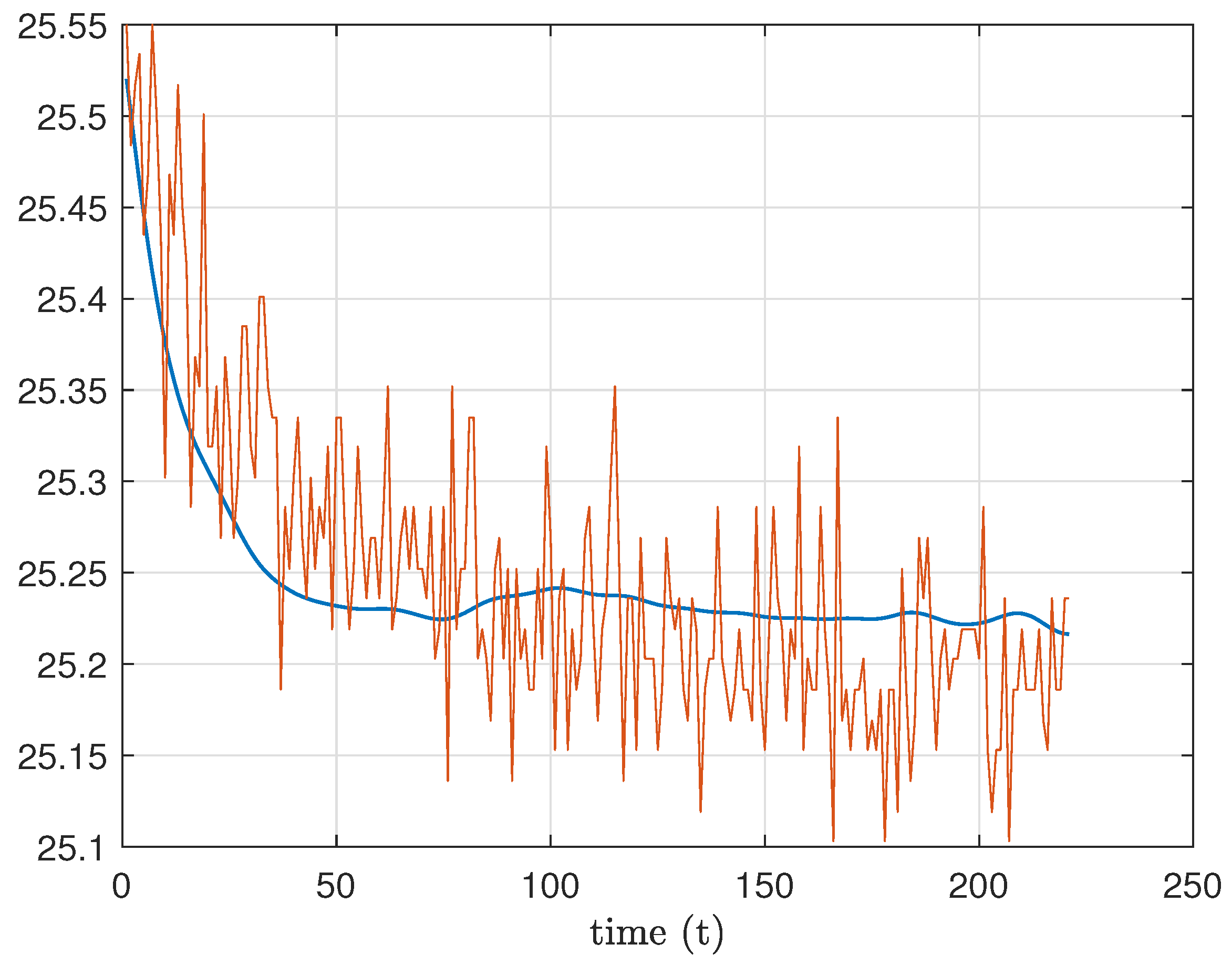
Figure 16.
Example 4. Time decomposition for data at position . In red the original signal, in blue the trend in time computed via MdMvFIF.
In this case, MdMvFIF allows us to identify in an adaptive way the trend both in the spatial and time data. In applications, the trend could be the useful information we want to preserve or the disturbance we may want to remove. For instance, in [38], the authors applied FIF2 to remove the trend in space and MvFIF to remove the high-frequency oscillations, preserving only the trend in time. With MdMvFIF, it will be possible to do it in a single shot.
3.5. Plasma Turbulence Simulations
The dataset used in this example was produced by a high-resolution numerical simulation of plasma turbulence, employing a fluid Hall-magnetohydrodynamic model (HMHD) of decaying plasma turbulence. Its evolution into fully developed turbulence, as well as its statistical properties have been thoroughly characterized in [48].
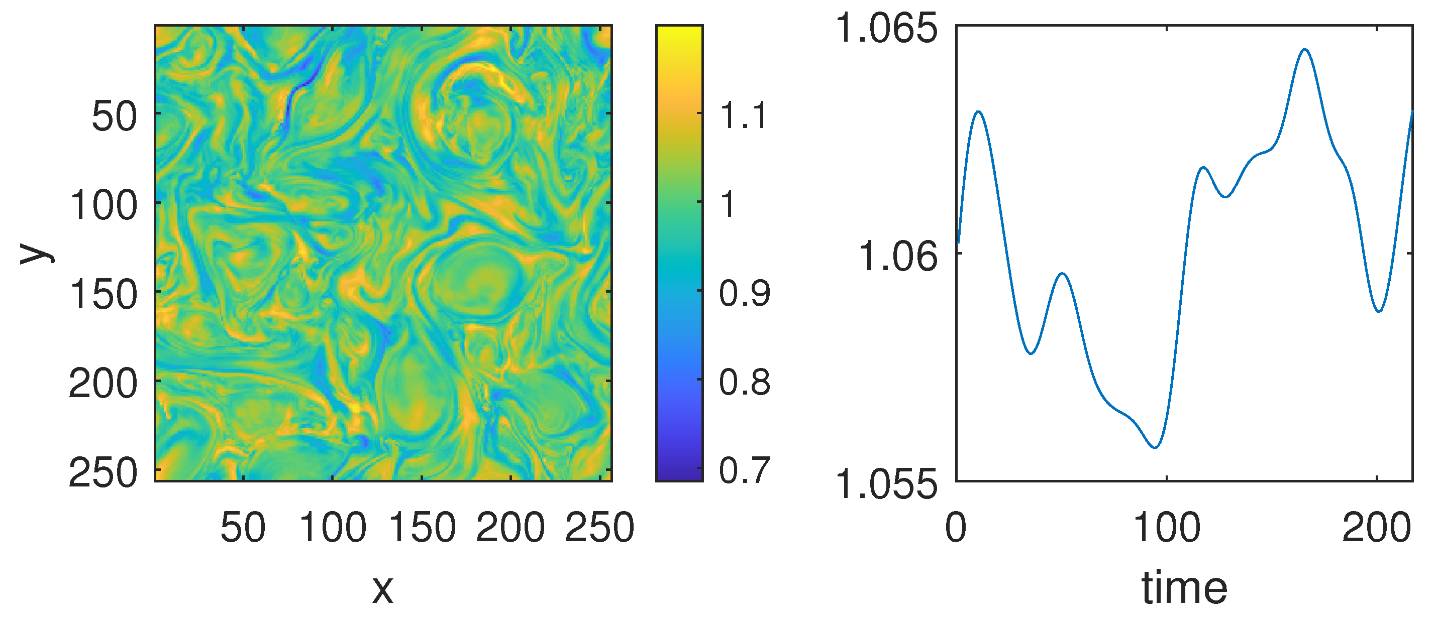
In this example, we consider the plasma density studied in [48]. For the purpose of this work, the original datacube of size was subsampled in space to and in time we considered the first 256 values from the original 1001, producing a 3D tensor of dimension . A sample of the data is shown in Figure 17. In the left panel, the x and y axes represent spatial positions, with the color scale indicating plasma density. The right panel displays the time evolution of plasma density at the spatial position , showing the variation of density over time. We apply MdMvFIF to decompose such signals into space and time IMFs. We plot the results in Figure 18 and Figure 19.
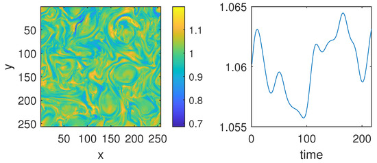
Figure 17.
Example 5. (Left panel): sample of the plasma density HMHD simulation at . (Right panel): sample of the time evolution for the plasma density at pixel .

Figure 18.
Example 5. Decomposition over space of the data into two IMFs plus a trend.
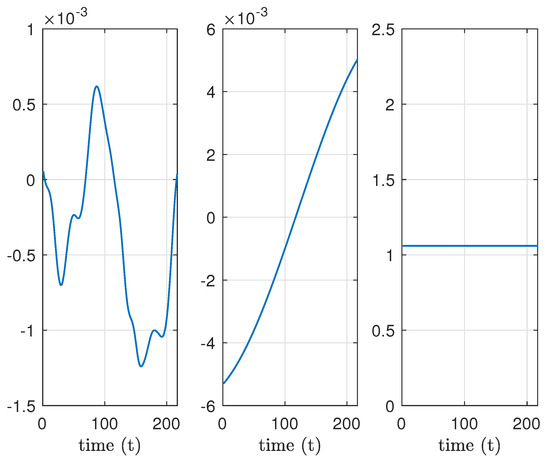
Figure 19.
Example 5. Time decomposition for data at position .
We observe that the oscillations extracted in time, Figure 19, differ slightly from the one present in time in the original data; refer to the right panel in Figure 17. This is because in the simulated data, space and time variations are tangled. This is an example of a real-life signal that requires the handling of time as a different variable from space and not as an extra spatial dimension as it is performed in the fast and adaptive empirical mode decomposition for multidimensional, multivariate signals (FA-MVEMD) [35], the fast empirical mode decomposition method for multidimensional signals based on serialization (Serial-EMD) [36], and the ST_FIF proposed in this paper.
4. Conclusions
In this work, we introduced the Multidimensional and Multivariate Fast Iterative Filtering (MdMvFIF) method and the Space Time Fast Iterative Filtering (ST_FIF), which are extensions of the Fast Iterative Filtering (FIF) algorithm designed to decompose complex signals that vary both in space and time. The MdMvFIF overcomes several limitations present in previous signal decomposition methods, such as the separation of time and space variations and the inability to independently filter different frequency ranges in space and time. The second one is an accelerated version of the first, but it has two important limitations: it does not allow to independently filter different frequency ranges in space and time, which is a fundamental feature in applications, and it requires the data to have separated spatial and time variations, which is usually not true in real-life signals. For these reasons, in the rest of the work, we focused on testing only the first proposed algorithm.
We demonstrated via several examples that the MdMvFIF method can be applied to high-dimensional and multivariate datasets, handling not only multidimensional signals but also signals that evolve over time. By iterating the filtering process first in space and then in time, the MdMvFIF method effectively isolates Intrinsic Mode Functions (IMFs) from complex data, making it a valid tool for the study of many real-world datasets. We presented several numerical examples, including synthetic signals and real-life data, to show the versatility and robustness of the approach.
In particular, the MdMvFIF algorithm provides a powerful tool for signal analysis in applications where the interplay between spatial and temporal variations is complex and intertwined. Future work will explore further optimization of the algorithm, including strategies for speeding up calculations preserving its ability to independently filter different frequency ranges in space and time, and its integration with machine learning techniques for feature extraction and analysis.
In conclusion, the MdMvFIF technique expands the capabilities of signal decomposition, offering a non-linear, adaptive, and efficient approach for analyzing multidimensional and multivariate signals that vary over both space and time. This makes it a promising method for a wide range of applications, like in engineering, physics, economics, medicine, and more general signal processing tasks.
As with other decomposition methods, MdMvFIF is sensitive to boundary effects. In this work, ideal boundary conditions were assumed in order to focus on the development and evaluation of the method itself. Addressing boundary treatment in a more robust and systematic way will be an important direction for future work.
Another potential limitation lies in the handling of mixed space-time modes, which may not be fully resolved due to the intrinsic structure of the algorithm. While this issue does not affect the artificial examples - where spatial and temporal variations were designed to be separable—it remains an open question when dealing with real - world data, where no ground truth is available. Investigating the behavior of the algorithm in such cases will be the focus of future research.
Finally, the computation of the filter support plays a crucial role in the performance of this class of methods. As discussed in this work, its optimal definition in higher dimensions is still an open problem, and we plan to address this issue in the future.
Author Contributions
Conceptualization, R.C., A.C., E.P. and H.Z.; methodology, R.C., A.C., E.P. and H.Z.; software, R.C., A.C., E.P. and H.Z.; validation, R.C., A.C., E.P. and H.Z.; formal analysis, R.C., A.C., E.P. and H.Z.; investigation, R.C., A.C., E.P. and H.Z.; resources, R.C., A.C., E.P. and H.Z.; data curation, R.C., A.C., E.P. and H.Z.; writing—original draft preparation, R.C., A.C., E.P. and H.Z.; writing—review and editing, R.C., A.C., E.P., and H.Z.; visualization, R.C., A.C., E.P. and H.Z.; supervision, R.C., A.C., E.P. and H.Z.; project administration, R.C., A.C., E.P. and H.Z.; funding acquisition, R.C., A.C., E.P. and H.Z. All authors have read and agreed to the published version of the manuscript.
Funding
A.C., E.P., and R.C. are members of the Gruppo Nazionale Calcolo Scientifico-Istituto Nazionale di Alta Matematica (GNCS-INdAM). The research of H.Z. is partially funded by NSF grant number DMS-2307465. The research of A.C. and R.C. were partially funded through the GNCS-INdAM Project, grant numbers CUP E53C22001930001, and CUP E53C23001670001. A.C. and E.P. were funded by the Italian Ministry of the University and Research and the European Union through the “Next Generation EU”, Mission 4, Component 1, under the PRIN PNRR 2022 grant number CUP E53D23018040001 ERC field PE1 project P2022XME5P titled “Circular Economy from the Mathematics for Signal Processing prospective”.
Data Availability Statement
Codes and examples available at www.cicone.com.
Conflicts of Interest
The authors declare no conflicts of interest. The funders had no role in the design of the study; in the collection, analyses, or interpretation of data; in the writing of the manuscript; or in the decision to publish the results.
References
- Ghobadi, H.; Spogli, L.; Alfonsi, L.; Cesaroni, C.; Cicone, A.; Linty, N.; Romano, V.; Cafaro, M. Disentangling ionospheric refraction and diffraction effects in GNSS raw phase through fast iterative filtering technique. GPS Solut. 2020, 24, 85. [Google Scholar] [CrossRef]
- Huang, N.E.; Shen, Z.; Long, S.R. A new view of nonlinear water waves: The Hilbert spectrum. Annu. Rev. Fluid Mech. 1999, 31, 417–457. [Google Scholar] [CrossRef]
- Moridian, P.; Shoeibi, A.; Khodatars, M.; Jafari, M.; Pachori, R.B.; Khadem, A.; Alizadehsani, R.; Ling, S.H. Automatic diagnosis of sleep apnea from biomedical signals using artificial intelligence techniques: Methods, challenges, and future works. Wiley Interdiscip. Rev. Data Min. Knowl. Discov. 2022, 12, e1478. [Google Scholar] [CrossRef]
- Terradas, J.; Oliver, R.; Ballester, J.L. Application of statistical techniques to the analysis of solar coronal oscillations. Astrophys. J. 2004, 614, 435. [Google Scholar] [CrossRef]
- Abdelouahad, A.A.; El Hassouni, M.; Cherifi, H.; Aboutajdine, D. Reduced reference image quality assessment based on statistics in empirical mode decomposition domain. Signal Image Video Process. 2014, 8, 1663–1680. [Google Scholar] [CrossRef]
- Li, X.; Su, J.; Yang, L. Building detection in SAR images based on bi-dimensional empirical mode decomposition algorithm. IEEE Geosci. Remote Sens. Lett. 2019, 17, 641–645. [Google Scholar] [CrossRef]
- Xia, Y.; Zhang, B.; Pei, W.; Mandic, D.P. Bidimensional multivariate empirical mode decomposition with applications in multi-scale image fusion. IEEE Access 2019, 7, 114261–114270. [Google Scholar] [CrossRef]
- Pathak, D.; Kashyap, R.; Rahamatkar, S. A study of deep learning approach for the classification of Electroencephalogram (EEG) brain signals. In Artificial Intelligence and Machine Learning for EDGE Computing; Academic Press: Cambridge, MA, USA, 2022; pp. 133–144. [Google Scholar]
- Yang, L.; Zhai, Y.; Li, Z. Deep learning for online AC false data injection attack detection in smart grids: An approach using LSTM-autoencoder. J. Netw. Comput. Appl. 2021, 193, 103178. [Google Scholar] [CrossRef]
- Zhang, Z.; Cui, P.; Zhu, W. Deep learning on graphs: A survey. IEEE Trans. Knowl. Data Eng. 2020, 34, 249–270. [Google Scholar] [CrossRef]
- Battista, B.M.; Knapp, C.; McGee, T.; Goebel, V. Application of the empirical mode decomposition and Hilbert-Huang transform to seismic reflection data. Geophysics 2007, 72, H29–H37. [Google Scholar] [CrossRef]
- Baykut, S.; Akgül, T.; İnan, S.; Seyis, C. Observation and removal of daily quasi-periodic components in soil radon data. Radiat. Meas. 2010, 45, 872–879. [Google Scholar] [CrossRef]
- Roberts, P.H.; Yu, Z.J.; Russell, C.T. On the 60-year signal from the core. Geophys. Astrophys. Fluid Dyn. 2007, 101, 11–35. [Google Scholar] [CrossRef]
- Bazzi, A.; Slock, D.T.M.; Meilhac, L. Efficient Maximum Likelihood Joint Estimation of Angles and Times of Arrival of Multiple Paths. In Proceedings of the 2015 IEEE Globecom Workshops (GC Wkshps), San Diego, CA, USA, 6–10 December 2015; pp. 1–7. [Google Scholar]
- Chen, Y.; Zhang, H.; Liu, Y. Application of empirical mode decomposition in communication signal denoising. J. Commun. 2014, 9, 519–525. [Google Scholar]
- Proakis, J.G.; Salehi, M. Digital Communications; McGraw-Hill: New York, NY, USA, 2007. [Google Scholar]
- Cicone, A.; Liu, J.; Zhou, H. Adaptive local iterative filtering for signal decomposition and instantaneous frequency analysis. Appl. Comput. Harmon. Anal. 2016, 41, 384–411. [Google Scholar] [CrossRef]
- Yang, A.C.; Peng, C.K.; Huang, N.E. Causal decomposition in the mutual causation system. Nat. Commun. 2018, 9, 3378. [Google Scholar] [CrossRef]
- Costa, M.; Goldberger, A.L.; Peng, C.K. Broken asymmetry of the human heartbeat: Loss of time irreversibility in aging and disease. Phys. Rev. Lett. 2005, 95, 198102. [Google Scholar] [CrossRef]
- Wang, C.; Choi, H.J.; Kim, S.; Desai, A.; Lee, N.; Kim, D.; Bae, Y.; Lee, K. Deconvolution of subcellular protrusion heterogeneity and the underlying actin regulator dynamics from live cell imaging. Nat. Commun. 2018, 9, 04030. [Google Scholar] [CrossRef]
- Hillier, A.; Morton, R.J.; Erdélyi, R. A statistical study of transverse oscillations in a quiescent prominence. Astrophys. J. Lett. 2013, 779, L16. [Google Scholar] [CrossRef]
- Daubechies, I.; Lu, J.; Wu, H.T. Synchrosqueezed wavelet transforms: An empirical mode decomposition-like tool. Appl. Comput. Harmon. Anal. 2011, 30, 243–261. [Google Scholar] [CrossRef]
- Huang, N.E.; Shen, Z.; Long, S.R.; Wu, M.C.; Shih, H.H.; Zheng, Q.; Yen, N.-C.; Tung, C.C.; Liu, H.H. The empirical mode decomposition and the hilbert spectrum for nonlinear and non-stationary time series analysis. Proc. R. Soc. Lond. Ser. Math. Phys. Eng. Sci. 1998, 454, 903–995. [Google Scholar] [CrossRef]
- Hou, T.Y.; Shi, Z. Adaptive data analysis via sparse time-frequency representation. Adv. Adapt. Data Anal. 2011, 3, 1–28. [Google Scholar] [CrossRef]
- Yu, S.; Ma, J.; Osher, S. Geometric mode decomposition. Inverse Probl. Imaging 2018, 12, 831–852. [Google Scholar] [CrossRef]
- Bai, Y.; Xue, H.; Chen, J. Train Axlebox Bearing Fault Diagnosis Based on MSC-SGMD. Sensors 2023, 24, 254. [Google Scholar] [CrossRef]
- Pan, H.; Yang, Y.; Li, X.; Zheng, J.; Cheng, J. Symplectic geometry mode decomposition and its application to rotating machinery compound fault diagnosis. Mech. Syst. Signal Process. 2019, 114, 189–211. [Google Scholar] [CrossRef]
- Gilles, J. Empirical wavelet transform. IEEE Trans. Signal Process. 2013, 61, 3999–4010. [Google Scholar] [CrossRef]
- Dragomiretskiy, K.; Zosso, D. Variational mode decomposition. IEEE Trans. Signal Process. 2013, 62, 531–544. [Google Scholar] [CrossRef]
- Sun, Y.; Qian, D.; Zheng, J.; Liu, Y.; Liu, C. Seismic Signal Analysis Based on Variational Mode Decomposition and Hilbert Transform for Ground Intrusion Activity Classification. Sensors 2023, 23, 3674. [Google Scholar] [CrossRef]
- Lin, L.; Wang, Y.; Zhou, H. Iterative filtering as an alternative algorithm for empirical mode decomposition. Adv. Adapt. Data Anal. 2009, 1, 543–560. [Google Scholar] [CrossRef]
- Cicone, A.; Pellegrino, E. Multivariate Fast Iterative Filtering for the Decomposition of Nonstationary Signals. IEEE Trans. Signal Process. 2022, 70, 1521–1531. [Google Scholar] [CrossRef]
- Cicone, A.; Zhou, H. Multidimensional iterative filtering method for the decomposition of high-dimensional non-stationary signals. Numer. Math. Theory Methods Appl. 2017, 10, 278–298. [Google Scholar] [CrossRef]
- Sfarra, S.; Cicone, A.; Yousefi, B.; Perilli, S.; Robol, L.; Maldague, X.P.V. Maximizing the detection of thermal imprints in civil engineering composites via numerical and thermographic results pre-processed by a groundbreaking mathematical approach. Int. J. Therm. Sci. 2022, 177, 107553. [Google Scholar] [CrossRef]
- Thirumalaisamy, M.R.; Ansell, P.J. Fast and adaptive empirical mode decomposition for multidimensional, multivariate signals. IEEE Signal Process. Lett. 2018, 25, 1550–1554. [Google Scholar] [CrossRef]
- Zhang, J.; Feng, F.; Marti-Puig, P.; Caiafa, C.F.; Sun, Z.; Duan, F.; Solé-Casals, J. Serial-EMD: Fast empirical mode decomposition method for multi-dimensional signals based on serialization. Inf. Sci. 2021, 581, 215–232. [Google Scholar] [CrossRef]
- Papini, E.; Cicone, A.; Piersanti, M.; Franci, L.; Hellinger, P.; Landi, S.; Verdini, A. Multidimensional Iterative Filtering: A new approach for investigating plasma turbulence in numerical simulations. J. Plasma Phys. 2020, 86, 871860501. [Google Scholar] [CrossRef]
- Tshiangomba, R.K.; Russo, G.; Ding, Y.; Pellegrino, E.; Zhang, H.; Sfarra, S.; Cicone, A. Solar Loading Infrared Thermography Method for the Non-Invasive Inspection of Movable Art: The Contribution of Multivariate Fast Iterative Filtering and Multidimensional Fast Iterative Filtering for 2D Data Techniques. Infrared Phys. Technol. 2025, 147, 105770. [Google Scholar] [CrossRef]
- Stallone, A.; Cicone, A.; Materassi, M. New insights and best practices for the successful use of empirical mode decomposition, iterative filtering and derived algorithms. Sci. Rep. 2020, 10, 15161. [Google Scholar] [CrossRef]
- Chen, B.; Chen, X.; Chen, F.; Zhou, B.; Xiao, W.; Fu, W.; Li, G. Integrated early fault diagnosis method based on direct fast iterative filtering decomposition and effective weighted sparseness kurtosis to rolling bearings. Mech. Syst. Signal Process. 2022, 171, 108897. [Google Scholar] [CrossRef]
- Sharma, R.; Pachori, R.B.; Upadhyay, A. Automatic sleep stages classification based on iterative filtering of electroencephalogram signals. Neural Comput. Appl. 2017, 28, 2959–2978. [Google Scholar] [CrossRef]
- Spogli, L.; Sabbagh, D.; Perrone, L.; Scotto, C.; Cesaroni, C. Investigating the drivers of long-term trends in the upper atmosphere over Rome across four decades. J. Space Weather. Space Clim. 2025, 15, 8. [Google Scholar] [CrossRef]
- Zhou, P.; Chen, S.; He, Q.; Wang, D.; Peng, Z. Rotating machinery fault-induced vibration signal modulation effects: A review with mechanisms, extraction methods and applications for diagnosis. Mech. Syst. Signal Process. 2023, 200, 110489. [Google Scholar] [CrossRef]
- Cicone, A.; Zhou, H. Numerical analysis for iterative filtering with new efficient implementations based on FFT. Numer. Math. 2021, 147, 1–28. [Google Scholar] [CrossRef]
- Rilling, G.; Flandrin, P. One or two frequencies? The empirical mode decomposition answers. IEEE Trans. Signal Process. 2008, 56, 85–95. [Google Scholar] [CrossRef]
- Kalnay, E.; Kanamitsu, M.; Kistler, R.; Collins, W.; Deaven, D.; Gandin, L.; Iredell, M.; Saha, S.; White, G.; Woollen, J.; et al. The ncep/ncar 40-year reanalysis project. Bull. Am. Meteorol. Soc. 1996, 77, 437–471. [Google Scholar] [CrossRef]
- Erazo-Aux, J.; Loaiza-Correa, H.; Restrepo-Giron, A.D.; Ibarra-Castanedo, C.; Maldague, X. Thermal imagery from composite material academic samples. Mendeley Data 2020, 32, 106313. [Google Scholar]
- Papini, E.; Cicone, A.; Franci, L.; Piersanti, M.; Landi, S.; Hellinger, P.; Verdini, A. Spacetime Hall-MHD Turbulence at Sub-ion Scales: Structures or Waves? Astrophys. J. Lett. 2021, 917, L12. [Google Scholar] [CrossRef]


Disclaimer/Publisher’s Note: The statements, opinions and data contained in all publications are solely those of the individual author(s) and contributor(s) and not of MDPI and/or the editor(s). MDPI and/or the editor(s) disclaim responsibility for any injury to people or property resulting from any ideas, methods, instructions or products referred to in the content. |
© 2025 by the authors. Licensee MDPI, Basel, Switzerland. This article is an open access article distributed under the terms and conditions of the Creative Commons Attribution (CC BY) license (https://creativecommons.org/licenses/by/4.0/).