Short-Term Predictions of Global Horizontal Irradiance Using Recurrent Neural Networks, Support Vector Regression, Gradient Boosting Random Forest and Advanced Stacking Ensemble Approaches

Abstract

In today’s world, where sustainable energy is essential for the planet’s survival, accurate solar energy forecasting is crucial. This study focused on predicting short-term Global Horizontal Irradiance (GHI) using minute-averaged data from the Southern African Universities Radiometric Network (SAURAN) at the Univen Radiometric Station in South Africa. Various techniques were evaluated for their predictive accuracy, including Recurrent Neural Networks (RNNs), Support Vector Regression (SVR), Gradient Boosting (GB), Random Forest (RF), Stacking Ensemble, and Double Nested Stacking (DNS). The results indicated that RNN performed the best in terms of mean absolute error (MAE) and root mean squared error (RMSE) among the machine learning models. However, Stacking Ensemble with XGBoost as the meta-model outperformed all individual models, improving accuracy by 67.06% in MAE and 22.28% in RMSE. DNS further enhanced accuracy, achieving a 93.05% reduction in MAE and an 88.54% reduction in RMSE compared to the best machine learning model, as well as a 78.89% decrease in MAE and an 85.27% decrease in RMSE compared to the best single stacking model. Furthermore, experimenting with the order of the DNS meta-model revealed that using RF as the first-level meta-model followed by XGBoost yielded the highest accuracy, showing a 47.39% decrease in MAE and a 61.35% decrease in RMSE compared to DNS with RF at both levels. These findings underscore advanced stacking techniques’ potential to improve GHI forecasting significantly.

1. Introduction

1.1. Overview

Renewable energy will play a crucial role in the future by providing sustainable, environmentally friendly alternatives to fossil fuels. It enhances energy security, fosters economic growth, and helps mitigate the impacts of climate change. Energy resources can be broadly categorised into fossil fuels, renewable energy, and nuclear energy. Among these, renewable energy stands out due to its ability to generate energy with significantly lower carbon emissions, making it a key strategy for reducing carbon footprints. Many countries are now prioritising renewable energy as a primary method to decrease emissions. Historically, fossil fuels have been the dominant energy source, but their extensive use—driven by rapid population growth and convenience—has resulted in severe environmental consequences. Research has highlighted these negative effects and reinforced the viability and sustainability of renewable energy [1].

Among the different types of renewable energy, solar energy is particularly noteworthy for its cleanliness and widespread availability. Solar energy, derived from the sun, is an abundant and virtually limitless free energy source. Despite its advantages, solar energy does face challenges, particularly the high costs associated with harvesting it. However, this issue is gradually being addressed as nations and corporations invest heavily in solar energy projects. These investments lead to technological advancements and a steady decline in operational costs over time [2].

1.2. Literature Review

S. Gbémou [3] conducted one such study, which compared machine learning models with a scaled persistence model in forecasting GHI. The study analysed the performance of artificial neural networks (ANNs), Gaussian process regression (GPR), SVR, and Long Short-Term Memory (LSTM) models. Two years’ worth of GHI data were used to train the models. Following the application of the coverage width-based criterion, dynamic mean absolute error (DMAE), and normalised root mean square error (nRMSE), the results showed that the machine learning models performed better than the scaled persistence model, with the SVR, LSTM, and GPR models being the top performers.

A recent study conducted in India by SVS Rajaprasad [4] focused on short-term forecasting of GHI using machine learning methods. The study proposed a new hybrid deep neural network-based (DNN) model that combined a convolutional neural network with bi-directional LSTM (CNN BiLSTM) and compared it with LSTM and BiLSTM as deep learning models. The study used one-minute interval GHI data for January 2023 to train and test these models. The proposed hybrid model outperformed LSTM and BiLSTM. This suggests that combining different machine learning methods can enhance the accuracy of GHI forecasting [4].

In a study conducted by Z. Yamani [5], it was noted that deep learning models, particularly LSTM, have been successful in forecasting tasks. However, the accuracy of the forecasting results depends not only on the robustness of the model but also on the amount of training data fed into the model. Most LSTM models have been found to require a relatively large amount of data. The study’s authors experimented with the accuracy of LSTM depending on the training data used. The study utilised three datasets of historic GHI from Saudi Arabia. The aim was to determine the minimum amount of data required for forecasting one hour. This was achieved by training the LSTM with five years of data and gradually reducing the amount of data fed into the model to compare the accuracy. Using nRMSE, the study found that LSTM can achieve excellent GHI forecasting accuracy with at least two years of training data.

In a recent study, researchers aimed to forecast the GHI, Diffuse Horizontal Irradiance (DNI), and Beam Normal Irradiance (BNI). They sought to predict hourly solar irradiation for different time horizons, including one hour and six hours ahead. The study utilised data from Odeillo, France, which exhibits high meteorological variability. The researchers trained the models using RF, Artificial Neural Networks (ANN), and Smart Persistence (SP) and assessed their performance using the Normalised Root Mean Square Error (NRMSE). The results indicated that RF accurately predicted GHI, DNI, and BNI compared to ANN and SP. Additionally, the study conducted seasonal analysis, revealing that winter and summer are the best seasons for forecasting, as opposed to spring and autumn. Furthermore, the predictability of the three components was compared, showing that GHI is less complex to predict compared to BNI and DNI, as the latter two are more sensitive to meteorological conditions [6].

In another recent study conducted in India by K. Naveen [7], researchers investigated solar radiation and focused on forecasting hourly GHI. The historical data used covered all climatic zones from 1995 to 2014. The study’s primary goal was to develop a high-performing model based on Gradient Boosting (GB) that also required less computational time. The GB model was benchmarked against a two-layer feed-forward neural network (FFN) and Auto-Regressive Integrated Moving Average (ARIMA). The results indicated that the GB model outperformed the FFN and displayed better accuracy than the ARIMA model, such as MSE and MAE. The developed model and its architecture are intended to have practical implications.

Stacking Ensemble models, similar to machine learning models, are used for forecasting in various domains. One of the most significant application areas for these models is in the field of renewable energy. However, there is a lack of research that has employed Stacking Ensemble methods for forecasting GHI.

One study implemented Stacking Ensemble methods in forecasting to improve the accuracy of solar irradiance prediction. They evaluated the efficacy of the Stacking Ensemble technique against single models like the Multi-Layer Perceptron (MLP), Bootstrap aggregating (Bagging) regressor, and Adaptive Boosting (AdaBoost) models. The same models were combined through Stacking Ensemble, and the resulting ensemble method was evaluated using determination coefficient, mean absolute error (MAE), and root mean squared error (RMSE). The researchers found that the Stacking Ensemble method outperformed all the single models, thus improving the prediction accuracy [8].

In a study by X. Guo [9], forecasting accuracy was investigated using the Stacking Ensemble principle. The study proposed using a single Stacking Ensemble model to predict PV power. This model was chosen for its ability to combine different principles and characteristics of various models to produce accurate predictions. Individual training was conducted for the models (XGBOOST, RF, CATBoost, LGBM) that would be stacked in the ensemble model to ensure a fair assessment of prediction accuracy. These models were combined using SVR for the second level and then compared with the Stacking Ensemble model. The data for training these models was collected from the Data Collection System (DCS) and included meteorological data. The prediction accuracy of power generation was considered in different weather settings, including rainy and sunny days. After combining these models and using RMSE to compare the results, it was found that XGBoost demonstrated superiority compared to each model. Furthermore, compared to the Stacking Ensemble, the RMSE of the Stacking Ensemble was 1.84% lower.

In a study by Zhou [10], a new ensemble model called Double Nested Stacking (DNS) was proposed for photovoltaic power forecasting. The DNS model used base models to generate predictions at the first level, which were then used as features to train higher-level meta-models. This resulted in a more sophisticated ensemble with enhanced predictive capabilities, aiming to improve accuracy. The proposed DNS model outperformed the traditional Stacking Ensemble model, built based on a gradient-boosting decision tree (GBDT), XGBoost, and SVR. The study used PV power station data from 2019 to 2023 and validated the effectiveness of the DNS model in improving forecasting accuracy.

1.3. Research Highlights and Contributions

The primary contribution of this study is a comparative analysis of the predictive capabilities of various machine learning and deep learning algorithms, as well as a Stacking Ensemble modelling framework for short-term forecasting of Global Horizontal Irradiance (GHI). This analysis utilises data from the Southern African Universities Radiometric Network (SAURAN) at the Univen Radiometric Station in South Africa.

The paper is organised as follows: Section 2 discusses the modelling approaches for GHI prediction, which include Recurrent Neural Networks (RNNs), Support Vector Regression (SVR), Gradient Boosting (GB), Random Forest (RF), Stacking Ensemble, and Double Nested Stacking (DNS). Section 3 presents empirical results highlighting the performance of each model, measured by mean absolute error (MAE) and Root Mean Squared Error (RMSE).

2. Models

Our study utilises GHI data from the SAURAN Univen radiometric station. The data are minute-averaged and consist of variables such as temperature, humidity, wind speed, cloud cover, etc. The data can be accessed through the following website: https://sauran.ac.za/, (accessed on 24 May 2024).

Figure 1 shows the Stacking Ensemble approach for short-term Global Horizontal Irradiance (GHI) predictions. The process involves preprocessing, training base models (RNN, SVR, RF, GB), generating predictions, training a meta-learner, and evaluating the final ensemble output. A detailed discussion of the methods is given as follows.

2.1. Recurrent Neural Networks

ANN models have been extensively studied to achieve human-like performance, particularly in pattern recognition. Among these, RNNs are ANNs that excel as a powerful tool for processing time series data. This is due to their inherent ability to capture temporal dependencies within sequential data. Unlike traditional feed-forward neural networks, RNNs have loops within their architecture, which allow them to maintain a memory of past inputs while processing new ones [11]. RNNs are defined as follows:

$$y_j(t+1)=\phi (\sum _{i=1}^{m+n}{w}_{ij}{z}_i\left(t\right))$$

(1)

$$z_i\left(t\right)=\left\{\begin{array}{cc}{y}_i\left(t\right)\hfill & \mathrm{if}(i\ge n)\hfill \\ u_{i-n}\hfill & \mathrm{if}(i>n),\hfill \end{array}\right.$$

(2)

where m stands for the proportion of inputs, and n for the hidden and output neurons, $\phi$ is the arbitrary differential component, generally a sigmoid function, and $y_j$ determines the output of the jth neuron and $w_{ij}$ the relationship between the ith and the jth neuron [12]. An RNN achieves its capability through recurrent neural connections. A fundamental equation for processing an input sequence $x=(x_1,x_2,\dots ,x_T)$ to determine the RNN hidden state $h_t$ is as follows:

$$h_t=\left\{\begin{array}{cc}0,\hfill & \mathrm{if}t=0\hfill \\ \Phi (h_{t-1},x_t),\hfill & \mathrm{otherwise},\hfill \end{array}\right.$$

(3)

where the $\Phi$ function is non-linear. A recurrent hidden state update is realised as follows:

$$h_t=g(w{x}_t+u{h}_{t-1}),$$

(4)

where g is a function of the hyperbolic tangent. Generally, this type of Recurrent Neural Network environment without neurons often suffers from gradient issues that are difficult to resolve.

2.2. Support Vector Regression

Another model considered in this study is SVR, an extension of the Support Vector Machine (SVM) model, introduced by V. Vapnik [13] in the 90s. SVM was designed for binary object classification; then, it was adapted into a prediction model. This concept was implemented or initiated by H. Drucker [14], and the model became SVR. SVR operates by identifying a hyperplane in a high-dimensional space that best fits the given data points while minimising the error within a specified margin known as epsilon. The goal is to strike a balance between the model’s complexity and the accuracy of data fitting. SVR utilises support vectors to define the decision boundary, offering several advantages over other machine learning models. It is especially effective for high-dimensional data and performs well even when the number of dimensions exceeds the number of samples. Furthermore, SVR can manage non-linear relationships by employing kernel functions, enabling it to model complex patterns that linear regression might miss [15]. The mathematical formulation of SVR is expressed as follows:

$$f\left(x\right)=\omega \varphi \left(x\right)+b,$$

(5)

where $\omega$ represents the weight vector, and $\varphi \left(x\right)$ is a function that maps the input x into a high-dimensional feature space, which is a non-linear transformation of the original input space. Additionally, b denotes the bias term. To calculate the coefficients $\omega$ and b, it is required to reduce the regularised risk function, which can be expressed as follows:

$${\displaystyle \frac{1}{2}}{\parallel \omega \parallel }^2+C{\displaystyle \frac{1}{l}}\sum _{i=1}^l{L}_{ϵ}(y_i,f\left(x_i\right)),$$

(6)

where ${\parallel \omega \parallel }^2$ is a regularised term which maintains the function capacity. C is a cost error. The empirical term from the second term in Equation (6) can be defined as

$$L_{ϵ}(y_i,f\left(x_i\right))=\left\{\begin{array}{cc}0,\hfill & \mathrm{if}|y_i-f\left(x_i\right)|=ϵ,\hfill \\ |y_i-f\left(x_i\right)|\ge ϵ.\hfill \end{array}\right.$$

(7)

Equation (7) expresses the transformation of the primal objective function in order to obtain the values of $\omega$ and b by introducing the positive slack variables ${\xi }_i^{*}(·)$.

$$\mathrm{minimise}{\displaystyle \frac{1}{2}}{\parallel \omega \parallel }^2+C{\displaystyle \frac{1}{l}}\sum _{i=1}^l({ϵ}_i+{\xi }_i^{*})$$

(8)

subject to

$$\alpha \left(x\right)=\left\{\begin{array}{c}{y}_i-\langle \omega ,x_i\rangle -b\le ϵ+{\xi }_i,\hfill \\ \langle \omega ,x_i\rangle +b-y_i\le ϵ+{\xi }_i^{*},\hfill \\ {\xi }_i,{\xi }_i^{*}\ge 0.\hfill \end{array}\right.$$

(9)

The optimisation problem presented in Equation (9) must be transformed into its dual formulation using Lagrange multipliers for a more efficient solution.

$$\begin{array}{cc}\hfill L& ={\displaystyle \frac{1}{2}}{\parallel \omega \parallel }^2+C{\displaystyle \frac{1}{l}}\sum _{i=1}^l({ϵ}_i+{\xi }_i^{*})-\sum _{i=1}^l({\eta }_i{ϵ}_i+{\eta }_i^{*}{\xi }_i^{*})\hfill \\ \hfill & -\sum _{i=1}^l{a}_i(ϵ+{\xi }_i+y_i+\omega ·\varphi \left(x_i\right)+b)\hfill \\ \hfill & -\sum _{i=1}^l{a}_i^{*}(ϵ+{\xi }_i^{*}-y_i-\omega ·\varphi \left(x_i\right)+b),\hfill \end{array}$$

(10)

where L is the Lagrange and ${\eta }_i,{\eta }_i^{*}$ are the Lagrange multipliers. Hence, the dual variables in Equation (10) have to satisfy positive constraints, ${\eta }_i^{*},a_i^{*}\ge 0$.

The resulting SVR model can be expressed as follows:

$$f\left(x\right)=\sum _{i=1}^l(a_i-a_i^{*})\varphi \left(x_i\right)\varphi \left(x\right)+b$$

(11)

2.3. Random Forests

A decision tree is a statistical model used for classification that was developed by [16]. Later, ref. [17] introduced the concept of RF, an ensemble learning method. Multiple decision trees are built in RF, combining their predictions to improve predictive accuracy. Each decision tree in an RF is trained on a random subset of the data and a random subset of features, which helps reduce over-fitting and capture diverse patterns in the data [18]. This study will focus on the regression aspect of the RF model. In a general context, a random vector $X\in \mathcal{X}\subseteq {\mathbb{R}}^p$ is observed, and the objective is to predict the integrable square random response $Y\in \mathbb{R}$ by estimating the regression function using non-parametric regression approximation.

$$m\left(x\right)=\mathbb{E}[Y\mid X=x].$$

(12)

Assuming a training sample $D_n=((X_1,Y_1),\dots ,(X_n,Y_n))$, which consists of independent random variable pairs of prototypes $(X,Y)$, the dataset $D_n$ is utilised to construct the function $m_n:\mathcal{X}\to \mathbb{R}$. The estimate of the regression function m (mean squared error) is considered compatible if

$$\mathbb{E}{[m_n\left(X\right)-m\left(X\right)]}^2=0\mathrm{as}n\to \infty .$$

(13)

A RF predicts the random M regression tree set. The expected value at query point X for the j-th tree in the family is denoted by

$$m_n(X:{\Theta }_j,D_n),$$

(14)

where ${\Theta }_1,\dots ,{\Theta }_M$ is a separate random variable $\Theta$ distributed as a generic random variable m and independent of $D_n$. Variable $\Theta$ is used to evaluate the training set before each tree grows and to choose the following instructions; more detailed definitions are given later. The j-th tree estimate takes the following mathematical form:

$$m_n(x;{\Theta }_j,D_n)=\sum _{i\in D_n^{*}\left({\Theta }_j\right)}{\displaystyle \frac{{\mathbf{1}}_{x_i\in A_n(x;{\Theta }_j,D_n)}{Y}_i}{N_n(x;{\Theta }_j,D_n)}},$$

(15)

where

• $D_n^{*}$ = the set of data points selected prior to the tree construction;
• $A_n(x;{\Theta }_j,D_n)$ = the cell containing x;
• $N_n(x;{\Theta }_j,D_n)$ = the number of points that fall into $A_n(x;{\Theta }_j,D_n)$.

The trees are now combined to make the (finite) forest estimate as follows:

$$m_{M,n}(x;{\Theta }_1,\dots ,{\Theta }_M,D_n)={\displaystyle \frac{1}{M}}\sum _{j=1}^M{m}_n(x;{\Theta }_j,D_n).$$

(16)

Since M can be arbitrarily large, modelling it makes sense to allow M to be infinitely large, taking into account the following instead of the forest estimates:

$$m_{\infty ,n}(x;D_n)={\mathbb{E}}_{\Theta }\left[m_n(x;\Theta ,D_n)\right].$$

(17)

In Equation (17), ${\mathbb{E}}_{\Theta }=$ the expectation with respect to the random parameter $\Theta$, conditioned on $D_n$. Operation $M\to \infty$ is justified by large numbers, which almost definitely asserts that it is subject to $D_n$.

$$\underset{M\to \infty }{lim}{m}_{M,n}(x;{\Theta }_1,\dots ,{\Theta }_M,D_n)=m_{\infty ,n}(x;D_n).$$

(18)

2.4. Gradient Boosting Model

The history or origin of GB can be traced back to a paper by [19] titled “Greedy function approximation: a gradient boosting machine”. GB is an ensemble machine learning technique that can be used for both classification and regression tasks. It aims to create an ensemble model that minimises a specified loss function by sequentially adding weak models that correct the errors from previous iterations. GB is particularly effective for forecasting because it can capture complex non-linear relationships and temporal dependencies in data, making it especially suitable for time series forecasting [20]. The GB model is defined by the following:

$$F_M\left(x\right)=\sum _{j=M}^{j=1}{\rho }_i{h}_i\left(x\right),$$

(19)

where $h_i\left(X\right)$ gives the members of the ensemble and ${\rho }_i$, $h_i$ gives the weight of each member in the ensemble, and M is the size of the ensemble [21].

2.5. Stacking Ensemble

The concept of stacking was developed by [22], but the theoretical guarantees for stacking were not formally proven until the publication of a paper titled “Super Learner” by [23]. Stacking Ensemble is a technique that enhances overall performance by combining predictions from multiple base models using a meta-model. This approach leverages the unique strengths of individual models and mitigates their weaknesses, resulting in improved predictive accuracy and robustness. Stacking has gained widespread popularity in various domains due to its effectiveness in ensemble learning, outperforming individual models and producing superior results.

A Stacking Ensemble model’s architecture consists of base and meta models. The training data are used to train the base models, which generate separate predictions on the input data. These predictions are then fed into the meta-model, which learns how to combine them to produce the final output value, representing the prediction of the Stacking Ensemble model [24].

2.6. Double Nested Stacking

Traditional stacking models face challenges because they operate under different assumptions about input data distribution, which arise from various underlying models. The simple structure of traditional stacking limits its flexibility and range, often leading to suboptimal performance of the meta-model and an inability to capture important interaction features. To address these issues, we propose the DNS model. In contrast to traditional stacking, DNS offers a more sophisticated and adaptable approach, allowing it to model complex relationships within the data better and improve overall generalisation performance [8].

DNS model training involves training multiple base models on the given training data. These models make predictions on the data. Next, we repeat the process with another set of base models, which generates another set of predictions. Finally, we use all these predictions as new features and train a meta-model to combine them into one final prediction. This approach leverages the strengths of multiple base models in two separate layers to enhance the accuracy of predictions [10].

Base Models and Meta Model

In order to stack models, we first need to have base models, which are individual models trained on the original dataset. Having diverse base models to leverage different models’ strengths is important. This diversity helps to reduce errors by averaging them out, thereby reducing the overall variance and bias of the final predictions. This study will use RNN, SVR, GB, and RF as base models. This will allow us to effectively compare the performance of the individual models with that of the Stacking Ensemble [25].

Another essential component is the meta-model or level-2 model, which is trained on the output of the base models. This meta-model can identify which base models are more reliable for certain parts of the data, leading to improved final predictions. It can also correct errors that the base models did not handle well. In order to improve the reliability of the study, we will conduct the experiment using various meta-models to assess their effectiveness. The base models will be trained under the same conditions, with different meta-models such as Ridge regression, XGBOOST, RF, and Elastic Net. The top two performing models will also be used, and further experimentation will be conducted to see how the meta-models impact the performance of stacking methods. This will help us evaluate the influence of the meta-models on the entire ensemble of models.

2.7. Bayesian Optimisation

Parameter tuning is a crucial process in machine learning that helps optimise the performance of models across different tasks. This study will utilise Bayesian optimisation, a powerful technique for hyperparameter tuning in machine learning applications. This method of parameter tuning is highly efficient, flexible, and robust. It involves selecting hyperparameter configurations intelligently based on a probabilistic surrogate model, which leads to fewer evaluations of the objective function [26]. Bayesian optimisation helps to reduce the time required to obtain an optimal parameter set and improves the performance of test set generalisation tasks. Unlike grid or random search, which evaluate hyperparameter sets independently of past trials, Bayesian optimisation considers previously tested hyperparameter combinations to determine the next set of hyperparameters to evaluate. This approach balances the search space exploration and the exploitation of known promising regions, leading to faster convergence on an optimal or near-optimal parameter set [27].

2.8. Variable Selection

Choosing the right variables is crucial when building a strong model. There are various methods for variable selection, such as Lasso and Ridge regression, but they can assume linear relationships. RF, however, is ideal for complex and non-linear relationships, which will be employed in this study.

RF constructs several decision trees during the training process and then merges their outputs to make a final decision. It assesses how each variable contributes to reducing impurity in the nodes of each tree. Variables that consistently appear at the top of the trees or play a significant role in splitting data into similar subsets are considered more important. The algorithm evaluates the importance of features by calculating the average reduction in impurity or accuracy when a particular variable is included [28].

By ranking the features, RF helps in selecting the most relevant variables. This, in turn, reduces dimensionality, improves model performance, and helps interpret the underlying data patterns. Moreover, RF is robust against overfitting and can handle high-dimensional data with complex interactions, making it a versatile choice for variable selection in various applications [29].

2.9. Metrics for Evaluating Forecasts

To evaluate our models’ effectiveness and determine the most accurate one, we will use several metrics: MAE, Relative Mean Absolute Error (RMAE), RMSE, and Relative Root Mean Squared Error (RRMSE). We will choose the model with the lowest values across all these metrics. The following provides the formulas used to calculate each metric:

$$MAE={\displaystyle \frac{1}{n}}\sum _{i=1}^n|y_i-{\widehat{y}}_i|$$

(20)

$$RMAE={\displaystyle \frac{1}{n}}\sum _{i=1}^n{\displaystyle \frac{|y_i-{\widehat{y}}_i|}{y_i}}$$

(21)

$$RMSE=\sqrt{{\displaystyle \frac{1}{n}}\sum _{i=1}^n{(y_i-{\widehat{y}}_i)}^2}$$

(22)

$$RRMSE=\sqrt{{\displaystyle \frac{1}{n}}\sum _{i=1}^n{\left({\displaystyle \frac{y_i-{\widehat{y}}_i}{y_i}}\right)}^2}$$

(23)

3. Empirical Results

The datasets span from 15 November 2023 at 15:58:00 to 15 March 2024 at 22:32:00. The data are minute-averaged with 99941 observations. The variables in the data include GHI (the response variable), Temperature, Relative Humidity, Wind Speed, the wind speed vector magnitude, Wind Direction, Wind Direction Standard Deviation, Wind Speed Maximum, Barometer Pressure, Calculated Azimuth Angle, Calc Tilt Angle, and five derived variables (diff1 to diff60 which are variables created that represent temporal differences in GHI values over different time intervals, capturing short-term variations in solar radiation). All these variables will help to predict the response variable, and their ranges can be seen in

Table 1. Summary of variables: ranges.

Variable	Range
GHI	0.0064–1666.7258
diff1	−973.2486–961.2202
diff2	−1031.5691–1052.9602
diff15	−1219.3918–1191.9289
diff30	−1281.9041–1239.3146
diff60	−1270.3455–1442.9946
Temp (°C)	14.07–41.14
RH (%)	15.0–100.0
WS (m/s)	0.0–10.5
WVec_Mag (m/s)	0.0–10.21
WD (°)	0.0–360.0
WD_StdDev (°)	0.0–77.37
WS_Max (m/s)	0.0–17.84
BP (hPa)	934.1265–953.3445
Calc_Azimuth (°)	−180.0–180.0
Calc_Tilt (°)	0.04–153.1

. The table’s symbols represent the following measurement units: °C for degrees Celsius, % for percentage, m/s for meters per second, ° for degrees, and hPa for hectopascals.

3.1. Software and Packages

Python is the language of choice for analysing data and implementing machine learning models due to its simplicity, versatility, and extensive library ecosystem. The version used was Python 3.x, which ensures compatibility with a wide range of modern data science and machine learning libraries. The essential libraries for data analysis and machine learning in Python include Pandas 2.2.3, NumPy 2.2.3, Matplotlib 3.10.1, Seaborn 0.13.2, scikit-learn (sklearn) 1.6.1, XGBoost 2.1.4, TensorFlow 2.18.0, Keras 3.9.0, Statsmodels 0.14.4, Scipy 1.15.2, LightGBM 4.6.0, joblib 1.4.2, PyTorch 2.6.0, Optuna 4.2.1, and bayes opt 2.0.3.

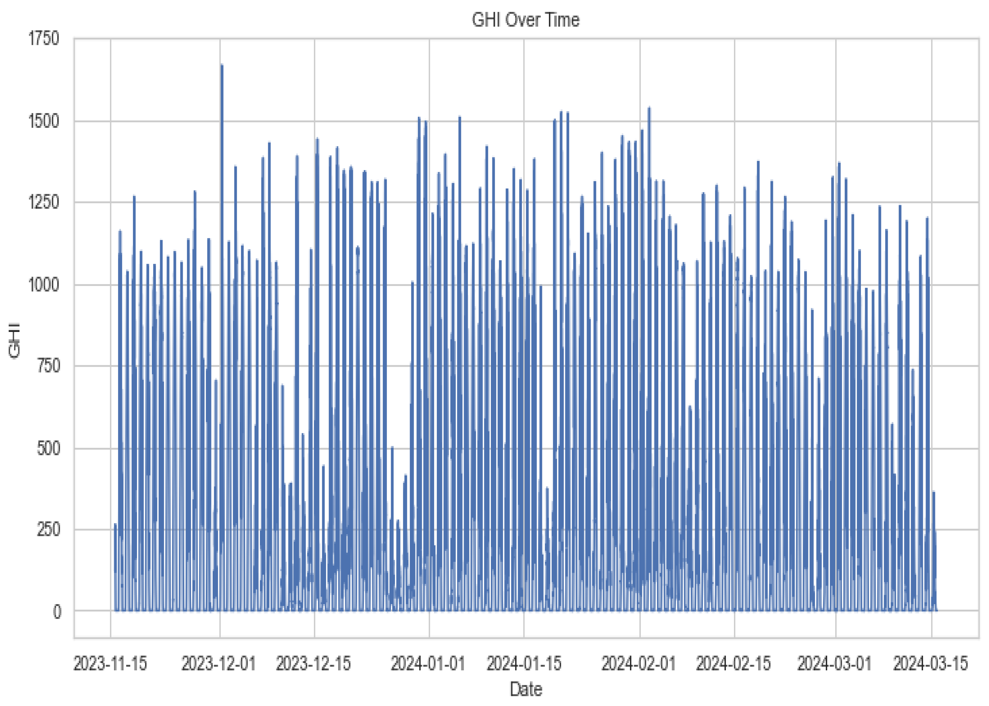
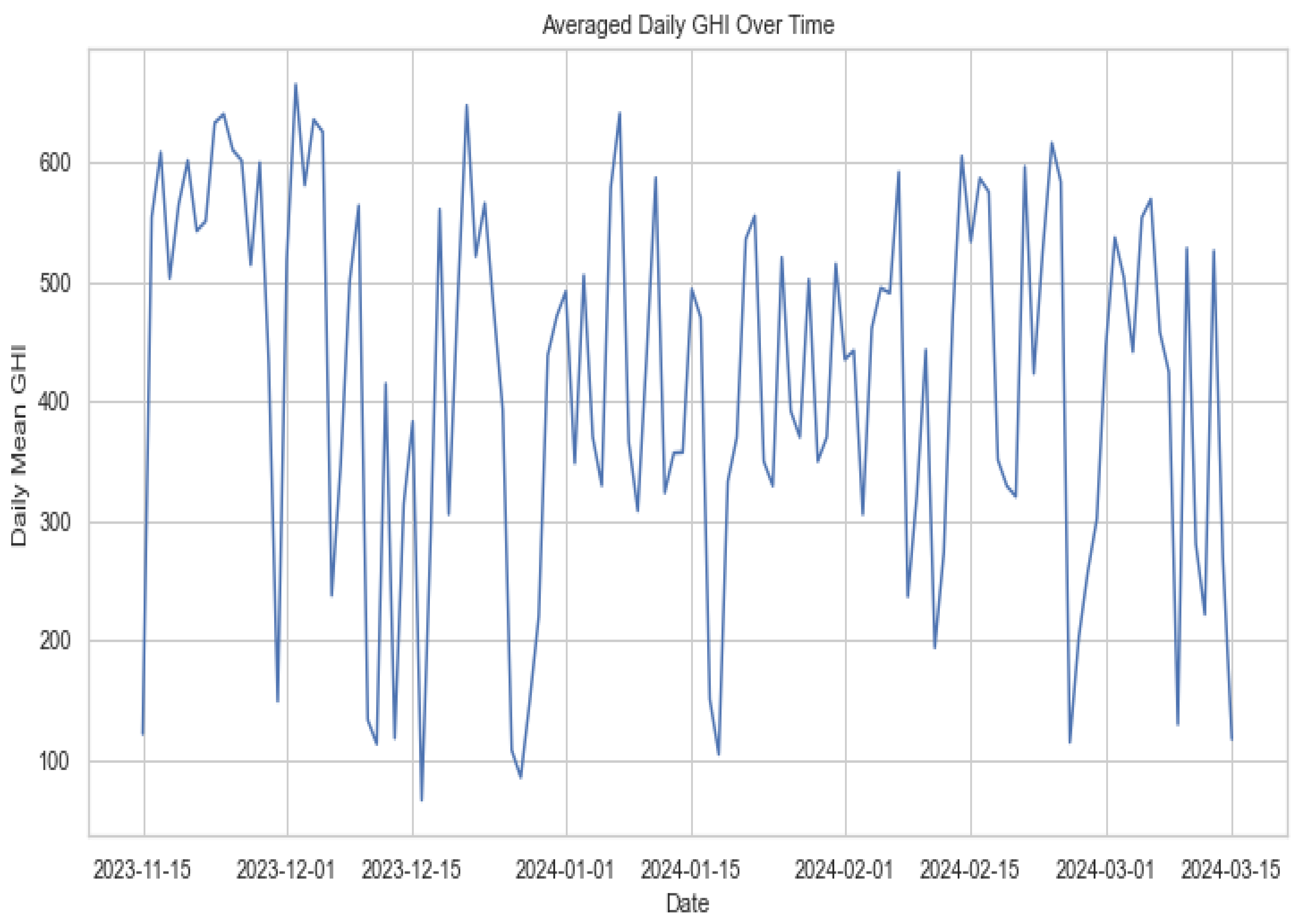
3.2. Exploratory Data Analysis

In our data preprocessing, we focused on cleaning the dataset to ensure its accuracy and reliability. One challenge we encountered was the presence of zero values in the GHI variable, which measures the total amount of shortwave radiation received from above by a horizontal surface. Since data were collected over 24 h, zero values were recorded during nighttime when there was no sunlight. To address this issue, we used listwise deletion to remove all the zero values based on GHI. This ensures that our study is robust. Imputation techniques were not considered, as simply replacing with a mean can introduce bias, as GHI depends on specific factors. Since GHI rises in the morning and peaks during the day, replacing it with mean or other values would reduce the quality of the study.

The summary statistics for the GHI data are presented in

Table 2. Summary statistics for GHI.

Min	Q1	Median	Mean	Q3	Max	Std	Skewness	Kurtosis
0.006	103.463	314.610	415.996	692.425	1666.725	359.767	0.653	−0.811

. These statistics provide a summary understanding of the variable before making predictions. The table includes the minimum, first quartile (Q1), mean, median, third quartile (Q3), maximum, standard deviation, skewness, and kurtosis. The GHI values in the dataset range from a minimum of 0.006 to a maximum of 1666.725, with an average value of 415.996 over the data period. This wide range of values indicates that the dataset captures various weather conditions, ranging from very low solar radiation during early mornings or overcast days to much higher levels during clear, sunny periods. The positive skewness of the data suggests that most of the GHI values are on the lower end, with fewer high values, which is typical for solar data as low irradiance occurs more often than peak values.

Additionally, the kurtosis value of −0.811 indicates that the distribution is platykurtic, meaning it has a flatter peak and fewer extreme outliers than a normal distribution. This suggests that while the GHI values vary, there are fewer extremely high or low values than expected, making the dataset more balanced and stable overall. Understanding these aspects of the data is crucial before proceeding with any predictive modelling.

3.3. Visualisations

Figure 2, Figure 3, Figure 4 and Figure 5 represent the GHI at different times, including the overall time, average daily aggregation, monthly aggregation, and by the hour. These plots allow us to observe the behaviour of GHI at different times. Figure 2 shows how GHI behaves minute by minute throughout the data, while Figure 3 displays the average daily GHI behaviour. Figure 5 summarises the GHI over different months covered by the data, revealing the highest GHI in the eleventh month of 2023. Lastly, Figure 4 illustrates the behaviour of GHI over hours, confirming that GHI is lowest during late hours and peaks during mid-hours of the data. These plots offer a comprehensive understanding of GHI trends across different time frames.

Figure 6 displays the density and Q-Q plots, confirming the earlier EDA findings. The density plot indicates a right-skewed distribution, with most GHI values between 0 and 200 and fewer high values above 1000. The Q-Q plot further illustrates that the GHI data deviate from normality, showing significant skewness and potential outliers, reinforcing that the data do not follow a normal distribution.

In Figure 7, a box plot illustrates the distribution of GHI across different time frames. The “GHI by Week of the Year” plot indicates that some weeks have high median GHI values, suggesting consistently sunny conditions. In contrast, other weeks display lower medians, indicating more overcast conditions. Numerous outliers, particularly in certain weeks, suggest occasional spikes in GHI, likely due to clear days occurring within otherwise variable weeks. The “GHI by Days of the Month” plot highlights the variation of GHI across individual days within a month. While the median GHI remains relatively stable, some days exhibit higher peaks or more outliers, indicating occasional increases in solar irradiance resulting from day-to-day weather fluctuations. Finally, the “GHI by Month of the Year” plot reveals seasonal trends, with some months demonstrating higher median GHI, reflecting sunnier seasons, while others show lower medians, indicative of cloudier periods. The outliers observed in certain months suggest occasional days of high irradiance, even during typically low-GHI months.

Figure 8 below displays the Autocorrelation Function (ACF) and the Partial Autocorrelation Function (PACF) plot for GHI. The ACF plot shows a slow, gradual decay in correlation, indicating that the time series is non-stationary and has long-term dependencies or trends. The strong correlations at multiple lags suggest that GHI values over time are highly persistent. On the other hand, the PACF plot shows a sharp cutoff after lag 1, suggesting that after accounting for the first lag, the correlations with subsequent lags are negligible.

In exploring the dataset, it is important to check how the dependent variable is correlated with other variables. After computing the correlation heatmap, Figure 9 shows that GHI is not correlated with any other variable. This insight prompts us to include all other variables in our analysis further.

3.4. Variable Selection

Figure 10 shows the selected feature’s importance. To achieve this, a Random Forest model was trained, and the feature importances were used to select the best set of features according to Recursive Feature Elimination with Cross-Validation (RFE-CV). The optimised metric was the negative mean squared error, and using five-fold cross-validation indicated that WVEC_mag, WS_Max, and WS do not significantly contribute to predicting GHI. Hence, these features will not be used in any models going forward.

3.5. Machine Learning Models

We trained various machine learning models after splitting the data into a 70–30 ratio. The data were normalised, and Bayesian optimisation was implemented to help train the models to use optimal hyperparameters. The results of the machine learning models’ performance on the test set are presented in Figure 11. These plots depict the machine learning model’s performance on the test set.

3.6. Selected Parameters

For the RNN model, the selected parameters from Bayesian optimisation are as follows: 32 units, a dropout rate of 0.2, a learning rate of 0.01, and 10 epochs.

For the RF model, the parameters are as follows: max depth of 50, max features of 0.6897487361224869, min samples leaf of 10, min samples split of 10, and n estimators of 200.

For the GB model, the selected parameters are as follows: learning rate of 0.01, max depth of four, min samples leaf of six, min samples split of 13, n estimators of 474, and a subsample of 0.8670322417190656. Finally, for the SVR model, the selected parameters are the following: best C of 100.0 and best epsilon of 0.01.

3.7. Model Comparison

Table 3. Machine learning model comparison.

	MAE	RMAE	RMSE	RRMSE
RNN	22.1037	0.4290	25.6224	0.4973
SVR	26.4253	0.0668	81.9700	0.2073
RF	28.9002	0.0730	79.6583	0.2014
GB	29.6836	0.0750	78.0158	0.1973

compares four machine learning models: RNN, SVR, RF, and GB. It evaluates their performance using four key metrics: MAE and RMSE, which are measured in W/m², and RMAE and RRMSE, which are unitless. These metrics help assess the predictive accuracy of each model, with lower values generally indicating better performance in terms of prediction error. We calculated these metrics on the test set after training the models.

Among the models, the RNN demonstrates superior performance, achieving the lowest MAE of 22.1037 and RMSE of 25.6224. These low error values indicate that the RNN is the most accurate model in terms of both absolute and squared prediction errors. The RNN also exhibits the lowest relative errors, with an RMAE of 0.4290. These relative error metrics further highlight that the RNN model effectively minimises errors in absolute terms and maintains consistency and reliability across different prediction scales.

The SVR, RF, and GB models have higher error rates. The SVR model has a relatively low RMAE of 0.0668 but a much higher RMSE of 81.9700, indicating significant variability in its predictions and a higher penalty for larger errors. The RF and GB models have slightly better RMSE values (79.6583 and 78.0158, respectively) than SVR but still significantly lag behind the RNN model. The RF model’s MAE is 28.9002, and the GB model’s MAE is 29.6836. Their RMAE and RRMSE values (around 0.0730 and 0.0750 for RMAE and 0.2014 and 0.1973 for RRMSE, respectively) indicate that while these models perform reasonably well, they do not match the predictive accuracy or consistency demonstrated by the RNN model.

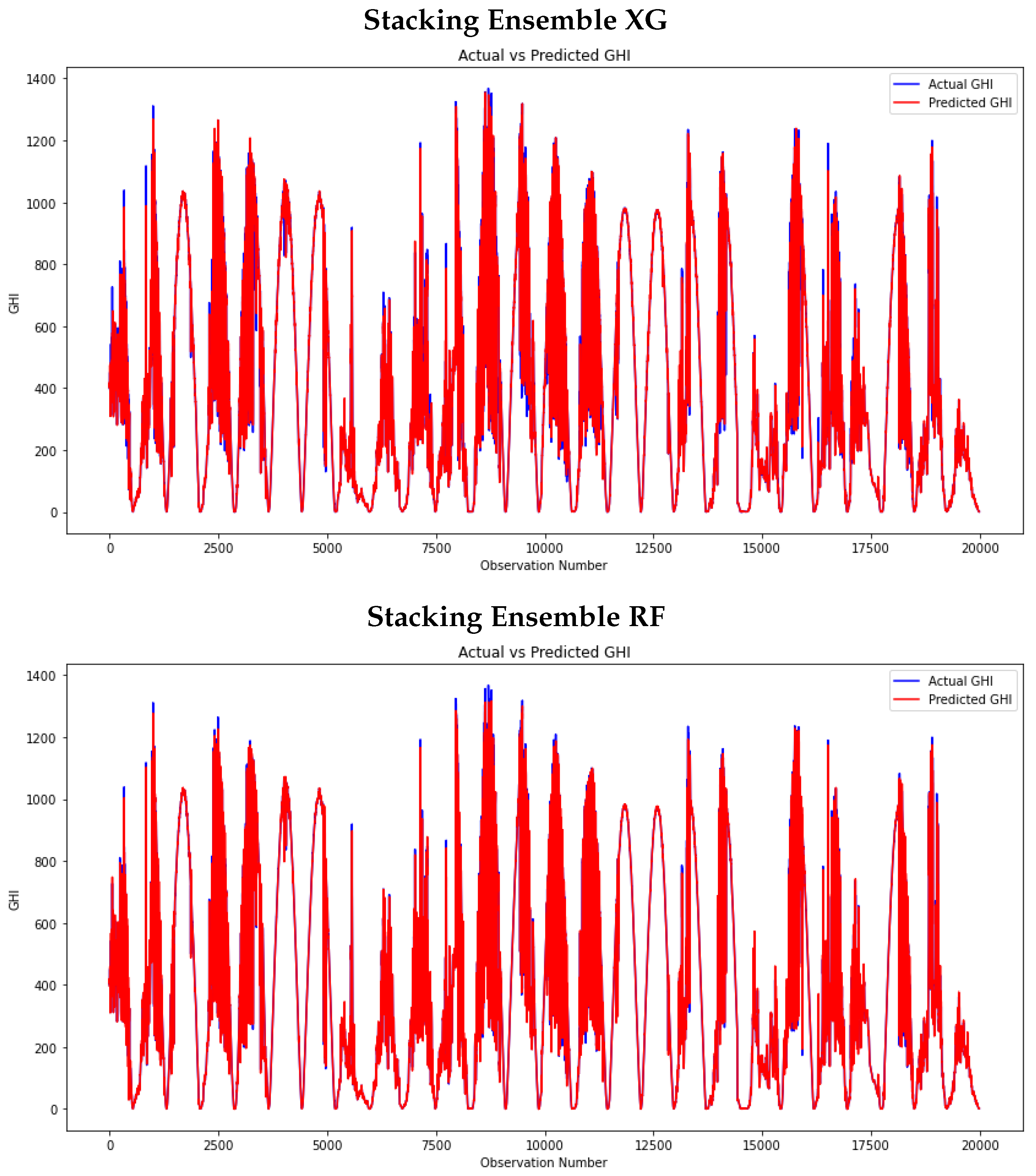
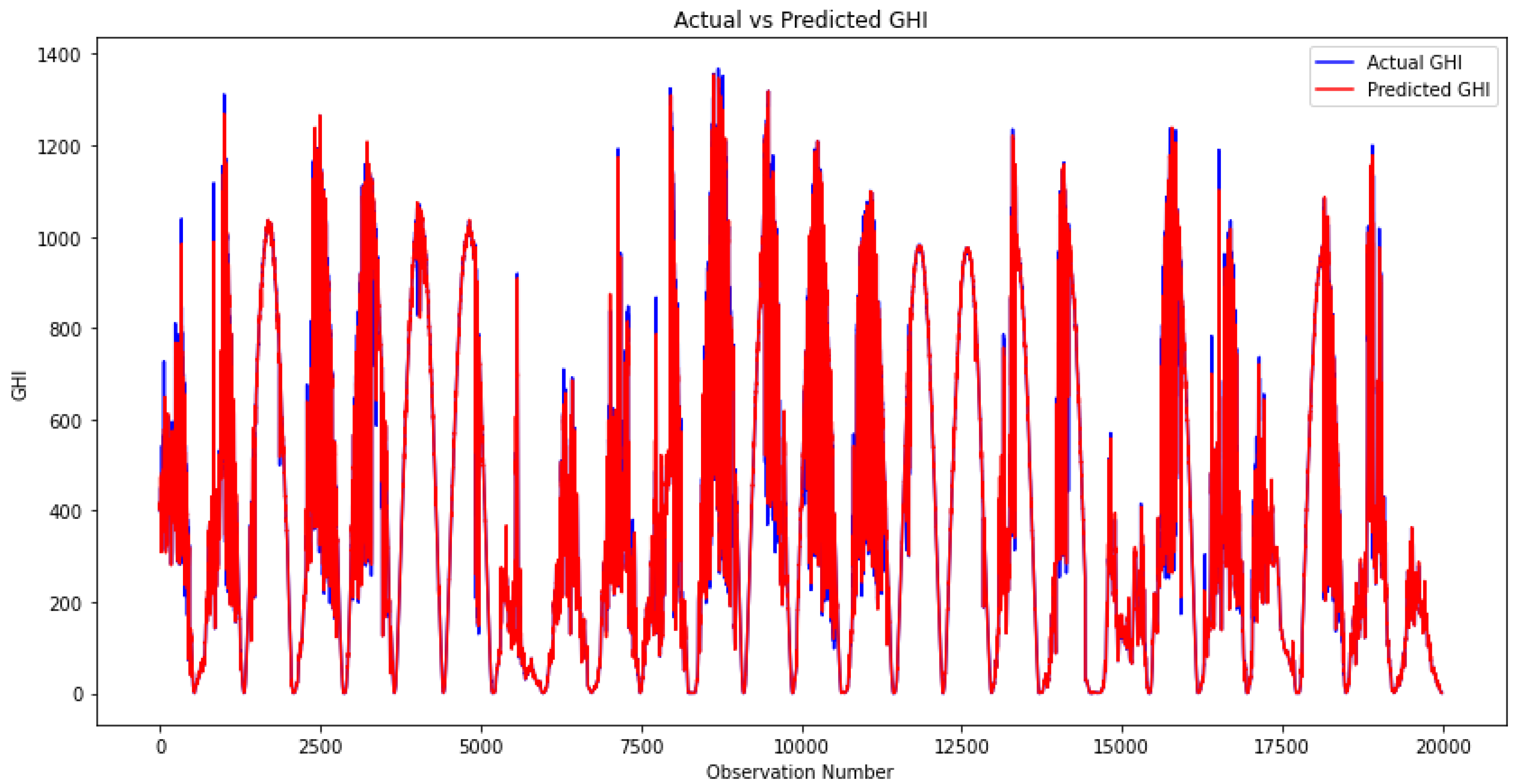
3.8. Stacking Ensemble Models

The study proceeded to train Stacking Ensemble models. This process began by using the same hyperparameters used in the individual machine learning models to provide a fair comparison of the models. In Section 3, there was a discussion of meta-models, which are essential for use in stacking learning models. Out of the four models mentioned, a mini experiment was conducted to select only two: RF and XGBOOST, as they are the top two meta-models. The Stacking Ensemble and the DNS model will further explore these models. Figure 12 and Figure 13 show the performance of the Stacking Ensemble and DNS models on the test set.

3.9. Model Comparison

In

Table 4. Stacking model comparison.

	MAE	RMAE	RMSE	RRMSE
SE XG	7.2808	0.0184	19.9125	0.0504
SE RF	11.7188	0.0296	30.6534	0.0775
DNS XG	5.0633	0.0128	16.0328	0.0406
DNS RF	2.9217	0.0074	7.5926	0.0192
DNS XG RF	4.5771	0.0116	11.8832	0.0301
DNS RF XG	1.5369	0.0038	2.9341	0.0074

, the error metrics for the Stacking Ensemble on the test set are displayed: MAE and RMSE, which are measured in W/m², and RMAE and RRMSE, which are unitless. The Stacking Ensemble with RF as the meta-model (SE RF) exhibits higher MAE and RMSE values than other models. This suggests that the SE RF model has larger prediction errors on average. The RMAE and RRMSE values also indicate a relatively high error proportion relative to the magnitude of the data. This might imply that the RF model is not as effective as other models in capturing the complexity or patterns in the data.

The Stacking Ensemble with XGBoost as the meta-model (SE XG) performed better than SE RF, showing significantly lower MAE, RMAE, RMSE, and RRMSE values. This suggests higher overall accuracy and lower error rates. The XGBoost meta-model may have utilised its Gradient Boosting mechanism to capture non-linear relationships and interactions among features better, resulting in a more accurate model than the RF meta-model.

The DNS model with RF as the meta-model (DNS RF) significantly improves over the SE RF model. The MAE and RMSE are much lower, indicating a substantial reduction in prediction errors. The RMAE and RRMSE values are also very low, suggesting high accuracy. This improvement may be attributed to the double nested structure, which enables the model to integrate predictions from different base learners better, resulting in more robust predictions.

The DNS XG model performs worse than the DNS RF model but better than the SE RF and SE XG models. Although XGBoost is generally a strong learner, the Double Nested Stacking framework with XGBoost does not outperform the RF meta-model in this setup. This could suggest that while XGBoost is powerful, it may not always yield the best results in ensemble frameworks involving multiple layers of modelling.

3.10. Meta-Model Order Impact

The order in which meta-models are arranged in DNS significantly impacts model performance. This is because each meta-model processes the predictions from base models differently. The output of one meta-model serves as the input for the next, thereby affecting the overall results. We conducted experiments to assess the effects of varying the sequence of meta-models in DNS, as displayed in Table 4.

The results of the experiments showed that the model using RF as the first meta-model, followed by XGBoost (DNS RF XG), performed better than the reverse order (DNS XG RF). Specifically, the MAE for DNS RF XG was 66.42% lower compared to DNS XG RF, and the RMSE was 75.31% lower. This indicates the significant impact of meta-model sequencing on the effectiveness of Double Nested Stacking models.

Figure 14 and Figure 15 show the performance of the DNS RF XG and DNS XG RF models on the test set.

4. Discussion

Forecasting GHI is crucial for measuring the potential solar energy production on a horizontal surface. This helps various sectors identify the best time to collect solar energy and plan for additional sourcing. The research project focuses on forecasting GHI using minute-averaged data from the SAURAN database for USAID Venda from 15 November 2023 to 15 March 2024.

In the previous section, we discussed modelling minute-averaged GHI forecasting using RNN, SVR, RF, GB, and two Stacking Ensemble methods. We also discussed the importance of variable selection and how we implemented RF, excluding three variables (wind speed, maximum wind speed, and wvec mag) from the GHI forecasting models.

After all the minute-averaged data preprocessing, including implementing hyperparameter tuning for each model using Bayesian optimisation, the results show that the best-performing machine learning model is the RNN because it has the lowest values for both MAE and RMSE. The second-best performing model is SVR, which has the second-lowest MAE after RNN. Although its RMSE is higher, it still outperforms both RF and GB models.

When evaluating the performance of the Stacking Ensemble models, it was important to use the same parameters selected during the individual models’ training. Four meta-models were used: Ridge regression, XGBOOST, RF, and Elastic Net. Out of these, the two best meta-models, RF and XGboost, were further explored to understand the impact of the meta-model in the Stacking Ensemble setting. The results showed that both Stacking Ensemble models with these meta-models outperformed all other machine learning models. The best stacking model was the one with XGboost as the meta-model, showing a 67.060% and 22.2848% increase in accuracy compared to the MAE and RMSE of the best-performing machine learning model, RNN.

Implementing the same meta-models in another stacking technique, DNS, revealed that accuracy can be further improved. The results showed that DNS XG and DNS RF outperform the single stacking model. The best-performing results show a decrease in MAE and RMSE by 59.87% and 61.87%, respectively, when compared to the best-performing SE XG. Further experimenting with the order and mixing of the meta-models can again improve the forecasting accuracy of the DNS model.

When the RF was the first-level meta-model followed by XGBOOST, the DNS model outperformed every model in the study, including the reverse order of the meta-models. The results show a 93.05% decrease in MAE and an 88.54% decrease in RMSE compared to the best-performing machine learning model and a 78.89% decrease in MAE and an 85.27% decrease in RMSE compared to the best single stacking model. Additionally, the DNS model outperformed DNS RF, where RF was used at both levels, showing a decrease in MAE and RMSE by 47.39% and 61.35%, respectively.

The results from the Stacking Ensemble models showed consistency and indicated that these models outperformed traditional machine learning approaches [9]. Furthermore, our findings support those of [10], which stated that the DNS model surpassed the stacking ensemble.

A significant advancement in our study was the experimentation with various meta-models and their configurations within the ensemble. This exploration demonstrated that modifying the meta-models and their arrangements improves model accuracy, underscoring the methodological advancements made in this research.

5. Conclusions

Machine learning models can provide fairly accurate forecasts for GHI. However, implementing advanced techniques such as Stacking Ensembles with multiple levels and experimenting with different meta-models can significantly improve performance. The results demonstrate the potential of stacking, which has been validated in other sectors. This study highlights its promising application in the renewable energy sector.

References

1. Demirbas, A. Recent advances in biomass conversion technologies. Energy Educ. Sci. Technol. 2000, 6, 19–41. [Google Scholar]
2. Armaroli, N.; Balzani, V. The legacy of fossil fuels. Chem. Asian J. 2011, 6, 768–784. [Google Scholar] [CrossRef] [PubMed]
3. Gbémou, S.; Eynard, J.; Thil, S.; Guillot, E.; Grieu, S. A comparative study of machine learning-based methods for global horizontal irradiance forecasting. Energies 2021, 14, 3192. [Google Scholar] [CrossRef]
4. Rajaprasad, S.V.S.; Mukkamala, R. A hybrid deep learning framework for modeling the short term global horizontal irradiance prediction of a solar power plant in India. Polityka-Energetyczna-Energy Policy J. 2023, 26, 101–116. [Google Scholar] [CrossRef]
5. Yamani, A.Z.; Alyami, S.N. Investigating Hourly Global Horizontal Irradiance Forecasting Using Long Short-Term Memory. In Proceedings of the 2021 IEEE Asia-Pacific Conference on Computer Science and Data Engineering (CSDE), Brisbane, Australia, 8–10 December 2021; pp. 1–6. [Google Scholar] [CrossRef]
6. Benali, L.; Notton, G. A Fouilloy, Cyril Voyant, and Rabah Dizene. Solar radiation forecasting using artificial neural network and random forest methods: Application to normal beam, horizontal diffuse and global components. Renew. Energy 2019, 132, 871–884. [Google Scholar] [CrossRef]
7. Krishnan, N.; Kumar, K.R.; Anirudh R., S. Solar Radiation Forecasting using Gradient Boosting based Ensemble Learning Model for Various Climatic Zones. Sustain. Energy Grids Netw. 2024, 38, 101312. [Google Scholar] [CrossRef]
8. Nziyumva, E.; Nsengimna, M.; Niyogisubizo, J.; Murwanashyaka, E.; Nisingizwe, E.; Kwitonda, A. A Novel Two Layer Stacking Ensemble for Improving Solar Irradiance Forecasting. Int. J. Eng. Res. Technol. (IJERT) 2023, 10, 364–373. Available online: https://www.ijert.org/a-novel-two-layer-stacking-ensemble-for-improving-solar-irradiance-forecasting (accessed on 25 August 2024).
9. Guo, X.; Gao, Y.; Zheng, D.; Ning, Y.; Zhao, Q. Study on short-term photovoltaic power prediction model based on the Stacking Ensemble learning. Energy Rep. 2020, 6, 1424–1431. [Google Scholar] [CrossRef]
10. Zhou, B.; Chen, X.; Li, G.; Gu, P.; Huang, J.; Yang, B. Xgboost—sfs and Double Nested Stacking Ensemble model for photovoltaic power forecasting under variable weather conditions. Sustainability 2023, 15, 13146. [Google Scholar] [CrossRef]
11. Mandic, D.P.; Chambers, J. Recurrent Neural Networks for Prediction: Learning Algorithms, Architectures and Stability; John Wiley & Sons, Inc.: Hoboken, NJ, USA, 2001. [Google Scholar] [CrossRef]
12. Garcia-Pedrero, A.; Gomez-Gil, P. Time series forecasting using recurrent neural networks and wavelet reconstructed signals. In Proceedings of the 2010 20th International Conference on Electronics Communications and Computers (CONIELECOMP), Cholula, Puebla, Mexico, 22–24 February 2010; pp. 169–173. [Google Scholar] [CrossRef]
13. Vapnik, V.N. Statistical Learning Theory; Wiley: New York, NY, USA, 1998; ISBN 978-0-471-03003-4. [Google Scholar]
14. Drucker, H.; Burges, C.J.; Kaufman, L.; Smola, A.; Vapnik, V. Support vector regression machines. Adv. Neural Inf. Process. Syst. 1996, 9, 156–161. Available online: https://proceedings.neurips.cc/paper_files/paper/1996/file/d38901788c533e8286cb6400b40b386d-Paper.pdf (accessed on 27 May 2024).
15. Aghelpour, P.; Mohammadi, B.; Biazar, S.M. Long-term monthly average temperature forecasting in some climate types of Iran, using the models SARIMA, SVR, and SVR-FA. Theor. Appl. Climatol. 2019, 138, 1471–1480. [Google Scholar] [CrossRef]
16. Breiman, L.; Ihaka, R. Nonlinear Discriminant Analysis via Scaling and ACE; Department of Statistics, University of California Davis One Shields Avenue: Davis, CA, USA, 1984; Available online: https://www.stat.berkeley.edu/~breiman/nldiscanace.pdf (accessed on 14 June 2024).
17. Breiman, L. Random forests. Mach. Learn. 2001, 45, 5–32. [Google Scholar] [CrossRef]
18. Lahouar, A.; Slama, J.B.H. Random forests model for one day ahead load forecasting. In Proceedings of the IREC2015 the Sixth International Renewable Energy Congress, Sousse, Tunisia, 24–26 March 2015; pp. 1–6. [Google Scholar] [CrossRef]
19. Friedman, J.H. Greedy function approximation: A gradient boosting machine. Ann. Stat. 2001, 29, 1189–1232. Available online: https://www.jstor.org/stable/2699986 (accessed on 3 August 2024). [CrossRef]
20. Nemalili, R.C.; Jhamba, L.; Kirui, J.K.; Sigauke, C. Nowcasting Hourly-Averaged Tilt Angles of Acceptance for Solar Collector Applications Using Machine Learning Models. Energies 2023, 16, 927. [Google Scholar] [CrossRef]
21. Alcántara, A.; Galván, I.M.; Aler, R. Deep neural networks for the quantile estimation of regional renewable energy production. Appl. Intell. 2023, 53, 8318–8353. [Google Scholar] [CrossRef]
22. Wolpert, D.H. Stacked generalization. Neural Netw. 1992, 5, 241–259. [Google Scholar] [CrossRef]
23. van der Laan, M.J.; Polley, E.C.; Hubbard, A.E. Super Learner. Stat. Appl. Genet. Mol. Biol. 2007, 6. [Google Scholar] [CrossRef]
24. Khandelwal, Y. Ensemble stacking for machine learning and deep learning. Anal. Vidhya 2021, 9. Available online: https://www.analyticsvidhya.com/blog/2021/08/ensemble-stacking-for-machine-learning-and-deep-learning/ (accessed on 24 May 2024).
25. Divina, F.; Gilson, A.; Goméz-Vela, F.; Torres, M.G.; Torres, J.F. Stacking Ensemble learning for short-term electricity consumption forecasting. Energies 2018, 11, 949. [Google Scholar] [CrossRef]
26. Joy, T.T.; Rana, S.; Gupta, S.; Venkatesh, S. Hyperparameter tuning for big data using Bayesian optimisation. In Proceedings of the 2016 23rd International Conference on Pattern Recognition (ICPR), Cancun, Mexico, 4–8 December 2016; pp. 2574–2579. [Google Scholar] [CrossRef]
27. Gardner, J.R.; Kusner, M.J.; Xu, Z.E.; Weinberger, K.Q.; Cunningham, J.P. Bayesian optimization with inequality constraints. ICML 2014, 2014, 937–945. Available online: https://proceedings.mlr.press/v32/gardner14.pdf (accessed on 13 July 2024).
28. Fox, E.W.; Hill, R.A.; Leibowitz, S.G.; Olsen, A.R.; Thornbrugh, D.J.; Weber, M.H. Assessing the accuracy and stability of variable selection methods for random forest modeling in ecology. Environ. Monit. Assess. 2017, 189, 316. [Google Scholar] [CrossRef] [PubMed]
29. Genuer, R.; Poggi, J.-M.; Tuleau-Malot, C. Variable selection using random forests. Pattern Recognit. Lett. 2010, 31, 2225–2236. [Google Scholar] [CrossRef]
Figure 1. Flowchart of Stacking Ensemble modelling framework.
Computation 13 00072 g001
Figure 2. GHI for sampling period 2023 to 2024.
Computation 13 00072 g002
Figure 3. Averaged daily GHI.
Computation 13 00072 g003
Figure 4. GHI over hours.
Computation 13 00072 g004
Figure 5. GHI over months.
Computation 13 00072 g005
Figure 6. Density and QQ plot.
Computation 13 00072 g006
Figure 7. Distribution of GHI across the week, day, hour and month in the dataset.
Computation 13 00072 g007
Figure 8. ACF and PACF plots.
Computation 13 00072 g008
Figure 9. Correlation of the dataset.
Computation 13 00072 g009
Figure 10. Feature selections.
Computation 13 00072 g010
Figure 11. Machine learning model performance on test set.
Computation 13 00072 g011aComputation 13 00072 g011b
Figure 12. Stacking Ensemble performance on test set.
Computation 13 00072 g012
Figure 13. DNS model performance on test set.
Computation 13 00072 g013
Figure 14. DNS XG-RF.
Computation 13 00072 g014
Figure 15. DNS RF-XG.
Computation 13 00072 g015