Novel Techniques with Memory Extension of Three-Step Derivative-Free Iterative Scheme for Nonlinear Systems

Abstract

This article presents the development of three-step derivative-free techniques with memory, which achieve higher convergence orders for solving systems of nonlinear equations. The suggested approaches enhance an existing seventh-order method (without memory) by incorporating various adjustable, self-correcting parameters in the first iterative step. This modification leads to a significant increase in the convergence order, with new methods reaching values of approximately $7.2749$, $7.5311$, $7.6056$, $8.1231$, $8.2749$, and $9.2169$. Additionally, the computational efficiency of these new approaches is evaluated against other comparable methods. Numerical tests show that the suggested approaches are consistently more efficient.

1. Introduction

In many real-world engineering and scientific problems, it is common to encounter equations of the form $G\left(r\right)=0$, where $G:D\subset {\mathbb{R}}^n\to {\mathbb{R}}^n$ and D represents a neighborhood around a solution of $G\left(r\right)=0$. These equations are often difficult to solve exactly, so the goal is to find approximate solutions. In these situations, iterative approaches are helpful because they produce a series of approximations $\left\{r_k\right\}$ that, under specific circumstances, converge to the system’s actual solution.

Among various iterative methods, Newton’s procedure is particularly notable. It can be expressed as follows:

$$r^{(k+1)}=r^{\left(k\right)}-{\left[G^{\prime }\left(r^{\left(k\right)}\right)\right]}^{-1}G\left(r^{\left(k\right)}\right),$$

(1)

where $G^{\prime }\left(r^{\left(k\right)}\right)$ represents the Jacobian matrix associated with G. Newton’s approach is well known for its remarkable quadratic convergence rate, straightforwardness, and effectiveness. An alternative method, Steffensen’s method, arises when the derivative in the Newtonian scheme is substituted with the divided difference $[r+G(r),r;G]$. As discussed in reference [1], Steffensen’s method is a derivative-free iterative approach that demonstrates quadratic convergence. In contrast, methods like Newton’s require the computation of the derivative $G^{\prime }$ in the iterative formula. This requirement poses challenges when dealing with non-differentiable functions, when the computation of derivatives is costly, or when the Jacobian matrix is singular.

Various methods similar to Newton’s have been devised, which employ distinct techniques such as weight functions, direct composition, and estimations of Jacobian matrices through divided difference operators. Consequently, several iterative approaches for approximating solutions to $G\left(r\right)=0$ have been scrutinized, each exhibiting distinct orders of convergence. These proposals aim to enhance convergence speed or refine computational efficiency.

Recent studies [2,3,4] have introduced novel parametric classes of iterative techniques, which provide a rapid approach for addressing such problems. Moreover, previous works [5,6] have proposed several iterative methods that eliminate the necessity for the Jacobian matrix while showing advantageous rates of convergence. These methods replace the Jacobian matrix $G^{\prime }(-)$ with the divided difference operator $[-,-;G]$. In addition, the comprehensive work by Argyros [7] provides a detailed theoretical foundation for iterative methods, discussing their convergence properties, computational aspects, and broad range of applications. This resource serves as a cornerstone for advancing iterative techniques in solving nonlinear equations and systems.

Motivation: Computing the Jacobian matrix for derivative-based iterative methods when solving nonlinear systems, especially in higher dimensions, is a challenging task. This is why derivative-free iterative methods are often preferred as they avoid the need for computing derivatives. Additionally, the incorporation of memory techniques in iterative methods can significantly improve the convergence rate without requiring extra function evaluations. This is why we are particularly interested in methods with memory as they offer enhanced performance compared to those without memory. While there are a few studies on derivative-free iterative techniques with memory, most of the existing literature focuses on methods without memory. This gap in the literature motivates our research to explore and develop derivative-free iterative techniques with memory, which can offer superior convergence properties.

Novelty of the paper: Author: Yes, bold is removed. The novelty of this research lies in the development of new derivative-free iterative schemes with memory, which achieve more than ninth-order convergence. It improves existing seventh-order iterative methods while minimizing computational costs. These methods are specifically designed to reduce the quantity of function evaluations and eliminate the need for the costly inversion of Jacobian matrices. By striking a balance between computational efficiency and high convergence rates, the proposed techniques offer significant advancements over current methods.

The structure of our presentation is as follows: The new techniques are presented, and a convergence study is conducted in Section 2. The computational efficiency of these approaches is evaluated in Section 3, which also provides a broad comparison with a number of well-known algorithms. Numerous numerical examples are provided in Section 4 in order to verify the theoretical conclusions and compare the convergence characteristics of the suggested approaches with those of other comparable, well-established approaches. Lastly, Section 5 concludes with final remarks.

2. With Memory Method and Its Convergence Analysis

In the subsequent section, we concentrate on optimizing the parameter $\beta$ in the iterative technique suggested by Sharma and Arora [8] to improve its convergence rate. We start by examining the seventh-order method without memory, as described in the cited work [8].

$$\begin{array}{cc}\hfill p^{\left(k\right)}& =r^{\left(k\right)}-{[t^{\left(k\right)},r^{\left(k\right)};G]}^{-1}G\left(r^{\left(k\right)}\right),\hfill \\ \hfill q^{\left(k\right)}& =p^{\left(k\right)}-\left(3I-{[t^{\left(k\right)},r^{\left(k\right)};G]}^{-1}\left([p^{\left(k\right)},r^{\left(k\right)};G]+[p^{\left(k\right)},t^{\left(k\right)};G]\right)\right){[t^{\left(k\right)},r^{\left(k\right)};G]}^{-1}G\left(p^{\left(k\right)}\right),\hfill \\ \hfill r^{(k+1)}& =q^{\left(k\right)}-{[q^{\left(k\right)},p^{\left(k\right)};G]}^{-1}\left([t^{\left(k\right)},r^{\left(k\right)};G]+[p^{\left(k\right)},r^{\left(k\right)};G]-[q^{\left(k\right)},r^{\left(k\right)};G]\right)\hfill \\ & \times {[t^{\left(k\right)},r^{\left(k\right)};G]}^{-1}G\left(q^{\left(k\right)}\right).\hfill \end{array}$$

(2)

Here, $t^{\left(k\right)}=r^{\left(k\right)}+\beta G\left(r^{\left(k\right)}\right)$ and it is denoted by $M_7$. The error expressions for the sub-steps of the above-mentioned method are as follows:

$$\begin{array}{cc}\hfill e^{(p,k)}& =(I+\beta G^{\prime }\left(\alpha \right))A_2{\left(e^{\left(k\right)}\right)}^2,\hfill \end{array}$$

(3)

$$\begin{array}{cc}\hfill e^{(q,k)}& =(I+\beta G^{\prime }\left(\alpha \right))A_2{\left(e^{\left(k\right)}\right)}^4,\hfill \end{array}$$

(4)

$$\begin{array}{cc}\hfill e^{(k+1)}& ={(I+\beta G^{\prime }\left(\alpha \right))}^2{A}_2^{2}Q{\left(e^{\left(k\right)}\right)}^7,\hfill \end{array}$$

(5)

where $Q=((2I+\beta G^{\prime }\left(\alpha \right))A_2^2-A_3)((5I+\beta G^{\prime }\left(\alpha \right)(5I+\beta G^{\prime }\left(\alpha \right)))A_2^2-(I+\beta G^{\prime }\left(\alpha \right))A_3)$, $e^{(k+1)}=r^{(k+1)}-\alpha$, $A_i={\displaystyle \frac{1}{i!}}{\left[G^{\prime }\left(\alpha \right)\right]}^{-1}{G}^{\left(i\right)}\left(\alpha \right)$. Let $\alpha$ be a root of the nonlinear system $G\left(r\right)=0$. From the error expression (5), it is apparent that the method achieves a convergence order of 7 when $\beta \ne -{\left[G^{\prime }\left(\alpha \right)\right]}^{-1}$. However, if we choose $\beta =-{\left[G^{\prime }\left(\alpha \right)\right]}^{-1}$, the convergence order can be improved to exceed nine. Since the precise value of $G^{\prime }\left(\alpha \right)$ is not directly accessible, we rely on an approximation of $G^{\prime }\left(\alpha \right)$ derived from the available data, which helps to further accelerate the convergence rate.

The fundamental idea behind developing memory-based methods is to iteratively compute the parameter matrix $\beta =B_i^{\left(k\right)}$ (for $k=1,2,\dots ,6,i=1,2,\dots ,6$) by using a sufficiently accurate approximation of ${\left[G^{\prime }\left(\alpha \right)\right]}^{-1}$, which is derived from the available information. We propose the following forms for this variable matrix parameter $B_i^{\left(k\right)}$:

• Scheme 1.

$$B_1^{\left(k\right)}=-{[t^{(k-1)},r^{(k-1)};G]}^{-1}.$$

(6)

• Scheme 2.

  $$B_2^{\left(k\right)}=-{[2r^{\left(k\right)}-r^{(k-1)},r^{(k-1)};G]}^{-1}.$$

  (7)

  this divided difference operator is also known as Kurchatov’s divided difference.

• Scheme 3.

$$B_3^{\left(k\right)}=-{[r^{\left(k\right)},p^{(k-1)};G]}^{-1}.$$

(8)

• Scheme 4.

$$B_4^{\left(k\right)}=-{[r^{\left(k\right)},q^{(k-1)};G]}^{-1}.$$

(9)

• Scheme 5.

$$B_5^{\left(k\right)}=-{[2r^{\left(k\right)}-p^{(k-1)},p^{(k-1)};G]}^{-1}.$$

(10)

• Scheme 6.

  $$B_6^{\left(k\right)}=-{[2r^{\left(k\right)}-q^{(k-1)},q^{(k-1)};G]}^{-1}.$$

  (11)

  By substituting the parameter $\beta$ in method (2) with schemes 1 through 6, we obtain six new three-step iterative methods with memory, which are described in detail as follows:

$$\left\{\begin{array}{cc}\hfill t^{\left(k\right)}& =r^{\left(k\right)}+B_1^{\left(k\right)}G\left(r^{\left(k\right)}\right),\hfill \\ \hfill p^{\left(k\right)}& =r^{\left(k\right)}-{[t^{\left(k\right)},r^{\left(k\right)};G]}^{-1}G\left(r^{\left(k\right)}\right),\hfill \\ \hfill q^{\left(k\right)}& =p^{\left(k\right)}-\left(3I-{[t^{\left(k\right)},r^{\left(k\right)};G]}^{-1}\left([p^{\left(k\right)},r^{\left(k\right)};G]+[p^{\left(k\right)},t^{\left(k\right)};G]\right)\right){[t^{\left(k\right)},r^{\left(k\right)};G]}^{-1}G\left(p^{\left(k\right)}\right),\hfill \\ \hfill r^{(k+1)}& =q^{\left(k\right)}-{[q^{\left(k\right)},p^{\left(k\right)};G]}^{-1}\left([t^{\left(k\right)},r^{\left(k\right)};G]+[p^{\left(k\right)},r^{\left(k\right)};G]-[q^{\left(k\right)},r^{\left(k\right)};G]\right)\hfill \\ & \times {[t^{\left(k\right)},r^{\left(k\right)};G]}^{-1}G\left(q^{\left(k\right)}\right).\hfill \end{array}\right.$$

(12)

$$\left\{\begin{array}{cc}\hfill t^{\left(k\right)}& =r^{\left(k\right)}+B_2^{\left(k\right)}G\left(r^{\left(k\right)}\right),\hfill \\ \hfill p^{\left(k\right)}& =r^{\left(k\right)}-{[t^{\left(k\right)},r^{\left(k\right)};G]}^{-1}G\left(r^{\left(k\right)}\right),\hfill \\ \hfill q^{\left(k\right)}& =p^{\left(k\right)}-\left(3I-{[t^{\left(k\right)},r^{\left(k\right)};G]}^{-1}\left([p^{\left(k\right)},r^{\left(k\right)};G]+[p^{\left(k\right)},t^{\left(k\right)};G]\right)\right){[t^{\left(k\right)},r^{\left(k\right)};G]}^{-1}G\left(p^{\left(k\right)}\right),\hfill \\ \hfill r^{(k+1)}& =q^{\left(k\right)}-{[q^{\left(k\right)},p^{\left(k\right)};G]}^{-1}\left([t^{\left(k\right)},r^{\left(k\right)};G]+[p^{\left(k\right)},r^{\left(k\right)};G]-[q^{\left(k\right)},r^{\left(k\right)};G]\right)\hfill \\ & \times {[t^{\left(k\right)},r^{\left(k\right)};G]}^{-1}G\left(q^{\left(k\right)}\right).\hfill \end{array}\right.$$

(13)

$$\left\{\begin{array}{cc}\hfill t^{\left(k\right)}& =r^{\left(k\right)}+B_3^{\left(k\right)}G\left(r^{\left(k\right)}\right),\hfill \\ \hfill p^{\left(k\right)}& =r^{\left(k\right)}-{[t^{\left(k\right)},r^{\left(k\right)};G]}^{-1}G\left(r^{\left(k\right)}\right),\hfill \\ \hfill q^{\left(k\right)}& =p^{\left(k\right)}-\left(3I-{[t^{\left(k\right)},r^{\left(k\right)};G]}^{-1}\left([p^{\left(k\right)},r^{\left(k\right)};G]+[p^{\left(k\right)},t^{\left(k\right)};G]\right)\right){[t^{\left(k\right)},r^{\left(k\right)};G]}^{-1}G\left(p^{\left(k\right)}\right),\hfill \\ \hfill r^{(k+1)}& =q^{\left(k\right)}-{[q^{\left(k\right)},p^{\left(k\right)};G]}^{-1}\left([t^{\left(k\right)},r^{\left(k\right)};G]+[p^{\left(k\right)},r^{\left(k\right)};G]-[q^{\left(k\right)},r^{\left(k\right)};G]\right)\hfill \\ & \times {[t^{\left(k\right)},r^{\left(k\right)};G]}^{-1}G\left(q^{\left(k\right)}\right).\hfill \end{array}\right.$$

(14)

$$\left\{\begin{array}{cc}\hfill t^{\left(k\right)}& =r^{\left(k\right)}+B_4^{\left(k\right)}G\left(r^{\left(k\right)}\right),\hfill \\ \hfill p^{\left(k\right)}& =r^{\left(k\right)}-{[t^{\left(k\right)},r^{\left(k\right)};G]}^{-1}G\left(r^{\left(k\right)}\right),\hfill \\ \hfill q^{\left(k\right)}& =p^{\left(k\right)}-\left(3I-{[t^{\left(k\right)},r^{\left(k\right)};G]}^{-1}\left([p^{\left(k\right)},r^{\left(k\right)};G]+[p^{\left(k\right)},t^{\left(k\right)};G]\right)\right){[t^{\left(k\right)},r^{\left(k\right)};G]}^{-1}G\left(p^{\left(k\right)}\right),\hfill \\ \hfill r^{(k+1)}& =q^{\left(k\right)}-{[q^{\left(k\right)},p^{\left(k\right)};G]}^{-1}\left([t^{\left(k\right)},r^{\left(k\right)};G]+[p^{\left(k\right)},r^{\left(k\right)};G]-[q^{\left(k\right)},r^{\left(k\right)};G]\right)\hfill \\ & \times {[t^{\left(k\right)},r^{\left(k\right)};G]}^{-1}G\left(q^{\left(k\right)}\right).\hfill \end{array}\right.$$

(15)

$$\left\{\begin{array}{cc}\hfill t^{\left(k\right)}& =r^{\left(k\right)}+B_5^{\left(k\right)}G\left(r^{\left(k\right)}\right),\hfill \\ \hfill p^{\left(k\right)}& =r^{\left(k\right)}-{[t^{\left(k\right)},r^{\left(k\right)};G]}^{-1}G\left(r^{\left(k\right)}\right),\hfill \\ \hfill q^{\left(k\right)}& =p^{\left(k\right)}-\left(3I-{[t^{\left(k\right)},r^{\left(k\right)};G]}^{-1}\left([p^{\left(k\right)},r^{\left(k\right)};G]+[p^{\left(k\right)},t^{\left(k\right)};G]\right)\right){[t^{\left(k\right)},r^{\left(k\right)};G]}^{-1}G\left(p^{\left(k\right)}\right),\hfill \\ \hfill r^{(k+1)}& =q^{\left(k\right)}-{[q^{\left(k\right)},p^{\left(k\right)};G]}^{-1}\left([t^{\left(k\right)},r^{\left(k\right)};G]+[p^{\left(k\right)},r^{\left(k\right)};G]-[q^{\left(k\right)},r^{\left(k\right)};G]\right)\hfill \\ & \times {[t^{\left(k\right)},r^{\left(k\right)};G]}^{-1}G\left(q^{\left(k\right)}\right).\hfill \end{array}\right.$$

(16)

$$\left\{\begin{array}{cc}\hfill t^{\left(k\right)}& =r^{\left(k\right)}+B_6^{\left(k\right)}G\left(r^{\left(k\right)}\right),\hfill \\ \hfill p^{\left(k\right)}& =r^{\left(k\right)}-{[t^{\left(k\right)},r^{\left(k\right)};G]}^{-1}G\left(r^{\left(k\right)}\right),\hfill \\ \hfill q^{\left(k\right)}& =p^{\left(k\right)}-\left(3I-{[t^{\left(k\right)},r^{\left(k\right)};G]}^{-1}\left([p^{\left(k\right)},r^{\left(k\right)};G]+[p^{\left(k\right)},t^{\left(k\right)};G]\right)\right){[t^{\left(k\right)},r^{\left(k\right)};G]}^{-1}G\left(p^{\left(k\right)}\right),\hfill \\ \hfill r^{(k+1)}& =q^{\left(k\right)}-{[q^{\left(k\right)},p^{\left(k\right)};G]}^{-1}\left([t^{\left(k\right)},r^{\left(k\right)};G]+[p^{\left(k\right)},r^{\left(k\right)};G]-[q^{\left(k\right)},r^{\left(k\right)};G]\right)\hfill \\ & \times {[t^{\left(k\right)},r^{\left(k\right)};G]}^{-1}G\left(q^{\left(k\right)}\right).\hfill \end{array}\right.$$

(17)

To evaluate the convergence properties of schemes (12)–(17), we need the following results related to Taylor expansions of vector functions (one can see the Refs. [9,10,11,12,13]).

Lemma 1.

Let $D\subset {\mathbb{R}}^m$ be a convex set, and let $G:D\subset {\mathbb{R}}^m\to {\mathbb{R}}^m$ be a function that is p-times Fréchet differentiable. Then, for any $r,h\in {\mathbb{R}}^m$, the function $G(r+h)$ can be expressed as follows:

$$G(r+h)=G\left(r\right)+G^{\prime }\left(r\right)h+{\displaystyle \frac{1}{2!}}{G}^{″}\left(r\right)h^2+{\displaystyle \frac{1}{3!}}{G}^{‴}\left(r\right)h^3+\dots +{\displaystyle \frac{1}{(p-1)!}}{G}^{(p-1)}\left(r\right)h^{p-1}+R_p,$$

where the remainder term $R_p$ satisfies the following inequality:

$$\parallel R_p\parallel \le {\displaystyle \frac{1}{p!}}\underset{0\le t\le 1}{sup}\parallel G^{\left(p\right)}{(r+th)\parallel \parallel h\parallel }^p,$$

and $h^p$ denotes the vector $(h,h,\dots ,h)$, with h repeated p times.

In our approach, we have used the divided difference operator for the multi-variable function G (see [9,14,15]). This operator, represented as $[.,.;G]$, is a mapping $D\times D\subset {\mathbb{R}}^m\times {\mathbb{R}}^m\to L\left({\mathbb{R}}^m\right)$, and its definition can be outlined as follows:

$$[r+h,r;G]={\int }_0^1{G}^{\prime }(r+th)dt;\forall r,h\in R^m.$$

Using a Taylor series to expand $G^{\prime }(r+th)$ around the point r and then integrate, we obtain

$$[r+h,r;G]={\int }_0^1{G}^{\prime }(r+th)dt=G^{\prime }\left(r\right)+{\displaystyle \frac{1}{2}}{G}^{″}\left(r\right)h+O\left(h^2\right).$$

(18)

Let $e^{\left(k\right)}=r^{\left(k\right)}-\alpha$ represent the error of the approximation $r^{\left(k\right)}$ of the solution $\alpha$ in the $k^{th}$ iteration. Assuming the existence of ${\left[G^{\prime }\left(\alpha \right)\right]}^{-1}$, we derive the following by expanding $G\left(r^{\left(k\right)}\right)$ and its first two derivatives around $\alpha$:

$$G\left(r^{\left(k\right)}\right)=G^{\prime }\left(\alpha \right)(e^{\left(k\right)}+A_2{\left(e^{\left(k\right)}\right)}^2+A_3{\left(e^{\left(k\right)}\right)}^3+O\left({\left(e^{\left(k\right)}\right)}^4\right)).$$

(19)

Hence,

$$G^{\prime }\left(r^{\left(k\right)}\right)=G^{\prime }\left(\alpha \right)(I+2A_2\left(e^{\left(k\right)}\right)+3A_3{\left(e^{\left(k\right)}\right)}^2+O\left({\left(e^{\left(k\right)}\right)}^3\right)).$$

(20)

and

$$G^{″}\left(r^{\left(k\right)}\right)=G^{\prime }\left(\alpha \right)(2A_2+6A_3\left(e^{\left(k\right)}\right)+O\left({\left(e^{\left(k\right)}\right)}^2\right)).$$

(21)

For the iterative techniques (12)–(17), the convergence order is given by the following theorems:

Theorem 1.

Let $G:D\subset {\mathbb{R}}^n\to {\mathbb{R}}^n$ be a differentiable function, where D represents a neighborhood around the root α of G, and $G^{\prime }\left(\alpha \right)$ is continuous and invertible. Suppose the initial approximation $r^{\left(0\right)}$ is adequately close to α. Then, the sequence $\left\{r^{\left(k\right)}\right\}$ generated by the iterative procedure described in (12) converges to α with a rate of convergence of $7.2749$. Likewise, the method defined in (13) yields convergence to α with a convergence rate of $7.5311$.

Proof. 

Let $\left\{r^{\left(k\right)}\right\}$ be a series of approximations generated by an iterative method having a R-order of at least r that converges to the root $\alpha$ of G. After that,

$$e^{(k+1)}\sim D^{(k,r)}{\left(e^{\left(k\right)}\right)}^r,$$

$$e^{(k+1)}\sim D^{(k,r)}{\left(D^{(k-1,r)}{\left(e^{(k-1)}\right)}^r\right)}^r\sim D^{(k,r)}{\left(D^{(k-1,r)}\right)}^r{\left(e^{(k-1)}\right)}^{r^2}.$$

(22)

Let

$$\begin{array}{cc}\hfill e_t^{\left(k\right)}& =t^{\left(k\right)}-\alpha ,\hfill \\ \hfill & =r^{\left(k\right)}+B^{\left(k\right)}G\left(r^{\left(k\right)}\right)-\alpha ,\hfill \\ \hfill & =e^{\left(k\right)}+B^{\left(k\right)}G\left(r^{\left(k\right)}\right),\hfill \\ \hfill & =e^{\left(k\right)}+B^{\left(k\right)}{G}^{\prime }\left(\alpha \right)[e^{\left(k\right)}+O\left({\left(e^{\left(k\right)}\right)}^2\right)],\hfill \\ \hfill & =(I+B^{\left(k\right)}{G}^{\prime }\left(\alpha \right))e^{\left(k\right)}+O\left({\left(e^{\left(k\right)}\right)}^2\right).\hfill \end{array}$$

(23)

Substituting $r+h=t^{(k-1)},r=r^{(k-1)}$ into (18) and then employing (20) and (21), we attain

$$[t^{(k-1)},r^{(k-1)};G]=G^{\prime }\left(\alpha \right)(I+A_2(e_t^{(k-1)}+e^{(k-1)})+O\left({\left(e^{(k-1)}\right)}^2\right)).$$

(24)

Now,

$${[t^{(k-1)},r^{(k-1)};G]}^{-1}=(I-A_2(e_t^{(k-1)}+e^{(k-1)})+O\left({\left(e^{(k-1)}\right)}^2\right))G^{\prime }{\left(\alpha \right)}^{-1},$$

(25)

so

$$B^{\left(k\right)}=-(I-A_2(e_t^{(k-1)}+e^{(k-1)})+O\left({\left(e^{(k-1)}\right)}^2\right))G^{\prime }{\left(\alpha \right)}^{-1},$$

(26)

and hence

$$I+B^{\left(k\right)}{G}^{\prime }\left(\alpha \right)=A_2(e_t^{(k-1)}+e^{(k-1)})+O\left({\left(e^{(k-1)}\right)}^2\right).$$

(27)

From (23) for $k-1$ index, we have

$$e_t^{(k-1)}=(I+B^{(k-1)}{G}^{\prime }\left(\alpha \right))e^{(k-1)}+O\left({\left(e^{(k-1)}\right)}^2\right).$$

(28)

Substituting Equation (28) into Equation (27) gives the following:

$$I+B^{\left(k\right)}{G}^{\prime }\left(\alpha \right)=A_2((I+B^{(k-1)}{G}^{\prime }\left(\alpha \right))e^{(k-1)}+e^{(k-1)})+O\left({\left(e^{(k-1)}\right)}^2\right),$$

or

$$I+B^{\left(k\right)}{G}^{\prime }\left(\alpha \right)=A_2(2I+B^{(k-1)}{G}^{\prime }\left(\alpha \right))e^{(k-1)}+O\left({\left(e^{(k-1)}\right)}^2\right).$$

(29)

Applying relation (29) in (5), we obtain

$$\begin{array}{cc}\hfill e^{(k+1)}& ={\left(A_2(2I+B^{(k-1)}{G}^{\prime }\left(\alpha \right))e^{(k-1)}\right)}^2{A}_2^{2}Q{\left(e^{\left(k\right)}\right)}^7,\hfill \\ \hfill & \sim L^{\left(k\right)}{\left(e^{(k-1)}\right)}^2{\left(e^{\left(k\right)}\right)}^7+O\left({\left(e^{\left(k\right)}\right)}^8\right),\hfill \end{array}$$

(30)

where $L^{\left(k\right)}=(A_2(2I+B^{(k-1)}{G}^{\prime }\left(\alpha \right))A_2^{2}Q.$ Thus, as $r^{\left(k\right)}\to \alpha$ and $k\to \infty$, we obtain

$$\begin{array}{cc}\hfill e^{(k+1)}& \sim {\left(e^{\left(k\right)}\right)}^7{\left(e^{(k-1)}\right)}^2,\hfill \\ \hfill & \sim {\left(D^{(k-1,r)}{\left(e^{(k-1)}\right)}^r\right)}^7{\left(e^{(k-1)}\right)}^2,\hfill \\ \hfill & \sim {\left(D^{(k-1,r)}\right)}^7{\left(e^{(k-1)}\right)}^{7r+2}.\hfill \end{array}$$

(31)

By analyzing the exponents of $e^{(k-1)}$ on the right-hand side of Equations (22) and (31), we obtain the indicial equation.

$$r^2=7r+2\Rightarrow r^2-7r-2=0\Rightarrow r=7.2749.$$

The convergence order of the iterative scheme (12) is found to be $7.2749$. Alternatively, by applying (18), we can express

$$[2r^{\left(k\right)}-r^{(k-1)},r^{(k-1)};G]=G^{\prime }\left(\alpha \right)(I+2A_2{e}^{\left(k\right)}+A_3{\left(e^{(k-1)}\right)}^2-2A_3{e}^{\left(k\right)}{e}^{(k-1)}+4A_3{\left(e^{\left(k\right)}\right)}^2+O_3(e^{\left(k\right)},e^{(k-1)})).$$

Then,

$$\begin{array}{cc}\hfill {[2r^{\left(k\right)}-r^{(k-1)},r^{(k-1)};G]}^{-1}& =(I-2A_2{e}^{\left(k\right)}-A_3{\left(e^{(k-1)}\right)}^2+2A_3{e}^{\left(k\right)}{e}^{(k-1)}+4(A_2^2-A_3){\left(e^{\left(k\right)}\right)}^2)G^{\prime }{\left(\alpha \right)}^{-1}\hfill \\ & +O_3(e^{\left(k\right)},e^{(k-1)}).\hfill \end{array}$$

Therefore,

$$I+B^{\left(k\right)}{G}^{\prime }\left(\alpha \right)=2A_2{e}^{\left(k\right)}+A_3{\left(e^{(k-1)}\right)}^2-2A_3{e}^{\left(k\right)}{e}^{(k-1)}-4(A_2^2-A_3){\left(e^{\left(k\right)}\right)}^2.$$

As a result, we observe that the expressions $e^{\left(k\right)}$, $e^{\left(k\right)}{e}^{(k-1)}$, ${\left(e^{\left(k\right)}\right)}^2$, and ${\left(e^{(k-1)}\right)}^2$ may appear in $I+B^{\left(k\right)}{G}^{\prime }\left(\alpha \right)$. It is clear that the terms $e^{\left(k\right)}{e}^{(k-1)}$ and ${\left(e^{\left(k\right)}\right)}^2$ tend to converge to zero more rapidly than $e^{\left(k\right)}$. Therefore, we need to assess whether $e^{\left(k\right)}$ or ${\left(e^{(k-1)}\right)}^2$ converges faster. Assuming that the R-order of the method is at least z, it follows that

$$e^{(k+1)}\sim D^{(k,z)}{\left(e^{\left(k\right)}\right)}^z,$$

where $D^{(k,z)}$ approaches $D_z$, the asymptotic error constant, as $k\to \infty$. Consequently, we obtain

$${\displaystyle \frac{e^{\left(k\right)}}{{\left(e^{(k-1)}\right)}^2}}\sim {\displaystyle \frac{D^{(k-1,z)}{\left(e^{(k-1)}\right)}^z}{{\left(e^{(k-1)}\right)}^2}}.$$

Thus, if $z>2$, we find that ${\displaystyle \frac{D^{(k-1,z)}{\left(e^{(k-1)}\right)}^z}{{\left(e^{(k-1)}\right)}^2}}$ converges to 0 as $k\to \infty$. Therefore, when $z>2$, we have $I+B^{\left(k\right)}{G}^{\prime }\left(\alpha \right)\sim {\left(e^{(k-1)}\right)}^2$. From the error Equation (5) and this relation, we derive

$$e^{(k+1)}={\left(D^{(k-1,r)}\right)}^7{\left(e^{(k-1)}\right)}^{7r+4}.$$

(32)

By equating the exponents of $e^{(k-1)}$ in Equations (22) and (32), we attain the following:

$$r^2=7r+4.$$

The only positive solution to this equation yields the convergence order of technique (13), which is $r=7.5311$. □

The two preceding methods, both of which incorporate memory, were developed using the variable $r^{(k-1)}$. In this section, we will investigate the consequences of using the approximations $p^{(k-1)}$ and $q^{(k-1)}$ instead. Specifically, we will examine the methods presented in Equations (14)–(17).

As part of our ongoing analysis, we aim to determine the convergence order of the memory-based schemes (14)–(17), following a similar approach to the one previously outlined.

Theorem 2.

Let $G:D\subset {\mathbb{R}}^n\to {\mathbb{R}}^n$ be a differentiable function defined on a neighborhood D surrounding the root α of G. Suppose that $G^{\prime }\left(\alpha \right)$ is continuous and that the inverse ${\left[G^{\prime }\left(\alpha \right)\right]}^{-1}$ exists. Given an initial approximation $r^{\left(0\right)}$ adequately close to α, the following convergence properties hold for the iterating sequences $\left\{r^{\left(k\right)}\right\}$ generated by the respective methods:

• The sequence $\left\{r^{\left(k\right)}\right\}$, produced using the method in (14), converges to α with a convergence rate of $p=7.6056$.
• The sequence $\left\{r^{\left(k\right)}\right\}$, generated by the procedure described in (15), converges to α with a convergence rate of $p=8.1231$.
• The sequence $\left\{r^{\left(k\right)}\right\}$, formed through the technique outlined in (16), converges to α with a convergence order of $p=8.2749$.
• The sequence $\left\{r^{\left(k\right)}\right\}$, produced by the approach specified in (17), converges to α with a convergence order of $p=9.2169$.

3. Computational Efficiency

In order to gauge the effectiveness of the suggested methods, we will employ the efficiency index:

$$E={\displaystyle \frac{1}{logd}}{\displaystyle \frac{logp}{C}}.$$

The convergence order is indicated by the parameter p, the computing cost for each iteration is indicated by C, and the number of significant decimal digits in the approximation $r^{\left(k\right)}$ is indicated by d. According to the results in [16], the computing cost for each iteration for a system of m nonlinear equations with m unknowns can be expressed as follows:

$$C(\mu ,m,l)=A\left(m\right)\mu +P(m,l).$$

(33)

In this context, $A\left(m\right)$ denotes the amount of scalar function evaluations required for computing G and $[x,y;G]$, whereas the total amount of products required per iteration is denoted by $P(m,l)$. According to [17], the divided difference $[x,y;G]$ of G is represented as a $m\times m$ matrix with particular entries.

$${[x,y;G]}_{ij}={\displaystyle \frac{g_i(x_1,\dots ,x_j,y_{j+1},\dots ,y_m)-g_i(x_1,\dots ,x_{j-1},y_j,\dots ,y_m)}{x_j-y_j}},i\ge 1,j\le m.$$

(34)

It should be noted that a more sophisticated form of the divided difference was proposed by Grau-Sanchez et al. [18]. Nonetheless, the formulation shown in (34) continues to be the most commonly utilized in real-world applications, including our study, where we follow the same methodology.

We examine the ratio $\mu >0$ among products and scalar function evaluations as well as the ratio $l\ge 1$ between products and quotients in order to represent the value of $C(\mu ,m,l)$ in terms of products. We consider the following factors when calculating the computational expenses for each iteration:

• The evaluation of G requires computing m scalar functions $g_1,g_2,\dots ,g_m.$
• Calculating the divided difference $[x,y;G]$ involves evaluating $G\left(x\right)$ and $G\left(y\right)$ independently and requires $m(m-1)$ scalar functions.
• Each divided difference calculation includes $m^2$ quotients, m products for vector–scalar multiplication, and $m^2$ products for matrix–scalar multiplication.
• Computing the inverse of a linear operator involves solving a linear system, which entails ${\displaystyle \frac{m(m-1)(2m-1)}{6}}$ products and ${\displaystyle \frac{m(m-1)}{2}}$ quotients during LU decomposition, as well as $m(m-1)$ products and m quotients for solving two triangular systems.

Our investigation systematically compares the efficiency of six proposed methods: $M_{7.2749}^1$ (12), $M_{7.5311}^1$ (13), $M_{7.6056}^1$ (14), $M_{8.1231}^1$ (15), $M_{8.2749}^1$ (16), and $M_{9.2169}^1$ (17) with existing similar nature with memory methods denoted as $M_{7.53113}^1$, $M_8^1$, $M_{8.12310}^1$, $M_{9.21699}^1$ and $M_{9.21699}^2$ in the given ref. [2]:

$M_{7.53113}^1$ is articulated as follows:

$$\begin{array}{cc}\hfill p^{\left(k\right)}& =r^{\left(k\right)}-{[t^{\left(k\right)},r^{\left(k\right)};G]}^{-1}G\left(r^{\left(k\right)}\right),\hfill \\ \hfill q^{\left(k\right)}& =p^{\left(k\right)}-H_1\left({\mu }^{\left(k\right)}\right){[p^{\left(k\right)},r^{\left(k\right)};G]}^{-1}G\left(p^{\left(k\right)}\right),\hfill \\ \hfill r^{(k+1)}& =q^{\left(k\right)}-H_2({\mu }^{\left(k\right)},v^{\left(k\right)}){[q^{\left(k\right)},p^{\left(k\right)};G]}^{-1}G\left(q^{\left(k\right)}\right),\hfill \end{array}$$

where, $t^{\left(k\right)}=r^{\left(k\right)}-{[r^{\left(k\right)},r^{(k-1)};G]}^{-1}G\left(r^{\left(k\right)}\right),$ ${\mu }^{\left(k\right)}=I-{[t^{\left(k\right)},r^{\left(k\right)};G]}^{-1}[p^{\left(k\right)},t^{\left(k\right)};G]$, $v^{\left(k\right)}=I-{[t^{\left(k\right)},r^{\left(k\right)};G]}^{-1}[q^{\left(k\right)},p^{\left(k\right)};G]H_1\left({\mu }^{\left(k\right)}\right),$ $H_1\left(\mu \right)={\mu }^2+\mu +I$, $H_2(\mu ,v)=I+\mu v+{\displaystyle \frac{13}{6}}\mu v^2$.

$M_8^1$ is given as follows:

$$\begin{array}{cc}\hfill p^{\left(k\right)}& =r^{\left(k\right)}-{[t^{\left(k\right)},r^{\left(k\right)};G]}^{-1}G\left(r^{\left(k\right)}\right),\hfill \\ \hfill q^{\left(k\right)}& =p^{\left(k\right)}-H_1\left({\mu }^{\left(k\right)}\right){[p^{\left(k\right)},r^{\left(k\right)};G]}^{-1}G\left(p^{\left(k\right)}\right),\hfill \\ \hfill r^{(k+1)}& =q^{\left(k\right)}-H_2({\mu }^{\left(k\right)},v^{\left(k\right)}){[q^{\left(k\right)},p^{\left(k\right)};G]}^{-1}G\left(q^{\left(k\right)}\right),\hfill \end{array}$$

where $t^{\left(k\right)}=r^{\left(k\right)}-{[2r^{\left(k\right)}-r^{(k-1)},r^{(k-1)};G]}^{-1}G\left(r^{\left(k\right)}\right).$

$M_{8.12310}^1$ is expressed as follows:

$$\begin{array}{cc}\hfill p^{\left(k\right)}& =r^{\left(k\right)}-{[t^{\left(k\right)},r^{\left(k\right)};G]}^{-1}G\left(r^{\left(k\right)}\right),\hfill \\ \hfill q^{\left(k\right)}& =p^{\left(k\right)}-H_1\left({\mu }^{\left(k\right)}\right){[p^{\left(k\right)},r^{\left(k\right)};G]}^{-1}G\left(p^{\left(k\right)}\right),\hfill \\ \hfill r^{(k+1)}& =q^{\left(k\right)}-H_2({\mu }^{\left(k\right)},v^{\left(k\right)}){[q^{\left(k\right)},p^{\left(k\right)};G]}^{-1}G\left(q^{\left(k\right)}\right),\hfill \end{array}$$

where $t^{\left(k\right)}=r^{\left(k\right)}-{[r^{\left(k\right)},p^{(k-1)};G]}^{-1}G\left(r^{\left(k\right)}\right)$.

$M_{9.21699}^1$ is given as follows:

$$\begin{array}{cc}\hfill p^{\left(k\right)}& =r^{\left(k\right)}-{[t^{\left(k\right)},r^{\left(k\right)};G]}^{-1}G\left(r^{\left(k\right)}\right),\hfill \\ \hfill q^{\left(k\right)}& =p^{\left(k\right)}-H_1\left({\mu }^{\left(k\right)}\right){[p^{\left(k\right)},r^{\left(k\right)};G]}^{-1}G\left(p^{\left(k\right)}\right),\hfill \\ \hfill r^{(k+1)}& =q^{\left(k\right)}-H_2({\mu }^{\left(k\right)},v^{\left(k\right)}){[q^{\left(k\right)},p^{\left(k\right)};G]}^{-1}G\left(q^{\left(k\right)}\right),\hfill \end{array}$$

where, $t^{\left(k\right)}=r^{\left(k\right)}-{[2r^{\left(k\right)}-p^{(k-1)},p^{(k-1)};G]}^{-1}G\left(r^{\left(k\right)}\right).$

$M_{9.21699}^2$ is given as follows:

$$\begin{array}{cc}\hfill p^{\left(k\right)}& =r^{\left(k\right)}-{[t^{\left(k\right)},r^{\left(k\right)};G]}^{-1}G\left(r^{\left(k\right)}\right),\hfill \\ \hfill q^{\left(k\right)}& =p^{\left(k\right)}-H_1\left({\mu }^{\left(k\right)}\right){[p^{\left(k\right)},r^{\left(k\right)};G]}^{-1}G\left(p^{\left(k\right)}\right),\hfill \\ \hfill r^{(k+1)}& =q^{\left(k\right)}-H_2({\mu }^{\left(k\right)},v^{\left(k\right)}){[q^{\left(k\right)},p^{\left(k\right)};G]}^{-1}G\left(q^{\left(k\right)}\right),\hfill \end{array}$$

where $t^{\left(k\right)}=r^{\left(k\right)}-{[r^{\left(k\right)},q^{(k-1)};G]}^{-1}{G}^{\prime }\left(r^{\left(k\right)}\right).$

Given the quantities of evaluations provided, we can express the efficiency indices of $M_a^i$ as $E_a^i$ and the computational costs as $C_a^i$. Taking these into account, we can now rephrase the statement.

$$C_{7.2749}^1={\displaystyle \frac{m}{3}}\left(-14+2m^2+3l(5+6m)-3\mu +15m(1+\mu )\right)\mathrm{and}{E}_{7.2749}^1=7.{2749}^{{\displaystyle \frac{1}{C_{7.2749}^1}}}.$$

(35)

$$C_{7.5311}^1={\displaystyle \frac{m}{2}}\left(-7+3l(3+5m)-2\mu +m(9+2m+12\mu )\right)\mathrm{and}{E}_{7.5311}^1=7.{5311}^{{\displaystyle \frac{1}{C_{7.5311}^1}}}.$$

(36)

$$C_{7.6056}^1={\displaystyle \frac{m}{2}}\left(-9+3l(3+5m)-4\mu +m(9+2m+12\mu )\right)\mathrm{and}{E}_{7.6056}^1=7.{6056}^{{\displaystyle \frac{1}{C_{7.6056}^1}}}.$$

(37)

$$C_{8.1231}^1={\displaystyle \frac{m}{2}}\left(-9+3l(3+5m)-4\mu +m(9+2m+12\mu )\right)\mathrm{and}{E}_{8.1231}^1=8.{1231}^{{\displaystyle \frac{1}{C_{8.1231}^1}}}.$$

(38)

$$C_{8.2749}^1={\displaystyle \frac{m}{2}}\left(-7+3l(3+5m)-2\mu +m(9+2m+12\mu )\right)\mathrm{and}{E}_{8.2749}^1=8.{2749}^{{\displaystyle \frac{1}{C_{8.2749}^1}}}.$$

(39)

$$C_{9.2169}^1={\displaystyle \frac{m}{2}}\left(-7+3l(3+5m)-2\mu +m(9+2m+12\mu )\right)\mathrm{and}{E}_{9.2169}^1=9.{2169}^{{\displaystyle \frac{1}{C_{9.2169}^1}}}.$$

(40)

$$C_{7.53113}^1={\displaystyle \frac{m}{3}}\left(-16+4m^2+3l(4+7m)-3\mu +15m(1+\mu )\right)\mathrm{and}{E}_{7.53113}^1=7.{53113}^{{\displaystyle \frac{1}{C_{7.53113}^1}}}.$$

(41)

$$C_8^1={\displaystyle \frac{m}{3}}\left(-13+4m^2+3l(4+7m)+15m(1+\mu )\right)\mathrm{and}{E}_8^1=8^{{\displaystyle \frac{1}{C_8^1}}}.$$

(42)

$$C_{8.12310}^1={\displaystyle \frac{m}{3}}\left(-16+4m^2+3l(4+7m)-3\mu +15m(1+\mu )\right)\mathrm{and}{E}_{8.12310}^1=8.{12310}^{{\displaystyle \frac{1}{C_{8.12310}^1}}}.$$

(43)

$$C_{9.21699}^1={\displaystyle \frac{m}{3}}\left(-13+4m^2+3l(4+7m)+15m(1+\mu )\right)\mathrm{and}{E}_{9.21699}^1=9.{21699}^{{\displaystyle \frac{1}{C_{9.21699}^1}}}.$$

(44)

$$C_{9.21699}^2={\displaystyle \frac{m}{3}}\left(-16+4m^2+3l(4+7m)-3\mu +15m(1+\mu )\right)\mathrm{and}{E}_{9.21699}^2=9.{21699}^{{\displaystyle \frac{1}{C_{9.21699}^2}}}.$$

(45)

Efficiency Comparison

In order to assess the computational efficiency index for iterative methods like $M_a^i$ and $M_b^j$, we consider the following ratio:

$$R_{a,b}^{i,j}={\displaystyle \frac{log{E}_a^i}{log{E}_b^j}}={\displaystyle \frac{C_b^{j}loga}{C_a^{i}logb}}.$$

(46)

When $R_{a,b}^{i,j}>1$, it is clear that the iterative scheme $M_a^i$ outperforms $M_b^j$ in terms of efficiency. This is particularly applicable in cases where $\mu >0$ and $l\ge 1$. For the purpose of our analysis, we focus on the specific values $\mu =1$ and $l=1$.

• $M_{7.2749}^1$ versus $M_{7.53113}^1$:

  $$R_{7.2749,7.53113}^{1,1}={\displaystyle \frac{\frac{m}{3}\left(-16+4m^2+3l(4+7m)-3\mu +15m(1+\mu )\right)log\left(7.2749\right)}{\frac{m}{3}\left(-14+2m^2+3l(5+6m)-3\mu +15m(1+\mu )\right)log\left(7.53113\right)}}.$$
  Here, the inequality $R_{7.2749,7.53113}^{1,1}>1$ is valid for $m\ge 2$. This indicates that $E_{7.2749}^1>E_{7.53113}^1$ for $m\ge 2$.
• $M_{7.2749}^1$ versus $M_8^1$:

  $$R_{7.2749,8}^{1,1}={\displaystyle \frac{\frac{m}{3}\left(-13+4m^2+3l(4+7m)+15m(1+\mu )\right)log\left(7.2749\right)}{\frac{m}{3}\left(-14+2m^2+3l(5+6m)-3\mu +15m(1+\mu )\right)log\left(8\right)}}.$$
  The inequality $R_{7.2749,8}^{1,1}>1$ holds true when $m\ge 1$, indicating that $E_{7.2749}^1>E_8^1$ for $m\ge 1$.
• $M_{7.2749}^1$ versus $M_{8.12310}^1$:

  $$R_{7.2749,8.12310}^{1,1}={\displaystyle \frac{\frac{m}{3}\left(-16+4m^2+3l(4+7m)-3\mu +15m(1+\mu )\right)log\left(7.2749\right)}{\frac{m}{3}\left(-14+2m^2+3l(5+6m)-3\mu +15m(1+\mu )\right)log\left(8.12310\right)}}.$$
  When $m\ge 2$, the inequality $R_{7.2749,8.12310}^{1,1}>1$ is valid, which implies that $E_{7.2749}^1>E_{8.12310}^1$ for $m\ge 2$.
• $M_{7.2749}^1$ versus $M_{9.21699}^1$:

  $$R_{7.2749,9.21699}^{1,1}={\displaystyle \frac{\frac{m}{3}\left(-13+4m^2+3l(4+7m)+15m(1+\mu )\right)log\left(7.2749\right)}{\frac{m}{3}\left(-14+2m^2+3l(5+6m)-3\mu +15m(1+\mu )\right)log\left(9.21699\right)}}.$$
  For $m\ge 1$, the inequality $R_{7.2749,9.21699}^{1,1}>1$ holds, indicating that the efficiency index $E_{7.2749}^1$ exceeds $E_{9.21699}^1$.
• $M_{7.2749}^1$ versus $M_{9.21699}^2$:

  $$R_{7.2749,9.21699}^{1,2}={\displaystyle \frac{\frac{m}{3}\left(-16+4m^2+3l(4+7m)-3\mu +15m(1+\mu )\right)log\left(7.2749\right)}{\frac{m}{3}\left(-14+2m^2+3l(5+6m)-3\mu +15m(1+\mu )\right)log\left(9.21699\right)}}.$$
  In this case, we have $R_{7.2749,9.21699}^{1,2}>1$ for $m\ge 3$, which means $E_{7.2749}^1>E_{9.21699}^2$ for $m\ge 3$.
• $M_{7.5311}^1$ versus $M_{7.53113}^1$:

  $$R_{7.5311,7.53113}^{1,1}={\displaystyle \frac{\frac{m}{3}\left(-16+4m^2+3l(4+7m)-3\mu +15m(1+\mu )\right)log\left(7.5311\right)}{\frac{m}{2}\left(-7+3l(3+5m)-2\mu +m(9+2m+12\mu )\right)log\left(7.53113\right)}}.$$
  In this case, we have $R_{7.5311,7.53113}^{1,1}>1$ for $m\ge 5$, which means $E_{7.5311}^1>E_{7.53113}^1$ for $m\ge 5$.
• $M_{7.5311}^1$ versus $M_8^1$:

  $$R_{7.5311,8}^{1,1}={\displaystyle \frac{\frac{m}{3}\left(-13+4m^2+3l(4+7m)+15m(1+\mu )\right)log\left(7.5311\right)}{\frac{m}{2}\left(-7+3l(3+5m)-2\mu +m(9+2m+12\mu )\right)log\left(8\right)}}.$$
  The inequality $R_{7.5311,8}^{1,1}>1$ holds true when $m\ge 6$, indicating that $E_{7.5311}^1>E_8^1$ for $m\ge 6$.
• $M_{7.5311}^1$ versus $M_{8.12310}^1$:

  $$R_{7.2749,8.12310}^{1,1}={\displaystyle \frac{\frac{m}{3}\left(-16+4m^2+3l(4+7m)-3\mu +15m(1+\mu )\right)log\left(7.5311\right)}{\frac{m}{2}\left(-7+3l(3+5m)-2\mu +m(9+2m+12\mu )\right)log\left(8.12310\right)}}.$$
  When $m\ge 7$, the inequality $R_{7.5311,8.12310}^{1,1}>1$ is valid, which implies that $E_{7.5311}^1>E_{8.12310}^1$ for $m\ge 7$.
• $M_{7.5311}^1$ versus $M_{9.21699}^1$:

  $$R_{7.75311,9.21699}^{1,1}={\displaystyle \frac{\frac{m}{3}\left(-13+4m^2+3l(4+7m)+15m(1+\mu )\right)log\left(7.5311\right)}{\frac{m}{2}\left(-7+3l(3+5m)-2\mu +m(9+2m+12\mu )\right)log\left(9.21699\right)}}.$$
  For $m\ge 13$, the inequality $R_{7.5311,9.21699}^{1,1}>1$ holds, indicating that the efficiency index $E_{7.5311}^1$ exceeds $E_{9.21699}^1$.
• $M_{7.5311}^1$ versus $M_{9.21699}^2$:

  $$R_{7.75311,9.21699}^{1,2}={\displaystyle \frac{\frac{m}{3}\left(-16+4m^2+3l(4+7m)-3\mu +15m(1+\mu )\right)log\left(7.5311\right)}{\frac{m}{2}\left(-7+3l(3+5m)-2\mu +m(9+2m+12\mu )\right)log\left(9.21699\right)}}.$$
  In this case, we have $R_{7.5311,9.21699}^{1,2}>1$ for $m\ge 13$, which means $E_{7.5311}^1>E_{9.21699}^2$ for $m\ge 13$.
• $M_{7.6056}^1$ versus $M_{7.53113}^1$:

  $$R_{7.6056,7.53113}^{1,1}={\displaystyle \frac{\frac{m}{3}\left(-16+4m^2+3l(4+7m)-3\mu +15m(1+\mu )\right)log\left(7.6056\right)}{\frac{m}{2}\left(-9+3l(3+5m)-4\mu +m(9+2m+12\mu )\right)log\left(7.53113\right)}}.$$
  Here, the inequality $R_{7.6056,7.53113}^{1,1}>1$ is valid for $m\ge 3$, which indicates that $E_{7.6056}^1>E_{7.53113}^1$ for $m\ge 3$.
• $M_{7.6056}^1$ versus $M_8^1$:

  $$R_{7.6056,8}^{1,1}={\displaystyle \frac{\frac{m}{3}\left(-13+4m^2+3l(4+7m)+15m(1+\mu )\right)log\left(7.6056\right)}{\frac{m}{2}\left(-9+3l(3+5m)-4\mu +m(9+2m+12\mu )\right)log\left(8\right)}}.$$
  The inequality $R_{7.6056,8}^{1,1}>1$ holds true when $m\ge 1$, indicating that $E_{7.6056}^1>E_8^1$ for $m\ge 1$.
• $M_{7.6056}^1$ versus $M_{8.12310}^1$:

  $$R_{7.6056,8.12310}^{1,1}={\displaystyle \frac{\frac{m}{3}\left(-16+4m^2+3l(4+7m)-3\mu +15m(1+\mu )\right)log\left(7.6056\right)}{\frac{m}{2}\left(-9+3l(3+5m)-4\mu +m(9+2m+12\mu )\right)log\left(8.12310\right)}}.$$
  When $m\ge 6$, the inequality $R_{7.5311,8.12310}^{1,1}>1$ is valid, which implies that $E_{7.5311}^1>E_{8.12310}^1$ for $m\ge 6$.
• $M_{7.6056}^1$ versus $M_{9.21699}^1$:

  $$R_{7.6056,9.21699}^{1,1}={\displaystyle \frac{\frac{m}{3}\left(-13+4m^2+3l(4+7m)+15m(1+\mu )\right)log\left(7.6056\right)}{\frac{m}{2}\left(-9+3l(3+5m)-4\mu +m(9+2m+12\mu )\right)log\left(9.21699\right)}}.$$
  For $m\ge 11$, the inequality $R_{7.6056,9.21699}^{1,1}>1$ holds, indicating that the efficiency index $E_{7.6056}^1$ exceeds $E_{9.21699}^1$.
• $M_{7.6056}^1$ versus $M_{9.21699}^2$:

  $$R_{7.6056,9.21699}^{1,2}={\displaystyle \frac{\frac{m}{3}\left(-16+4m^2+3l(4+7m)-3\mu +15m(1+\mu )\right)log\left(7.6056\right)}{\frac{m}{2}\left(-9+3l(3+5m)-4\mu +m(9+2m+12\mu )\right)log\left(9.21699\right)}}.$$
  For $m\ge 12$, the inequality $R_{7.6056,9.21699}^{1,2}>1$ holds, indicating that the efficiency index $E_{7.6056}^1$ exceeds $E_{9.21699}^2$.
• $M_{8.1231}^1$ versus $M_{7.53113}^1$:

  $$R_{8.1231,7.53113}^{1,1}={\displaystyle \frac{\frac{m}{3}\left(-16+4m^2+3l(4+7m)-3\mu +15m(1+\mu )\right)log\left(8.1231\right)}{\frac{m}{2}\left(-9+3l(3+5m)-4\mu +m(9+2m+12\mu )\right)log\left(7.53113\right)}}.$$
  The inequality $R_{8.1231,7.53113}^{1,1}>1$ is valid for $m\ge 2$. This demonstrates that $E_{8.1231}^1>E_{7.53113}^1$ when $m\ge 2$.
• $M_{8.1231}^1$ versus $M_8^1$:

  $$R_{8.1231,8}^{1,1}={\displaystyle \frac{\frac{m}{3}\left(-13+4m^2+3l(4+7m)+15m(1+\mu )\right)log\left(8.1231\right)}{\frac{m}{2}\left(-9+3l(3+5m)-4\mu +m(9+2m+12\mu )\right)log\left(8\right)}}.$$
  The inequality $R_{8.1231,8}^{1,1}>1$ holds true when $m\ge 1$, indicating that $E_{8.1231}^1>E_8^1$ for $m\ge 1$.
• $M_{8.1231}^1$ versus $M_{8.12310}^1$:

  $$R_{8.1231,8.12310}^{1,1}={\displaystyle \frac{\frac{m}{3}\left(-16+4m^2+3l(4+7m)-3\mu +15m(1+\mu )\right)log\left(8.1231\right)}{\frac{m}{2}\left(-9+3l(3+5m)-4\mu +m(9+2m+12\mu )\right)log\left(8.12310\right)}}.$$
  When $m\ge 4$, the inequality $R_{8.1231,8.12310}^{1,1}>1$ is valid, implying that $E_{8.1231}^1>E_{8.12310}^1$ for $m\ge 4$.
• $M_{8.1231}^1$ versus $M_{9.21699}^1$:

  $$R_{8.1231,9.21699}^{1,1}={\displaystyle \frac{\frac{m}{3}\left(-13+4m^2+3l(4+7m)+15m(1+\mu )\right)log\left(8.1231\right)}{\frac{m}{2}\left(-9+3l(3+5m)-4\mu +m(9+2m+12\mu )\right)log\left(9.21699\right)}}.$$
  For $m\ge 7$, the inequality $R_{8.1231,9.21699}^{1,1}>1$ holds, indicating that the efficiency index $E_{8.1231}^1$ exceeds $E_{9.21699}^1$.
• $M_{8.1231}^1$ versus $M_{9.21699}^2$:

  $$R_{8.1231,9.21699}^{1,2}={\displaystyle \frac{\frac{m}{3}\left(-16+4m^2+3l(4+7m)-3\mu +15m(1+\mu )\right)log\left(8.1231\right)}{\frac{m}{2}\left(-9+3l(3+5m)-4\mu +m(9+2m+12\mu )\right)log\left(9.21699\right)}}.$$
  For $m\ge 8$, the inequality $R_{8.1231,9.21699}^{1,2}>1$ holds, indicating that the efficiency index $E_{8.1231}^1$ exceeds $E_{9.21699}^2$.
• $M_{8.2749}^1$ versus $M_{7.53113}^1$:

  $$R_{8.2749,7.53113}^{1,1}={\displaystyle \frac{\frac{m}{3}\left(-16+4m^2+3l(4+7m)-3\mu +15m(1+\mu )\right)log\left(8.2749\right)}{\frac{m}{2}\left(-7+3l(3+5m)-2\mu +m(9+2m+12\mu )\right)log\left(7.53113\right)}}.$$
  The inequality $R_{8.2749,7.53113}^{1,1}>1$ holds true for $m\ge 3$. This implies that $E_{8.2749}^1>E_{7.53113}^1$ when $m\ge 3$.
• $M_{8.2749}^1$ versus $M_8^1$:

  $$R_{8.2749,8}^{1,1}={\displaystyle \frac{\frac{m}{3}\left(-13+4m^2+3l(4+7m)+15m(1+\mu )\right)log\left(8.2749\right)}{\frac{m}{2}\left(-7+3l(3+5m)-2\mu +m(9+2m+12\mu )\right)log\left(8\right)}}.$$
  The inequality $R_{8.2749,8}^{1,1}>1$ holds true when $m\ge 3$, indicating that $E_{8.2749}^1>E_8^1$ for $m\ge 3$.
• $M_{8.2749}^1$ versus $M_{8.12310}^1$:

  $$R_{8.2749,8.12310}^{1,1}={\displaystyle \frac{\frac{m}{3}\left(-16+4m^2+3l(4+7m)-3\mu +15m(1+\mu )\right)log\left(8.2749\right)}{\frac{m}{2}\left(-7+3l(3+5m)-2\mu +m(9+2m+12\mu )\right)log\left(8.12310\right)}}.$$
  When $m\ge 5$, the inequality $R_{8.2749,8.12310}^{1,1}>1$ is valid, which implies that $E_{8.2749}^1>E_{8.12310}^1$ for $m\ge 5$.
• $M_{8.2749}^1$ versus $M_{9.21699}^1$:

  $$R_{8.2749,9.21699}^{1,1}={\displaystyle \frac{\frac{m}{3}\left(-13+4m^2+3l(4+7m)+15m(1+\mu )\right)log\left(8.2749\right)}{\frac{m}{2}\left(-7+3l(3+5m)-2\mu +m(9+2m+12\mu )\right)log\left(9.21699\right)}}.$$
  For $m\ge 7$, the inequality $R_{8.2749,9.21699}^{1,1}>1$ holds, indicating that the efficiency index $E_{8.2749}^1$ exceeds $E_{9.21699}^1$.
• $M_{8.2749}^1$ versus $M_{9.21699}^2$:

  $$R_{8.2749,9.21699}^{1,2}={\displaystyle \frac{\frac{m}{3}\left(-16+4m^2+3l(4+7m)-3\mu +15m(1+\mu )\right)log\left(8.2749\right)}{\frac{m}{2}\left(-7+3l(3+5m)-2\mu +m(9+2m+12\mu )\right)log\left(9.21699\right)}}.$$
  For $m\ge 8$, the inequality $R_{8.2749,9.21699}^{1,2}>1$ holds, indicating that the efficiency index $E_{8.2749}^1$ exceeds $E_{9.21699}^2$.
• $M_{9.2169}^1$ versus $M_{7.53113}^1$:

  $$R_{9.2169,7.53113}^{1,1}={\displaystyle \frac{\frac{m}{3}\left(-16+4m^2+3l(4+7m)-3\mu +15m(1+\mu )\right)log\left(9.2169\right)}{\frac{m}{2}\left(-7+3l(3+5m)-2\mu +m(9+2m+12\mu )\right)log\left(7.53113\right)}}.$$
  In this case, the inequality $R_{9.2169,7.53113}^{1,1}>1$ is valid when $m\ge 2$. This indicates that for $m\ge 2$, $E_{9.2169}^1>E_{7.53113}^1$.
• $M_{9.2169}^1$ versus $M_8^1$:

  $$R_{9.2169,8}^{1,1}={\displaystyle \frac{\frac{m}{3}\left(-13+4m^2+3l(4+7m)-3\mu +15m(1+\mu )\right)log\left(9.2169\right)}{\frac{m}{2}\left(-7+3l(3+5m)-2\mu +m(9+2m+12\mu )\right)log\left(8\right)}}.$$
  The inequality $R_{9.2169,8}^{1,1}>1$ holds true when $m\ge 1$, indicating that $E_{9.2169}^1>E_8^1$ for $m\ge 1$.
• $M_{9.2169}^1$ versus $M_{8.12310}^1$:

  $$R_{9.2169,8.12310}^{1,1}={\displaystyle \frac{\frac{m}{3}\left(-16+4m^2+3l(4+7m)-3\mu +15m(1+\mu )\right)log\left(9.2169\right)}{\frac{m}{2}\left(-7+3l(3+5m)-2\mu +m(9+2m+12\mu )\right)log\left(8.12310\right)}}.$$
  When $m\ge 3$, the inequality $R_{9.2169,8.12310}^{1,1}>1$ is valid, which implies that $E_{9.2169}^1>E_{8.12310}^1$ for $m\ge 3$.
• $M_{9.2169}^1$ versus $M_{9.21699}^1$:

  $$R_{9.2169,9.21699}^{1,1}={\displaystyle \frac{\frac{m}{3}\left(-13+4m^2+3l(4+7m)+15m(1+\mu )\right)log\left(9.2169\right)}{\frac{m}{2}\left(-7+3l(3+5m)-2\mu +m(9+2m+12\mu )\right)log\left(9.21699\right)}}.$$
  For $m\ge 4$, the inequality $R_{9.2169,9.21699}^{1,1}>1$ holds, indicating that the efficiency index $E_{9.2169}^1$ exceeds $E_{9.21699}^1$.
• $M_{9.2169}^1$ versus $M_{9.21699}^2$:

  $$R_{9.2169,9.21699}^{1,2}={\displaystyle \frac{\frac{m}{3}\left(-16+4m^2+3l(4+7m)-3\mu +15m(1+\mu )\right)log\left(9.2169\right)}{\frac{m}{2}\left(-7+3l(3+5m)-2\mu +m(9+2m+12\mu )\right)log\left(9.21699\right)}}.$$
  For $m\ge 5$, the inequality $R_{9.2169,9.21699}^{1,2}>1$ is satisfied, which implies that the efficiency index $E_{9.2169}^1$ is greater than $E_{9.21699}^2$.

The aforementioned outcomes are visually depicted in Figure 1.

Figure 1. Plots for efficiency index values for the following: (a) $M_{7.2749}^1$ versus $M_{7.53113}^1$, $M_8^1$, $M_{8.12310}^1$, $M_{9.21699}^1$, $M_{9.21699}^2$; (b) $M_{7.5311}^1$ versus $M_{7.53113}^1$, $M_8^1$, $M_{8.12310}^1$, $M_{9.21699}^1$, $M_{9.21699}^2$; (c) $M_{7.6056}^1$ versus $M_{7.53113}^1$, $M_8^1$, $M_{8.12310}^1$, $M_{9.21699}^1$, $M_{9.21699}^2$; (d) $M_{8.1231}^1$ versus $M_{7.53113}^1$, $M_8^1$, $M_{8.12310}^1$, $M_{9.21699}^1$, $M_{9.21699}^2$; (e) $M_{8.2749}^1$ versus $M_{7.53113}^1$, $M_8^1$, $M_{8.12310}^1$, $M_{9.21699}^1$, $M_{9.21699}^2$; (f) $M_{9.2169}^1$ versus $M_{7.53113}^1$, $M_8^1$, $M_{8.12310}^1$, $M_{9.21699}^1$, $M_{9.21699}^2$.

Figure 1 illustrates the comparative performance of the proposed methods, namely $M_{7.2749}^1$, $M_{7.5311}^1$, $M_{7.6056}^1$, $M_{8.1231}^1$, $M_{8.2749}^1$, and $M_{9.2169}^1$. The results clearly demonstrate that these methods consistently achieve superior efficiency compared to the well-established existing methods, including $M_{7.53113}^1$, $M_8^1$, $M_{8.12310}^1$, $M_{9.21699}^1$, and $M_{9.21699}^2$. This enhanced efficiency is evident across all scenarios considered in the analysis.

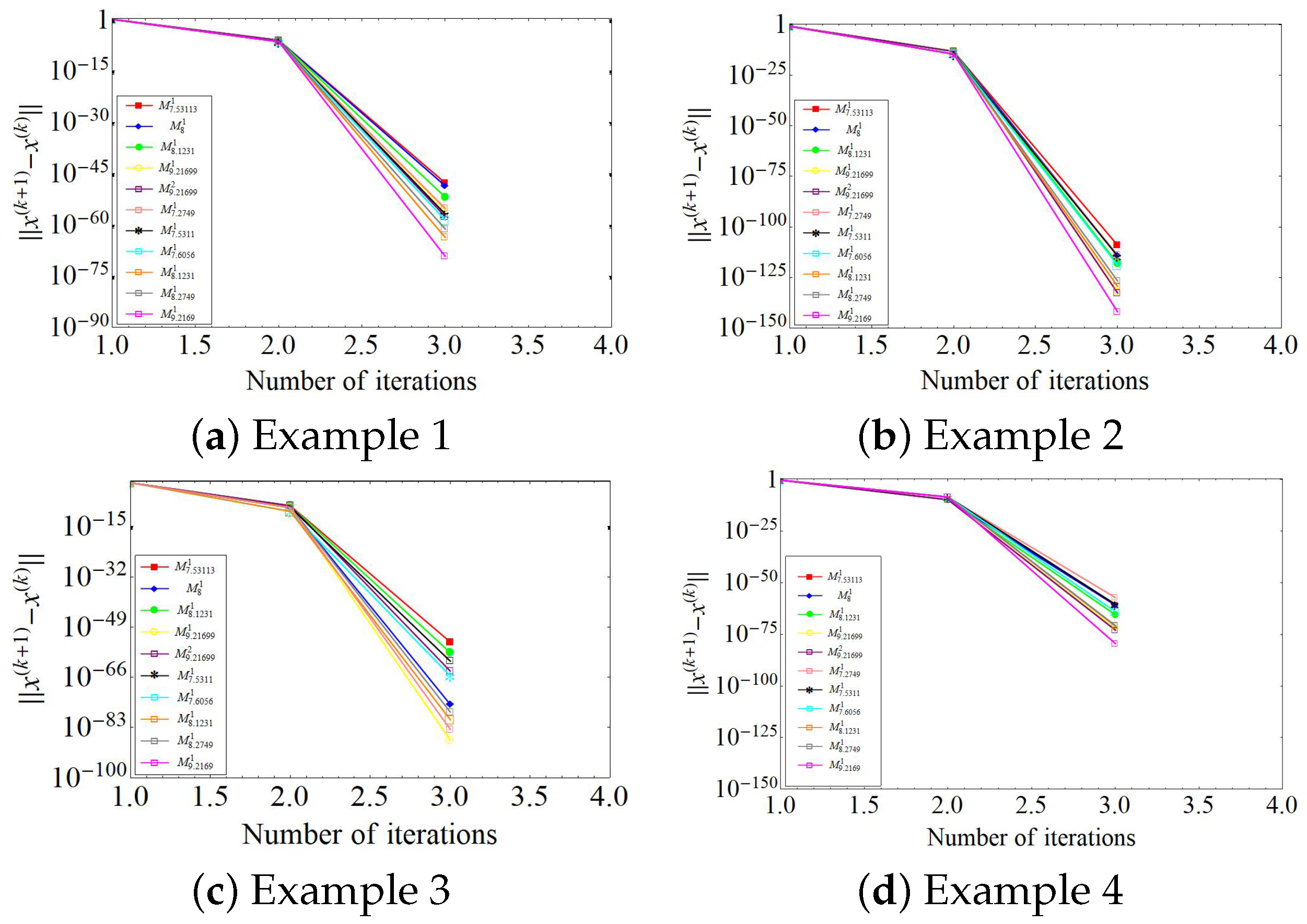
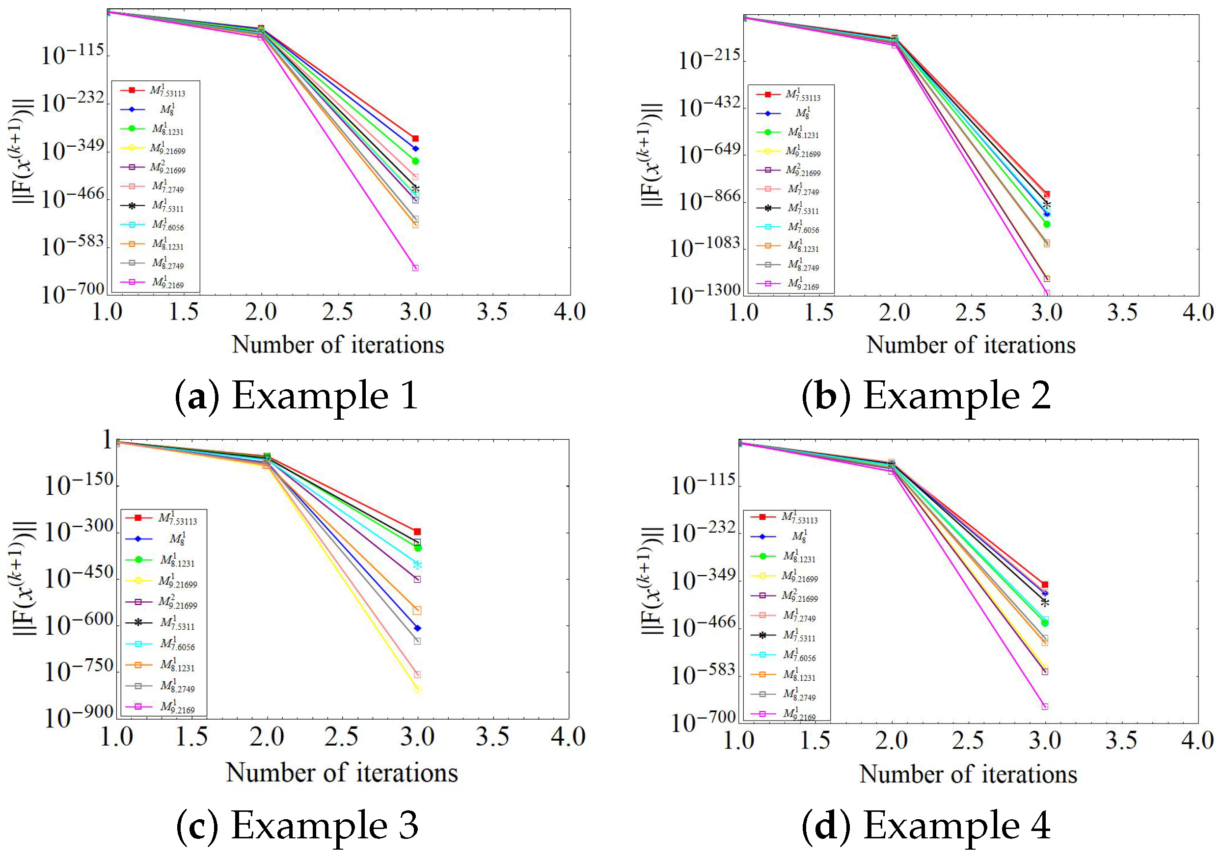
4. Numerical Results and Discussion

In this section, we provide many numerical problems that demonstrate the convergence characteristic of the suggested approaches. The performance of our approach is compared with existing methods, namely $M_{7.53113}^1$, $M_8^1$, $M_{8.12310}^1$, $M_{9.21699}^1$, and $M_{9.21699}^2$, as detailed in reference [2]. All computations were performed using Mathematica 8.0 [19] with multiple-precision arithmetic set to 2048 digits to ensure a high level of accuracy. The stopping criterion for the experiments is the following:

$$\parallel r^{(k+1)}-r^{\left(k\right)}\parallel \le T,$$

where T is the tolerance specific to each method. For each example, the error tolerance is set to $T={10}^{-50}$.

Evaluation Metrics

Table 1, Table 2, Table 3 and Table 4 summarize the numerical results of the compared methods across test examples, using the following metrics:

Table 1. Numerical results for Example 1.

Method	$\mathbf{\left|}\mathbf{\right|}{\mathbf{r}}^{\mathbf{(}\mathbf{k}\mathbf{+}1\mathbf{)}}\mathbf{-}{\mathbf{r}}^{\mathbf{\left(}\mathbf{k}\mathbf{\right)}}\mathbf{\left|}\mathbf{\right|}$	$\mathbf{\left|}\mathbf{\right|}\mathbf{G}\mathbf{\left(}{\mathbf{r}}^{\mathbf{(}\mathbf{k}\mathbf{+}\mathbf{1}\mathbf{)}}\mathbf{\right)}\mathbf{\left|}\mathbf{\right|}$	Iteration	ACOC	CPU
$M_{7.53113}^1$	$1.69\times {10}^{-318}$	$3.49\times {10}^{-2065}$	4	6.4713	0.12497
$M_8^1$	$2.36\times {10}^{-343}$	$5.41\times {10}^{-2362}$	4	6.9013	0.12497
$M_{8.12310}^1$	$1.35\times {10}^{-52}$	$1.57\times {10}^{-373}$	3	7.4977	0.10935
$M_{9.21699}^1$	$2.05\times {10}^{-56}$	$2.85\times {10}^{-454}$	3	8.1214	0.09372
$M_{9.21699}^2$	$2.70\times {10}^{-58}$	$3.91\times {10}^{-469}$	3	8.4288	0.09376
$M_{7.2749}^1$	$6.46\times {10}^{-56}$	$2.44\times {10}^{-411}$	3	7.2829	0.07820
$M_{7.5311}^1$	$1.51\times {10}^{-57}$	$3.02\times {10}^{-436}$	3	7.5839	0.09369
$M_{7.6056}^1$	$2.52\times {10}^{-59}$	$1.84\times {10}^{-456}$	3	7.6127	0.09372
$M_{8.1231}^1$	$2.07\times {10}^{-64}$	$2.87\times {10}^{-529}$	3	8.1148	0.09372
$M_{8.2749}^1$	$6.18\times {10}^{-62}$	$7.70\times {10}^{-515}$	3	8.2785	0.09371
$M_{9.2169}^1$	$6.32\times {10}^{-70}$	$6.68\times {10}^{-635}$	3	9.0000	0.07810

Table 2. Numerical results for Example 2.

Method	$\mathbf{\left|}\mathbf{\right|}{\mathbf{r}}^{\mathbf{(}\mathbf{k}\mathbf{+}\mathbf{1}\mathbf{)}}\mathbf{-}{\mathbf{r}}^{\mathbf{\left(}\mathbf{k}\mathbf{\right)}}\mathbf{\left|}\mathbf{\right|}$	$\mathbf{\left|}\mathbf{\right|}\mathbf{G}\mathbf{\left(}{\mathbf{r}}^{\mathbf{(}\mathbf{k}\mathbf{+}\mathbf{1}\mathbf{)}}\mathbf{\right)}\mathbf{\left|}\mathbf{\right|}$	Iteration	ACOC	CPU
$M_{7.53113}^1$	$1.02\times {10}^{-109}$	$1.08\times {10}^{-829}$	3	7.7019	1.62081
$M_8^1$	$6.57\times {10}^{-115}$	$4.47\times {10}^{-922}$	3	8.1189	1.44667
$M_{8.12310}^1$	$7.19\times {10}^{-119}$	$1.71\times {10}^{-970}$	3	8.4372	1.70871
$M_{9.21699}^1$	$6.44\times {10}^{-133}$	$2.79\times {10}^{-1217}$	3	9.5661	1.55475
$M_{9.21699}^2$	$2.31\times {10}^{-133}$	$2.95\times {10}^{-1222}$	3	9.6019	1.58814
$M_{7.2749}^1$	$1.40\times {10}^{-114}$	$1.42\times {10}^{-837}$	3	7.2153	1.35980
$M_{7.5311}^1$	$4.64\times {10}^{-115}$	$1.30\times {10}^{-871}$	3	7.2502	1.23408
$M_{7.6056}^1$	$1.08\times {10}^{-119}$	$2.20\times {10}^{-914}$	3	7.5866	1.32781
$M_{8.1231}^1$	$4.60\times {10}^{-130}$	$2.27\times {10}^{-1061}$	3	8.3395	1.32781
$M_{8.2749}^1$	$2.21\times {10}^{-127}$	$2.72\times {10}^{-1055}$	3	8.1448	1.32781
$M_{9.2169}^1$	$1.10\times {10}^{-142}$	$2.86\times {10}^{-1289}$	3	9.2559	1.32781

Table 3. Numerical results for Example 3.

Method	$\left|\right|{\mathbf{r}}^{(\mathbf{k}+1)}-{\mathbf{r}}^{\left(\mathbf{k}\right)}\left|\right|$	$\left|\right|\mathbf{G}\left({\mathbf{r}}^{(\mathbf{k}+1)}\right)\left|\right|$	Iteration	ACOC	CPU
$M_{7.53113}^1$	$9.22\times {10}^{-55}$	$2.15\times {10}^{-298}$	3	5.9409	96.67874
$M_8^1$	$6.68\times {10}^{-76}$	$5.04\times {10}^{-609}$	3	7.8965	95.12069
$M_{8.12310}^1$	$2.37\times {10}^{-58}$	$8.82\times {10}^{-350}$	3	6.4033	105.39603
$M_{9.21699}^1$	$5.09\times {10}^{-88}$	$1.55\times {10}^{-806}$	3	9.3335	102.83968
$M_{9.21699}^2$	$1.26\times {10}^{-64}$	$1.03\times {10}^{-452}$	3	7.2114	83.71736
$M_{7.5311}^1$	$3.00\times {10}^{-61}$	$3.02\times {10}^{-332}$	3	6.2215	80.48735
$M_{7.6056}^1$	$3.22\times {10}^{-66}$	$6.50\times {10}^{-401}$	3	5.7464	96.65305
$M_{8.1231}^1$	$4.37\times {10}^{-81}$	$2.24\times {10}^{-551}$	3	7.2814	87.39948
$M_{8.2749}^1$	$1.79\times {10}^{-78}$	$2.19\times {10}^{-651}$	3	8.2819	93.83893
$M_{9.2169}^1$	$2.43\times {10}^{-84}$	$9.32\times {10}^{-760}$	3	8.9837	93.94005

Table 4. Numerical results for Example 4.

Method	$\left|\right|{\mathbf{r}}^{(\mathbf{k}+1)}-{\mathbf{r}}^{\left(\mathbf{k}\right)}\left|\right|$	$\left|\right|\mathbf{G}\left({\mathbf{r}}^{(\mathbf{k}+1)}\right)\left|\right|$	Iteration	ACOC	CPU
$M_{7.53113}^1$	$1.47\times {10}^{-61}$	$3.24\times {10}^{-359}$	3	5.3853	0.07810
$M_8^1$	$1.31\times {10}^{-61}$	$1.08\times {10}^{-380}$	3	5.3905	0.07810
$M_{8.12310}^1$	$3.34\times {10}^{-66}$	$8.01\times {10}^{-453}$	3	5.8755	0.07806
$M_{9.21699}^1$	$5.31\times {10}^{-73}$	$2.40\times {10}^{-563}$	3	6.5931	0.10935
$M_{9.21699}^2$	$1.09\times {10}^{-73}$	$2.17\times {10}^{-573}$	3	6.6658	0.10934
$M_{7.2749}^1$	$5.86\times {10}^{-58}$	$1.96\times {10}^{-377}$	3	5.9520	0.07807
$M_{7.5311}^1$	$3.46\times {10}^{-61}$	$1.29\times {10}^{-399}$	3	6.3465	0.07814
$M_{7.6056}^1$	$1.14\times {10}^{-64}$	$5.04\times {10}^{-495}$	3	6.7772	0.07814
$M_{8.1231}^1$	$9.41\times {10}^{-72}$	$1.56\times {10}^{-502}$	3	7.6376	0.07807
$M_{8.2749}^1$	$1.81\times {10}^{-71}$	$6.71\times {10}^{-491}$	3	7.6028	0.06245
$M_{9.2169}^1$	$3.47\times {10}^{-80}$	$3.56\times {10}^{-660}$	3	8.6682	0.10934

• The computed approximation ($r^{(k+1)}$).
• The function value ($\parallel G\left(r^{(k+1)}\right)\parallel$).
• Distance between consecutive iterations, ($\parallel r^{(k+1)}-r^{\left(k\right)}\parallel$).
• Iteration count required to satisfy the stopping criteria.
• The approximated computational order of convergence (ACOC):

  $$ACOC\sim {\displaystyle \frac{log\left(\frac{\parallel r^{(k+1)}-r^{\left(k\right)}\parallel }{\parallel r^{\left(k\right)}-r^{(k-1)}\parallel }\right)}{log\left(\frac{\parallel r^{\left(k\right)}-r^{(k-1)}\parallel }{\parallel r^{(k-1)}-r^{(k-2)}\parallel }\right)}}.$$
• The total CPU time taken for the entire computation process.

These metrics provide a comprehensive comparison of the efficiency, accuracy, and convergence speed of the proposed techniques relative to existing schemes.

Example 1.

We consider the boundary value problem specified below (see [9]):

$$y^{″}={\displaystyle \frac{1}{2}}{y}^3+3y^{\prime }-{\displaystyle \frac{3}{2-x}}+{\displaystyle \frac{1}{2}};y\left(0\right)=0,y\left(1\right)=1.$$

Consider dividing the interval $[0,1]$ as

$$x_0=0<x_1<x_2<\dots <x_{n-1}<x_n=1,x_{i+1}=x_i+h,h={\displaystyle \frac{1}{n}}.$$

Define the discrete variables corresponding to the function values at the partition points:

$$y_0=y\left(x_0\right),y_1=y\left(x_1\right),\dots ,y_{n-1}=y\left(x_{n-1}\right),y_n=y\left(x_n\right).$$

Using numerical approximations for the first and second derivatives, we obtain the following:

$$\begin{array}{cc}\hfill y_k^{\prime }& \approx {\displaystyle \frac{y_{k+1}-y_{k-1}}{2h}},k=1,2,3,\dots ,n-1,\hfill \\ \hfill y_k^{″}& \approx {\displaystyle \frac{y_{k-1}-2y_k+y_{k+1}}{h^2}},k=1,2,3,\dots ,n-1.\hfill \end{array}$$

By substituting these approximations into the governing equation, we obtain a set of $(n-1)$ nonlinear equations for $(n-1)$ variables:

$$y_{k+1}-2y_k+y_{k-1}-{\displaystyle \frac{h^2}{2}}{y}_k^3-{\displaystyle \frac{3}{2}}h(y_{k+1}-y_{k-1})+{\displaystyle \frac{3}{2-x_k}}{h}^2-{\displaystyle \frac{1}{2}}{h}^2=0,k=1,2,3,\dots ,n-1.$$

• Specific Case:  $n=5$

For $n=5$, the step size and partition points are as follows:

$$h={\displaystyle \frac{1}{5}},x_k=kh,k=0,1,2,3,4,5.$$

The initial values are set as follows:

$$y^{\left(0\right)}=\left[\begin{array}{c}1\\ 1\\ 1\\ 1\end{array}\right],t^{\left(0\right)}=-0.01I,$$

where the identity matrix is indicated by I.

Example 2.

Now, consider the system of six equations as described in ref. [20]:

$$\sum _{j=1,j\ne i}^6{x}_j-e^{-x_i}=0,1\le i\le 6,$$

With an initial guess $r^{\left(0\right)}={\{0.25,0.25,0.25,0.25,0.25,0.25\}}^T$ and initializing $t^{\left(k\right)}$ with $t^{\left(0\right)}=-0.01I$, where the identity matrix is denoted by I, the error tolerance is set to ${10}^{-50}$.

Example 3.

We examine the fifty-equation system: (taken from [2]):

$$\begin{array}{cc}\hfill x_i^2{x}_{i+1}-1& =0,1\le i\le 49,\hfill \\ \hfill x_{50}^2{x}_1-1& =0.\hfill \end{array}$$

The tolerance for this example is ${10}^{-50}$, the starting guess is $r^{\left(0\right)}={\left\{0.9,0.9,\dots ,0.9\right\}}^T$, and the initial estimates for the vectors $r^{(-1)}$, $p^{(-1)}$, and $q^{(-1)}$ are ${\left\{0.7,0.7,\dots ,0.7\right\}}^T$.

Example 4.

We examine the three-equation system: (adapted from [6]):

$$\begin{array}{cc}\hfill 10x+sin(x+y)-1& =0,\hfill \\ \hfill 8y-{cos}^2(z-y)-1& =0.\hfill \\ \hfill 12z+sinz-1& =0.\hfill \end{array}$$

The tolerance for this example is ${10}^{-50}$, the starting guess is $r^{\left(0\right)}={\left\{0.5,0.1,0.1\right\}}^T$. The parameter $t^{\left(k\right)}$ is initialized as $t^{\left(0\right)}=-0.01I$, where I represents the identity matrix.

Figure 2 provides a graphical representation of the errors at each consecutive iteration for the different iterative processes employed to solve Examples 1–4. The figure highlights the superior performance of our proposed method (15)–(17) compared to other well-known methods. Specifically, it shows that our method converges more rapidly and achieves significantly higher computational accuracy across all examples.

Figure 2. Graphical comparison of errors in consecutive iteration for Examples 1–4.

Furthermore, Figure 3 depicts the function values at each iteration for Examples 1–4. These results reaffirm the effectiveness of our approach in achieving consistent and accurate solutions while maintaining stability in the iterative process. The function values obtained using our method exhibit a faster decrease to zero (or the desired tolerance), which is a direct indicator of superior convergence characteristics.

Figure 3. The graphical comparison illustrates the values of the functions at each iteration for Examples 1–4.

In addition to accuracy, computational efficiency is a critical aspect when comparing iterative methods. For the four examples considered, our method demonstrates a notable reduction in CPU time compared to other existing methods. This computational advantage arises from the robust design of our iterative scheme, which effectively reduces the number of iterations required to achieve the desired tolerance. Consequently, our approach is not only more accurate but also computationally efficient, making it a preferable choice for solving nonlinear systems.

These results collectively highlight the advantages of our proposed method in terms of both computational accuracy and efficiency, particularly when compared to other well-established methods from the literature.

5. Conclusions

We have developed a new family of three-step derivative-free iterative algorithms with memory for solving a system of nonlinear equations. Using the first-order divided difference operator for multivariable functions and applying Taylor expansion, we have determined the minimal order of convergence for these techniques. The convergence orders were determined to be $7.2749$, $7.5311$, $7.6056$, $8.1231$, $8.2749$ and $9.2169$. To enhance the convergence speed, we incorporated a self-accelerating parameter that evolves as the iterations progress, which is implemented through a self-correcting matrix. This allows for faster convergence in solving nonlinear equation systems. Furthermore, we have evaluated the computational efficiency of our schemes against existing approaches, with numerical experiments demonstrating that our methods achieve significantly better performance. These findings validate the effectiveness and reliability of our proposed approach. In future research, this technique will be extended to similar methods [4,5,6,8,20].

References

- Steffensen, J. Remarks on iteration. Scand. Actuar. J. 1993, 1, 64–72. [Google Scholar] [CrossRef]
- Cordero, A.; Garrido, N.; Torregrosa, J.R.; Triguero, P.N. Design of iterative methods with memory for solving nonlinear systems. Math. Methods Appl. Sci. 2023, 46, 12361–12377. [Google Scholar] [CrossRef]
- Chicharro, F.I.; Cordero, A.; Garrido, N.; Torregrosa, J.R. On the improvement of the order of convergence of iterative methods for solving nonlinear systems by means of memory. Appl. Math. Lett. 2020, 104, 106277. [Google Scholar] [CrossRef]
- Cordero, A.; Garrido, N.; Torregrosa, J.R.; Triguero, P.N. Improving the order of a fifth-order family of vectorial fixed point schemes by introducing memory. Fixed Point Theory J. 2023, 24, 155–172. [Google Scholar] [CrossRef]
- Behel, R.; Cordero, A.; Torregrosa, J.R.; Bhalla, S. A new high-order jacobian-free iterative method with memory for solving nonlinear system. Mathematics 2021, 9, 2122. [Google Scholar] [CrossRef]
- Petkovic, M.S.; Sharma, J.R. On some efficient derivative-free iterative methods with memory for solving systems of nonlinear equations. Numer. Algorithms 2016, 71, 457–474. [Google Scholar] [CrossRef]
- Argyros, I.K. The Theory and Applications of Iteration Methods, 2nd ed.; Engineering Series; CRC Press—Taylor and Francis Corp.: Boca Raton, FL, USA, 2022. [Google Scholar]
- Sharma, J.R.; Arora, H. A novel derivative free algorithm with seventh order convergence for solving systems of nonlinear equations. Numer. Algorithms 2014, 67, 917–933. [Google Scholar] [CrossRef]
- Ortega, J.M.; Rheinboldt, W.C. Iterative Solution of Nonlinear Equations in Several Variables; SIAM: Philadelphia, PA, USA, 2000. [Google Scholar]
- Kurchatov, V.A. On a method of linear interpolation for the solution of functional equations. Dokl. Akad. Nauk. SSSR 1971, 198, 524–526. [Google Scholar]
- Shakhno, S.M. On a Kurchatov’s method of linear interpolation for solving nonlinear equations. PAAM-Proc. Appl. Math. Mech. 2004, 4, 650–651. [Google Scholar] [CrossRef]
- Shakhno, S.M. On the difference method with quadratic convergence for solving nonlinear operator equations. Mat. Stud. 2006, 26, 105–110. [Google Scholar]
- Ezquerro, J.A.; Grau, A.; Grau-Sanchez, M.; Hernandez, M. On the efficiency of two variants of Kurchatov’s method for solving nonlinear systems. Numer. Algorithms 2013, 64, 685–698. [Google Scholar] [CrossRef]
- Argyros, I.K. Advances in the Efficiency of Computational Methods and Applications; World Scientific Publishing Company: Singapore, 2000. [Google Scholar]
- Grau-Sánchez, M.; Grau, Á.; Noguera, M. Ostrowski type methods for solving systems of nonlinear equations. Appl. Math. Comput. 2011, 218, 2377–2385. [Google Scholar] [CrossRef]
- Grau-Sánchez, M.; Noguera, M. A technique to choose the most efficient method between secant method and some variants. Appl. Math. Comput. 2012, 218, 6415–6426. [Google Scholar] [CrossRef]
- Grau-Sánchez, M.; Grau, Á.; Noguera, M. Frozen divided difference scheme for solving systems of nonlinear equations. J. Comput. Appl. Math. 2011, 235, 1739–1743. [Google Scholar] [CrossRef]
- Grau-Sánchez, M.; Noguera, M.; Amat, S. On the approximation of derivatives using divided difference operators preserving the local convergence order of iterative methods. J. Comput. Appl. Math. 2013, 237, 363–372. [Google Scholar] [CrossRef]
- Wolfram, S. The Mathematica Book; Wolfram Research, Inc.: Champaign, IL, USA, 2003. [Google Scholar]
- Sharma, J.R.; Arora, H. An efficient derivative free iterative method for solving systems of nonlinear equations. Appl. Anal. Discret. Math. 2013, 141, 390–403. [Google Scholar] [CrossRef]
Disclaimer/Publisher’s Note: The statements, opinions and data contained in all publications are solely those of the individual author(s) and contributor(s) and not of MDPI and/or the editor(s). MDPI and/or the editor(s) disclaim responsibility for any injury to people or property resulting from any ideas, methods, instructions or products referred to in the content. |
© 2025 by the authors. Licensee MDPI, Basel, Switzerland. This article is an open access article distributed under the terms and conditions of the Creative Commons Attribution (CC BY) license (https://creativecommons.org/licenses/by/4.0/).