Article

Blind Source Separation Using Time-Delayed Dynamic Mode Decomposition

by
Gyurhan Nedzhibov
Faculty of Mathematics and Informatics, Shumen University, 9700 Shumen, Bulgaria
Computation 2025, 13(2), 31; https://doi.org/10.3390/computation13020031
Submission received: 18 December 2024 / Revised: 19 January 2025 / Accepted: 22 January 2025 / Published: 1 February 2025
(This article belongs to the Special Issue Mathematical Modeling and Study of Nonlinear Dynamic Processes)

Abstract

:
Blind Source Separation (BSS) is a significant field of study in signal processing, with many applications in various fields such as audio processing, speech recognition, biomedical signal analysis, image processing and communication systems. Traditional methods, such as Independent Component Analysis (ICA), often rely on statistical independence assumptions, which may limit their performance in systems with significant temporal dynamics. This paper introduces an extension of the dynamic mode decomposition (DMD) approach by using time-delayed coordinates to implement BSS. Time-delay embedding enhances the capability of the method to handle complex, nonstationary signals by incorporating their temporal dependencies. We validate the approach through numerical experiments and applications, including audio signal separation, image separation and EEG artifact removal. The results demonstrate that modification achieves superior performance compared to conventional techniques, particularly in scenarios where sources exhibit dynamic coupling or non-stationary behavior.

1. Introduction

Although machine learning and neural networks dominate many aspects of data science and signal processing, deterministic, interpretable signal processing tools are still of great interest. One such method is Blind Source Separation (BSS), introduced around 1984 within the framework of neural modeling  [1,2].
It is a computational method that extracts individual source signals from mixed observations without any knowledge of the sources or the mixing process. The ability to disentangle mixed signals into their underlying components is critical for enhancing the quality of data analysis, facilitating feature extraction, and enabling downstream applications such as pattern recognition and anomaly detection. When unintentionally mixed signals are present due to environmental conditions or undesirable signals, BSS is one of the best approaches for separating the signals. The BSS approach has attracted significant attention due to its applicability in a wide range of fields including signal and image processing [3,4], communication technologies  [5], biomedical data analysis [6,7], neural networks [8], human brain activity [9], audio signal recovery [10], cocktail party problem, and telecommunications [11,12,13]. BSS has potential for application in fields such as industrial applications, for signal separation in radar systems [14] and synthetic aperture radar (SAR) image processing [15]; in astronomy and astrophysics, for gravitational-wave signals analysis [16] and research into the earth’s magnetic field [17].
Some of the traditional methods for solving BSS problem are:
  • Independent Component Analysis (ICA) [18], which relies on statistical independence between sources. One of the most popular algorithms for performing ICA is FastICA  [19].
  • Principal Component Analysis (PCA) [20], which uses correlation between signals to reduce the dimensionality of the problem.
  • Non-negative Matrix Factorization (NMF) [21], which is useful in analyzing signals such as audio and images when the data is nonnegative.
They are widely used in a broad range of possible applications, but suffer from limitations related to assumptions of independence or linearity of sources, as well as weaknesses in dynamic and nonlinear systems. Some of the disadvantages of these methods are: ICA may prove invalid in many practical cases, especially when the sources have dynamic dependencies or noise is present, NMF requires only non-negative values or values with specific constraints, PCA does not guarantee a physical or statistical interpretation of the sources.
Besides, the traditional methods do not effectively deal with signals whose components have significant temporal dependencies. These limitations motivate the investigation of new methods that can handle complex dependencies and exploit the dynamic information in the signals. Recently, new approaches have emerged to further enhance the capabilities of BSS. One such method is Convolutional Independent Component Analysis (Conv-ICA) [22], which extends traditional ICA by incorporating convolutional structures, enabling the separation of sources with temporal dependencies. Dynamic Mode Decomposition (DMD)-based BSS  [23] is another advanced technique, which leverages the temporal coherence of signals to identify and separate components in dynamical systems. Additionally, Non-Negative Tensor Factorization (NTF) [24] has been employed to handle multi-dimensional datasets by exploiting non-negativity constraints, making it highly effective for applications in hyperspectral imaging, video analysis, and neuroscience. Another representative of BSS methods is the second-order blind identification (SOBI) algorithm [25], which exploits the temporal coherence of the source signals to obtain its unique set of advantages. However, recent advances in machine learning have led to the development of more sophisticated and versatile models  [26,27,28]. These methods represent a shift toward more flexible, scalable, and application-specific implementations of BSS, addressing limitations of traditional techniques.
Moreover, to extract reliable and meaningful components from the data, pre- and post-processing techniques are also essential  [29]. For example, the most common preprocessing steps for ICA algorithms are centering and whitening. The centering step aims to center signals by subtracting the mean values from signal data. Given an observed vector signal denoted by x , centered observed vector x ¯ can be obtained by x ¯ = x μ , where μ is the mean value, see [30]. The whitening step aims to transform the signal data into uncorrelated components and rescale them by unit variance [31]. It is known that for a whitened x ^ vector, the associated covariance matrix is equal to the identity matrix, i.e., E { x ^ x ^ T } = I .
One way to perform a whitening transformation is to use the eigenvalue decomposition of the covariance matrix E { x x T } = V D V T , where V is a matrix of eigenvectors and D is the diagonal matrix of eigenvalues of the covariance matrix. The observed vector can be whitened by the following transformation [19]: x ^ = V D 1 / 2 V T x can whiten the observed vector, where D 1 / 2 = diag { d i 1 / 2 } . After the transformation, x ^ = V D 1 / 2 V T A s = A ^ s holds, which leads to E { x ^ x ^ T } = A ^ E { s s T } A ^ T = A ^ A ^ T = I , see also [32].
In this paper, we investigate the application of the dynamic mode decomposition (DMD) approach [33] to solve the BSS problem. DMD is a relatively new method developed for the analysis of dynamical systems. It extracts the dynamic modes of the system, which represent the fundamental frequency and spatial characteristics of the signals. This makes it a powerful tool for the analysis of time series and nonlinear systems represented in linear form. The application of standard forms of the DMD approach to demixing ergodic time series and Fourier series is presented in  [23,34,35] and the demixing of chaotic signals and images is discussed in [36]. n the remainder of this section, the frameworks of the BSS and DMD methods will be briefly described.

1.1. The BSS Framework

The BSS problem consists of extracting unobserved sources, denoted in vector notation as s k R p , assuming zero mean and stationary from observations or measurements x k R m , which can be written:
x k = Q s k
where Q : R p R m is an unknown mapping and k denotes the sample index, which can denote time for example.
Let us assume, we are given n observed samples x 1 , , x n corresponding to uniformly spaced time instances t 1 , , t n , i.e.,
x i = x ( t i ) = [ x 1 ( t i ) , , x m ( t i ) ] T and s i = s ( t i ) = [ s 1 ( t i ) , , s p ( t i ) ] T
for i = 1 , , n . If the mapping A is restricted to a simple matrix, then the model (1) can also be written in matrix form as:
X = Q S ,
where X = [ x 1 , , x n ] and S = [ s 1 , , s n ] . This is the noiseless case of BSS model for instantaneous linear mixtures.
The main idea of BSS is to recover the original signals S from the observed mixtures X. If the matrix Q is invertible, then usually the condition m p is required. Determining Q or its inverse W, directly leads to source separation, i.e., provides estimated sources such that:
S ^ = W X .
In this case, the sources are evaluated up to a permutation and scale.
If the number of sources p is greater than the number of observations m, the mixing is called underdetermined and is not reversible. In this case, even if the mixing matrix is completely known, there is an infinity of solutions and additional constraints required to restore the essential uniqueness of the source inputs.
A problem characterized by a model like (2) would certainly be ill-posed if additional assumptions were not made about the characteristics of the system. These hypotheses can be divided into two groups, depending on whether they are related to the mixing matrix or the sources. The basic BSS methods rely on the following:
  • The number of observations is greater than the number of sources ( m p ) and the mixing matrix Q is of full column rank.
  • Each row-vector of S is a stationary stochastic process with zero mean.
  • The unknown sources are statistically independent (at each instant t, the components of S ( t ) are mutually statistically independent).
Equation (2) reveals that the matrix X is a linear combination of rows of the latent matrix S.

1.2. The DMD Framework

First, we give a description of the standard DMD algorithm. Let us consider a sequential data set
D = { x 1 , x 2 , , x n } ,
where each x k R m . Assume that the data are uniformly distributed in time and the collection time varies from t 1 to t n . The main assumption of the method is that there exists a linear (unknown) operator A connecting x k to the subsequent x k + 1 :
x k + 1 = A x k
for k = 1 , , n 1 . The eigenvalues of A contain information about the growth or decay rates and the frequencies of oscillations, which, when combined, represent the time evolution of the dynamical system. The DMD method uses the arrangement of the data set D into following two matrices:
X = [ x 1 , , x n 1 ] and Y = [ x 2 , , x n ] ,
and the dependence (5) has an equivalent matrix form
Y = A X .
Then the dynamic mode decomposition of data matrix D is given by the eigendecomposition of A. DMD finds the best-fit solution A that minimizes the least-squares distance in the Frobenius norm
arg min A Y A X F ,
where . F is the Frobenius norm. The solution A to this optimization problem is given by
A = Y X ,
where X is a Moore-Penrose pseudo-inverse of X. Having a spectral decomposition of A, we can reconstruct data matrix D . Let ϕ i and λ i denote the i-th pair of eigenvectors and eigenvalues of A, respectively, for  i = 1 , , m . Therefore, the following expression is valid  [37]:
D = Φ B V ( λ ) ,
where Φ is the eigenvector matrix (with columns ϕ i ) and V ( λ ) = ( v i j ) is a Vandermonde matrix such that v i j = λ i j 1 for i = 1 , , m and j = 2 , , n . In Equation (9) B is a diagonal matrix B = diag { b i } , with diagonal elements, the components of the initial amplitude vector b = Φ x 1 .
There are many conceptually equivalent but mathematically different definitions of DMD. A more general definition of the described method is presented by Tu et al. in [38], where the data is collected as a set of snapshot pairs
{ ( x j , y j ) } j = 1 n 1
instead of sequential time series. In (10), the vectors x j , y j R m are spaced a fixed time interval apart. Then the two sets of data corresponding to (6) are:
X = [ x 1 , , x n 1 ] and Y = [ y 1 , , y n 1 ] ,
The dynamic mode decomposition of the data pair ( X , Y ) is given by the eigendecomposition of the best fit linear operator A such that
Y = A X .
The eigenvectors and eigenvalues of the matrix A are the DMD modes and eigenvalues. Note that the formulation (6) and (7) is a special case of (11) and (12), with  y k = x k + 1 for k = 1 , , n 1 . The DMD approach described is known as exact DMD.

Reduced Order DMD Operator

In practice, the matrix A can be very high dimensional, and calculating its eigendecomposition can be very expensive. The main goal of DMD is to compute the leading eigendecomposition of A without explicitly representing or manipulating A. For this purpose, a low-rank approximation matrix A is constructed and its eigendecomposition is calculated to obtain the DMD modes and eigenvalues.
Usually, the projection matrix of A is performed onto the subspace spanned by the columns of X. Let the reduced singular value decomposition of X be:
X = U r Σ r V r * ,
where U r R m × r , Σ r R m × r , V r R n × r and r = rank ( X ) . We can derive the projection operator as
A ˜ = U r * A U r = U r * Y V r Σ r 1 ,
such that its eigenvalues are also the eigenvalues of A. Therefore, from the spectral decomposition of A ˜
A ˜ W = W Λ ,
where Λ = diag { λ j } j = 1 r is the matrix of eigenvalues and W is the matrix of eigenvectors of A ˜ , we determine the leading eigendecomposition of A. The matrix of DMD modes is computed by the formula
Φ r = Y V r Σ r 1 W .
The columns of matrix Φ r R m × r are often called exact DMD modes, because Tu et al. [38] prove that these are exact eigenvectors of matrix A. In this case we extract r leading eigenvectors of A. This approach is known as SVD based DMD.

1.3. BSS in Context of DMD

Dynamic Mode Decomposition can provide a framework for realizing Blind Source Separation by leveraging the decomposition of a dynamic system into modes and temporal dynamics. In the context of BSS, the observed data matrix X ( t ) is modeled as X ( t ) = Q S ( t ) , where Q is the mixing matrix and S ( t ) contains the independent source signals. When Q is square ( m = p , i.e., the number of observed signals is equal to the number of sources), DMD can directly approximate Q by the DMD mode matrix Φ and S ( t ) can be reconstructed using the Vandermonde structure of the DMD eigenvalues. In overdetermined cases ( m > p ), Φ still captures the dominant dynamics, but disentangling Q and S ( t ) requires careful dimensionality reduction or augmentation. Conversely, in underdetermined cases ( m < p ), DMD alone cannot resolve the sources and additional constraints or methods, such as time delay embedding, are needed. The success of DMD-based BSS also depends on the statistical independence of S ( t ) and the full rank of Q. Deviations from these assumptions can challenge the separation, but can often be mitigated by augmenting the data or regularizing the decomposition. Overall, DMD offers a powerful and interpretable approach to BSS, adaptable to different system configurations.
Some studies dedicated to the idea of applying the DMD method to solve the BSS problem are the following: Hirsh et al. in  [39] consider the case that all modes s j are intrinsic mode functions (IMF) with interwave frequency modulation; Prasadan et al. in [23] investigate the case of uncorrelated latent time series with lag one that have nonzero autocorrelation, and in [35] an extension to time series uncorrelated at higher lag times is introduced, see also [36].
It should be noted that all of these applications of the DMD method to implement BSS use the exact DMD approach described in Section 1.2. While in [23] a lag one time series is used (i.e., the scheme described in (6)–(9)), in [35,36] the idea of a higher order lag times is considered, corresponding to that described in (10)–(12). This in turn implies that the computed mixing matrix Φ , in (9), is a square matrix, i.e., the approach is applicable only in cases where the number of observable signals is equal to the number of sources, m = p .
In this study, we will extend the idea of applying DMD to BSS implementation by using the svd-based DMD approach described in (13)–(15), so that the method is applicable to the overdetermined case as well. Furthermore, we will generalize this concept to use time-delay coordinates to expand the application range of the proposed scheme. In the next section, we will describe the idea of using time delays in the DMD approach, and after that in Section 3, we will present the TD-DMD implementation scheme for BSS.

2. Time-Delayed DMD

Time-Delayed DMD (TD-DMD) is an extension of standard DMD that incorporates time delays in the data to capture more complex dynamic information. This approach overcomes several shortcomings of the standard DMD method by extending its capabilities to handle long-term temporal behavior, nonlinear dynamics, nonuniformly sampled data, high-dimensional datasets, and noisy data. This makes it a more versatile and robust technique for dynamic mode decomposition in various applications. The approach is based on the Takens embedding theorem [40], which provides a rigorous framework for analyzing the information content of measurements of a nonlinear dynamical system. The scheme of delay-embedded DMD consists of the following: given the data sequence D in (4), we arrange s time-shifted copies of the data to form an augmented input matrix. The following Hankel matrix is formed:
D a u g = x 1 x 2 x m s + 1 x 2 x 3 x m s + 2 x s x s + 1 x m ,
where s is the delay embedding dimension. The augmented data matrix D a u g is then used instead of D and processed by the core DMD algorithm.
This increases the dimensionality of space and provides additional information about time dependencies. Applying DMD to this extended matrix allows the extraction of modes that are better adapted to complex temporal structures.

2.1. Hankel DMD

The DMD approach described in the previous paragraph is applied to augmented data matrices:
X a u g = x 1 x m s x 2 x m s + 1 x s x m 1 and Y a u g = x 2 x m s + 1 x 3 x m s + 2 x s + 1 x m .
We use matrices X a u g , Y a u g R ( m . s ) × ( n s ) in place of X and Y, giving eigenvalues Φ a u g and modes Λ a u g . The first m rows of Φ a u g correspond to the current-state DMD modes used to reconstruct initial data D . In this case, the DMD operator is expressed as A = Y a u g X a u g , according to (8). The reduced-order DMD operator A ˜ can be calculated by a formula of the form (13), and then the DMD mode matrix by a formula of the form (15). The first m rows of Φ a u g correspond to the DMD modes of the current state used to reconstruct the initial data D .
Among the reasons to compute DMD on these delay coordinates is that if the state measurements are low-dimensional, it may be necessary to increase the rank of the X a u g matrix by using delay coordinates. In general, adding more rows only results in additional singular values of X a u g , hence we may increase the number of delay coordinates s until the system reaches full rank numerically.

2.2. Higher Order DMD

Here we consider the idea of a higher-order extension of the standard DMD that is capable of providing highly accurate results in cases where the performance of the classical DMD deteriorates or even fails. The goal is to mix the classical DMD with the Taken delay embedding theorem [40], leading to the higher-order Koopman conjecture, which uses time-lagged snapshots, such as
x k + s = A 1 x k + A 2 x k + 1 + A s x k + s 1 ,
for k = 1 , , m s .
Let us note that s 1 is adjustable and for s = 1 this assumption coincides exactly with the standard Koopman assumption presented in Equation (5). The resulting mapping is given by
A X a u g = Y a u g ,
where X a u g and Y a u g are defined in (17), and A is a block companion matrix:
A = 0 I 0 0 0 0 I 0 0 0 0 I A 1 A 2 A 3 A s .
with A i R n × n , 0 is the n × n zero matrix and I is the n × n unit matrix. Using the augmented data matrices X a u g and Y a u g and the higher-order Koopman operator A , we can implement the basic DMD algorithm and extract spectral information from temporally broadband or spatially sparse data sequences. The higher-order extension adds more robustness and flexibility to the standard algorithm and allows analysis of systems for which temporal resolution is substituted for spatial resolution.
The described higher-order DMD scheme was introduced by Le Clainche and Vega in [41,42]. However, the algorithm presented there does not exploit the special form of the generalized Koopman matrix A in (20).
What follows is to introduce a more cost-effective way to compute the operator A , as well as an explicit formula for computing the corresponding reduced DMD operator A ˜ . For more details, we refer to  [43].

2.2.1. Cost Effective Calculation of Higher-Order DMD Operator

Let us represent the operator A R s . n × s . n in the following equivalent block matrix form:
A = 0 I A 1 A 2 : s ,
where 0 R ( s 1 ) n × n is the zero matrix, I R ( s 1 ) n × ( s 1 ) n is the identity matrix, A 1 R n × n and A 2 : s R n × ( s 1 ) n is the block matrix A 2 : s = [ A 2 | | A s ] .
Let us now use the following representation for the extended matrices X a u g and Y a u g defined in (17):
X a u g = X 1 X 2 X s and Y a u g = X 2 X 3 X s + 1 ,
where X i R n × ( m s ) has the form
X i = [ x i | x i + 1 | x m s + i 1 ]
for i = 1 , , s + 1 .
From (22) and (23) the equivalent representations follow
X a u g = X 1 X 2 ; s and Y a u g = X 2 ; s X s + 1 ,
where double indexing is used for a matrix of the form:
X p ; q = X p X q .
From (19) the equivalent representations follow:
A X a u g = Y a u g 0 I A 1 A 2 : s X a u g = X 2 ; s X s + 1 .
On the other hand, matrix A is expressed in the following way
A = Y a u g X a u g ,
where X a u g is the Moore-Penrose pseudoinverse of X a u g . From the above two equations it follows that
A = 0 I A 1 A 2 : s = X 2 ; s X s + 1 X a u g .
To calculate the block matrix A it is sufficient to calculate the last row of matrices:
A 1 : s = [ A 1 | A 2 | | A s ] = X s + 1 X a u g ,
which is n × s . n matrix.

2.2.2. Reduced Order Aproximation of Higher-Order DMD Operator

We consider the reduced SVD of X a u g R s . n × ( m s ) :
X a u g = U X Σ X V X *
where U X R s . n × r , V X R m s × r , Σ X R r × r . Let us represent matrix U X in the form of (22)
U X = U 1 U 2 U s ,
with sub-matrices U i R n × r for i = 1 , , s .
Hence, the reduced order DMD operator
A ˜ = U X * A U X
has the following expression:
A ˜ = [ U 1 ; s 1 * | U s * ] 0 I A 1 A 2 : s U 1 U 2 ; s ,
where 0 R ( s 1 ) n × n is the zero matrix, I R ( s 1 ) n × ( s 1 ) n is the identity matrix. Double indexing is used for block sub-matrices U p ; q of the form:
U p ; q = U p U q .
We obtain the following representation from (32), using (28) and (29):
A ˜ = U 1 ; s 1 * U 2 ; s + U s * X s + 1 V x Σ X 1 ,
which is an r × r matrix. Hence, matrix A ˜ in (33) is the reduced-order approximation of A , which is much more cost-effective than the standard HODMD formula.
For some recent results on the subject, we recommend  [44,45,46,47,48,49,50,51,52,53].

3. BSS by Time-Delayed DMD

In this section, we first describe the concept of applying time-delayed DMD for BSS and then summarize the approach as an algorithm. As mentioned, the TD-DMD approach extends the standard DMD approach by expanding the snapshot matrix with time-delayed copies of the data, effectively increasing its rank and capturing richer temporal dynamics. This is particularly beneficial in Blind Source Separation (BSS) scenarios where the source matrix S ( t ) may not have full rank due to correlated sources, limited temporal diversity, or insufficient data samples. By introducing time delays, TD-DMD overcomes these limitations, improves the separation of independent modes, and improves the reconstruction of both the mixing matrix A and the source signals S ( t ) . This makes TD-DMD a more robust and flexible approach to BSS in complex or constrained data scenarios.
TD-DMD would be particularly beneficial for BSS in the following situations:
  • When the sources have different frequency characteristics that can be dynamically separated.
  • The system has a pronounced linear behavior.
  • Mixed observations contain temporal or spatial information.
Using the content presented in the previous sections, we introduce here the BSS algorithm based on Time-delayed DMD.
We note that data centering is a key preprocessing step in BSS to satisfy statistical assumptions, simplify the mixing model, and improve numerical stability. In the context of TD-DMD for BSS, centering ensures that the method focuses on separating the dynamic modes of the sources rather than static, mean-offset modes. It simplifies the mixing model, removes redundant modes, and improves numerical stability during time-delay embedding and decomposition. Therefore, before applying Algorithm 1, it is helpful to centralize the observed signal X = [ x 1 , x 2 , , x n ] so that it is a matrix with zero mean. For this purpose, we estimate the columnwise mean of X and subtract it to form a centered data matrix X ¯ :
μ = 1 n i = 1 n x i
so that
X ¯ = X μ 1 n ,
where 1 n = [ 1 , 1 , , 1 ] . Matrix X ¯ is provided as input to Algorithm 1.
Algorithm 1 BSS using Time-delayed DMD
   Input:     Data matrix X, delay embedding parameter s
                   and rank reduction parameter r.
   Output:   Mixing matrix Φ and sources S ^
   1: Procedure BSS by TD-DMD(X, s, r)
   2:       X a u g , Y a u g and X s + 1                          (Define as in (22) and (23))
   3:       [ U X , Σ X , V X ] = S V D ( X a u g , r )  (Reduced, r-rank, SVD of X a u g )
   4:       U 1 , U 2 ; s , U 1 ; s 1 , U s                (Define matrices as in (30))
   5:       A ˜ = U 1 ; s 1 * U 2 ; s + U s * X s + 1 V X Σ X 1        (Reduced DMD operator)
   6:       [ W , Λ ] = E I G ( A ˜ )             (Eigen-decomposition of A ˜ )
   7:       Φ ˜ = Y a u g V X Σ X 1 W                  (DMD modes matrix)
   8:       Φ = Φ ˜ ( 1 : m , : )                 (Estimated mixing matrix)
   9:       S ^ = Φ X                              (Latent sources S)
   10: End Procedure

Some Essential Remarks

  • The presented algorithm allows implementation of the higher lag times approach, described in (10)–(12). It is sufficient, at Step 2, to construct matrices X a u g and Y a u g from matrix D a u g in (16), through a predetermined time-shift.
  • The algorithm is also applicable to overdetermined cases ( m > p ). In Step 3, the parameter r is set to be equal to p (the number of sources), then the estimated mixing matrix Φ is of dimension m × p .
  • It can be easily verified that in particular, for  s = 1 , the proposed algorithm reduces to the standard SVD-based DMD algorithm, described in (13)–(15).
  • In the case of m = p , i.e., when the number of observed signals is equal to the number of sources, for  s = 1 and r = m , the proposed algorithm reduces to the exact DMD algorithm.
  • At Step 6 of Algorithm 1, Λ is an r × r diagonal matrix Λ = diag { λ i } i = 1 r , where λ i are the possibly complex eigenvalues of A ˜ and they are ordered such that
    | λ 1 | | λ 2 | | λ r | > 0 .
    The columns of the matrix W are the corresponding, ordered, generally non-orthogonal, eigenvectors of A ˜ .
We note that the choice of the delay embedding parameter s and rank reduction parameter r in the described scheme is crucial for obtaining accurate and meaningful results. Delay Embedding Parameter s impacts the reconstruction of the underlying dynamics and the accuracy of mode identification. It should be large enough to capture the dominant temporal correlations in the data but not so large that it introduces noise or redundant information. It can be determined by empirical study or by analysis of the singular value spectrum of the Hankel matrix constructed using the time-delayed snapshots.
The rank reduction parameter r defines the number of modes retained after truncating the singular value decomposition (SVD) of the data. This affects the balance between capturing significant dynamics and filtering noise. Usually, in practice, modes that represent 95–99% of the cumulative energy (sum of unit values squared) are maintained. But this can also be done through other approaches, such as the “elbow" method or by setting a threshold. We do not go into detail in this regard here; all publications and results relating to the choice of these parameters in the standard time-delayed DMD method are applicable here [54,55,56].

4. Numerical Examples

Here, we will demonstrate the introduced approach Time-Delayed DMD (Algorithm 1) in order to show its ability to accurately extract mixed non-stationary source signals, audio signals, images and real EEG data.
In the numerical examples considered here, we compare the results obtained by Algorithm 1 with those obtained by some standard BSS methods such as: PCA, FastICA, Conv-ICA and NTF. All numerical experiments and simulations were performed on Windows 7 with MATLAB release R2013a on Acer Aspire 571G laptop with an Intel(R) Core(TM) i3-2328M CPU @2.2 GHz processor and 4 GB RAM. Algorithm 1 is implemented as a user function. The PCA method is implemented using a standard pca function. For the Fast-ICA implementation, we use the fastica function from the FastICA toolbox; for Conv-ICA, we use the runica from the EEGLAB toolbox; and for NTF, we use the ktensor and the auxiliary cp_asl functions from the Tensor toolbox of Matlab.
We note that Algorithm 1 uses some of the most computationally expensive functions to calculate SVD and spectral decomposition of matrices. For this purpose, we used the standard MATLAB implementation, which uses highly optimized linear algebra routines for efficient computation. Specifically, we used the MATLAB function svd() with the parameter ‘econ’ to calculate the economical SVD and the eig() function to calculate a spectral decomposition of the matrices included in the numerical examples.

4.1. Example 1: Three-Dimensional Oscillatory Signals

We consider a simple three-dimensional example. The true signals s 1 , s 2 and s 3 are:
s 1 ( t ) = cos ( 20 π t 5 sin ( π t ) ) s 2 ( t ) = cos ( 60 π t + 2 sin ( 4 π t ) ) s 3 ( t ) = cos ( 90 π t + 3 sin ( 8 π t ) ) ,
for t [ 0 , 1 ] , and the mixing matrix B is given by
A = cos ( ϕ 1 ) sin ( ϕ 2 ) sin ( ϕ 1 ) cos ( ϕ 1 ) cos ( ϕ 2 ) sin ( ϕ 1 ) sin ( ϕ 2 ) cos ( ϕ 1 ) sin ( ϕ 1 ) cos ( ϕ 2 ) cos ( ϕ 2 ) 0 sin ( ϕ 2 ) ,
with ϕ 1 = 0.6 and ϕ 2 = 0.7 . The generated samples are n = 1024 in the interval [ 0 , 1 ] . This model is borrowed from  [39], where Spatiotemporal Intrinsic Mode Decomposition (STIMD) approach is used for solving BSS task. Figure 1 shows the source signals s 1 , s 2 and s 3 , and the mixed measured signals x 1 ( t ) , x 2 ( t ) and x 3 ( t ) .
We apply the Time-Delayed DMD approach for solving the blind source separation task. In this case, even with a time-delay index of s = 1 , the DMD approach gives excellent results. The results are shown on Figure 2. For comparison, real source signals are also depicted. The estimates extracted by TD-DMD are identical to the original signals.
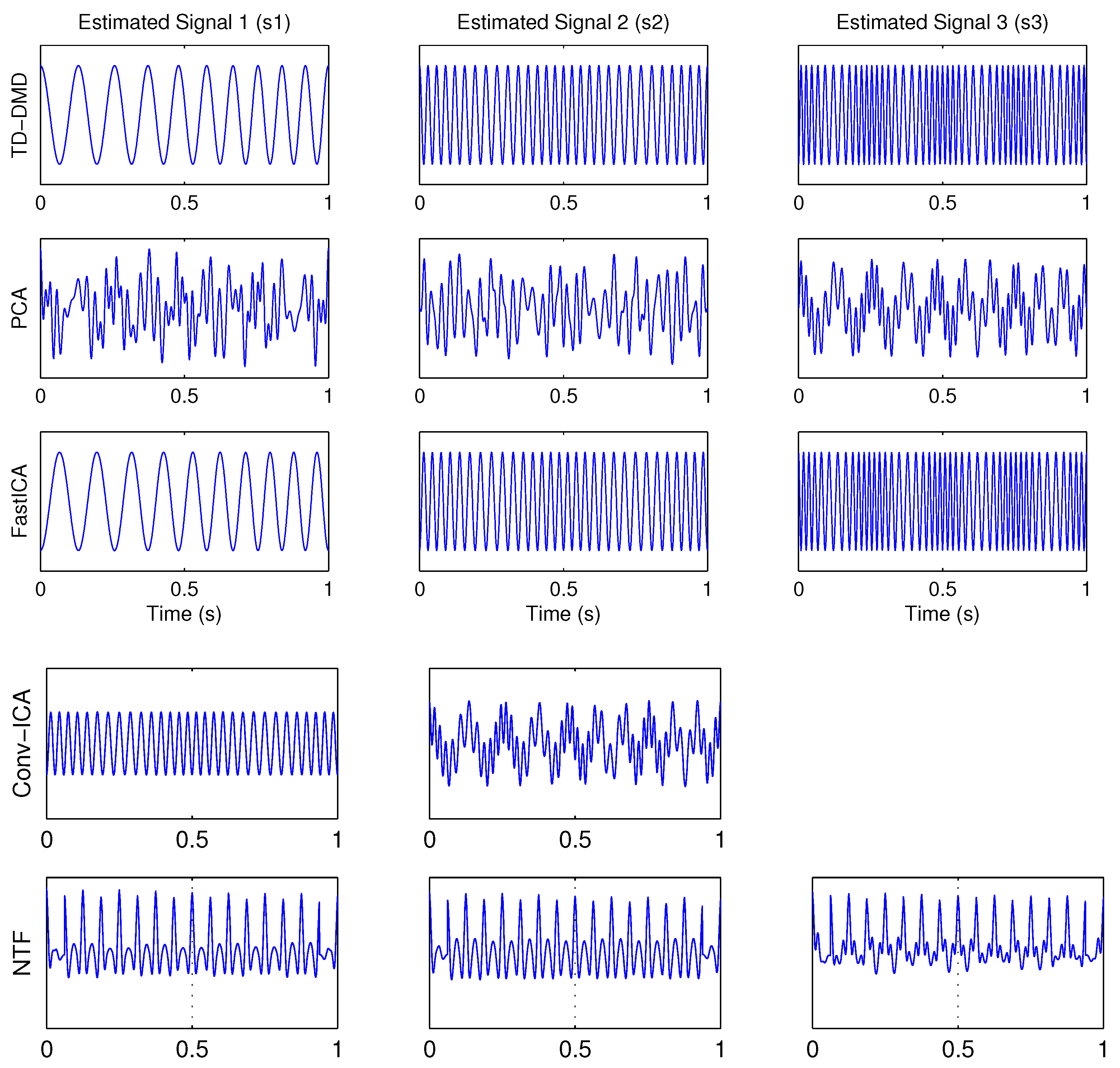
The resulting reconstruction of the latent signals, using TD-DMD with s = 2 , is identical to that obtained using the STIMD method in [39]. A comparison of estimated sources extracted from TD-DMD with s = 2 and the standard blind signal separation algorithms PCA, FastIca, Conv-ICA and NTF is shown in Figure 3.
The reconstructions obtained by PCA are obviously still a mixture of the measured signals. The results from NTF are also unsatisfactory. The Conv-ICA produces only two signals. Although the signals are statistically independent, their overlapping harmonics and phase modulations make it difficult for Conv-ICA to distinguish them in the frequency domain. The estimated signals by FastICA and TD-DMD, aside from a small amount of amplitude modulation that is not present in the true signals (they all have amplitude 1), are almost identical to the original signals.
The evaluation of the efficiency of separating mixed signals is computed using the correlation coefficient, which is calculated using the formula:
C o r r ( s i , s ^ j ) = t = 1 n s i ( t ) s ^ j ( t ) t = 1 n s i 2 ( t ) t = 1 n s ^ j 2 ( t ) ,
The results displayed in Figure 3 are also confirmed by the calculated similarity coefficients presented in Table 1.

4.2. Example 2: Separating Audio Signals

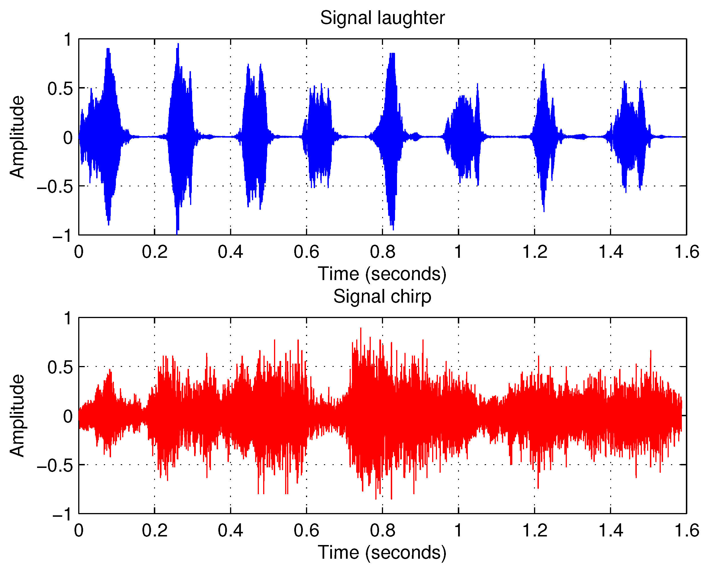
In this example, we will illustrate that TD-DMD approach can reconstruct mixed audio signals. We use two audio signals, which are built-in functions in Matlab. The first signal contains the sound of a bird chirping (‘chirp’), and the second contains a recording of a group of people laughing (‘laughter’). The two signals have n = 13,000 samples taken at 8.2 kHz, for a duration of 1.65 s each. We mix the signals with matrix
Q = 0.7 0.2 0.3 0.5 .
The two source signals are shown in Figure 4.
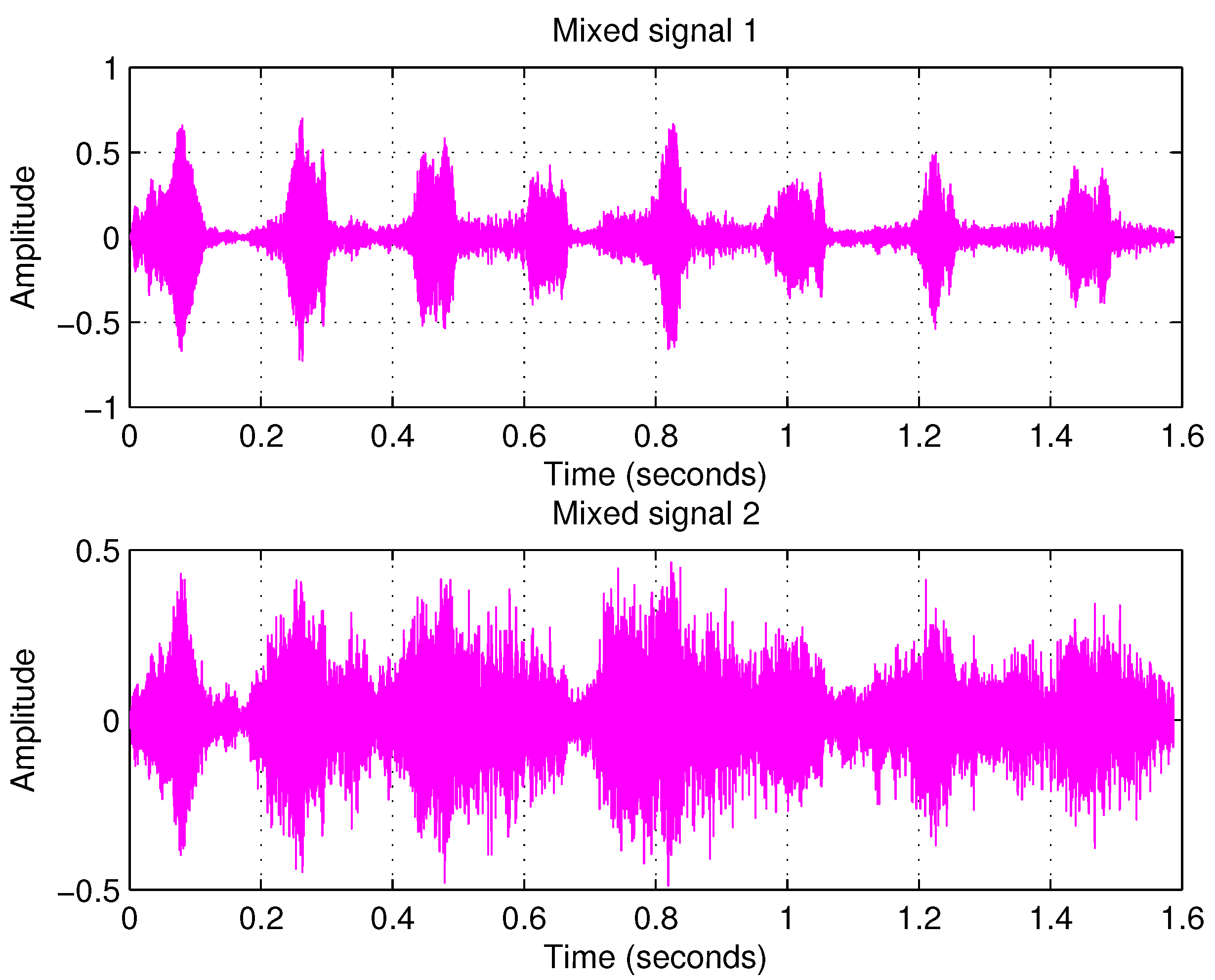
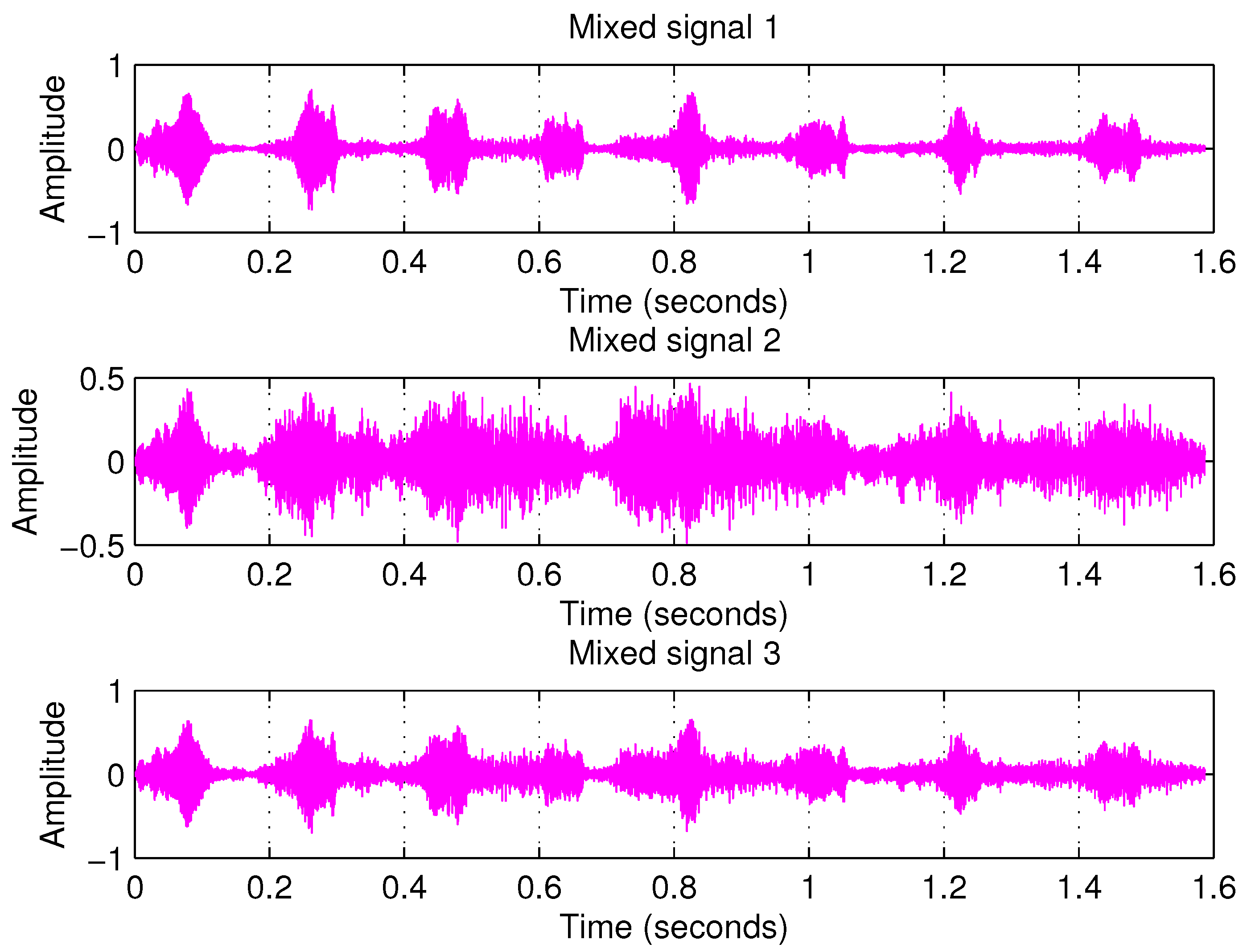
The observed signals are shown in Figure 5.
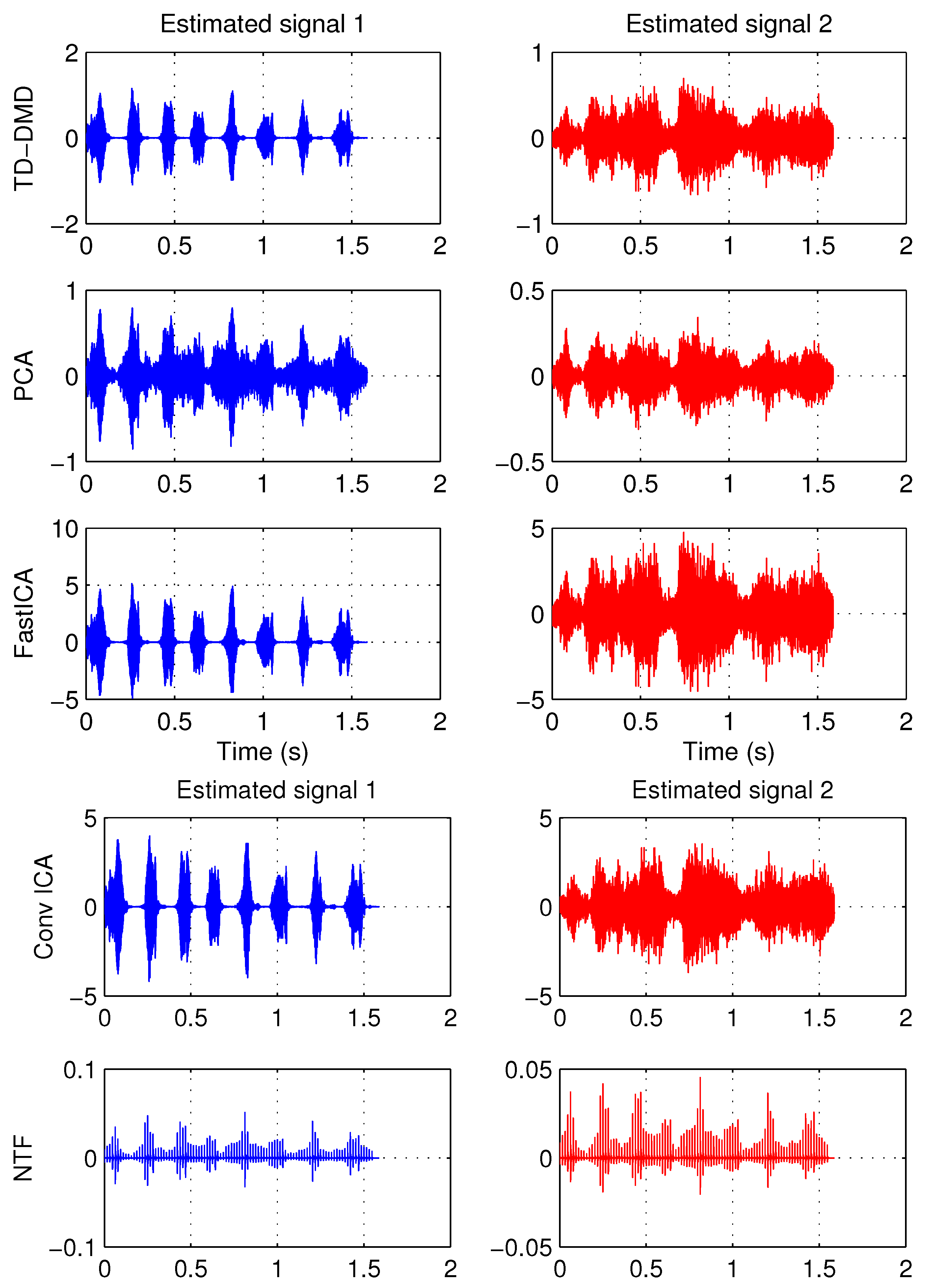
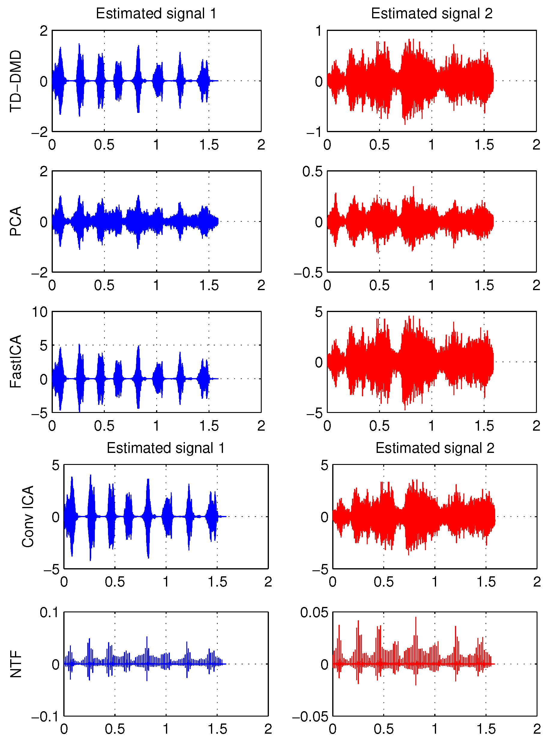
Figure 6 shows the estimates produced by the PCA, FastICA, Conv-ICA, NTF and TD-DMD, with  s = 2 . In this case, TD-DMD gives comparable results when choosing s = 1 and s = 2 .
Employing the PCA on observed signals does not work well here because the mixing matrix is not orthogonal. The most unsatisfactory results are obtained from the NTF method.
To assess the quality of the reconstructed signals, we used the popular metric Signal-to-noise ratio (SNR), which is calculated using the following formula:
S N R = 10 * log 10 i = 1 n s i 2 i = 1 n ( s i s ^ i ) 2 ,
where s i and s ^ i are the original and estimated sources, respectively.
The calculated similarity coefficients presented in Table 2 confirm the visualized results.

Overdetermined Case

To illustrate the application of Algorithm 1 in the overdetermined case, we will use the following mixing matrix:
Q = 0.7 0.2 0.3 0.5 0.6 0.4
The result is three observable signals, shown in Figure 7.
We note that in this case the standard (exact) DMD approach is not applicable. The proposed scheme (Algorithm 1) effectively separates the two signals. Separated signals by TD-DMD, with  s = 2 , PCA, FastICA, Conv-ICA and NTF are shown in Figure 8.
In this case, although the reproduced results are similar, s = 1 yields slightly better results than s = 2 . The PCA and NTF methods do not produce satisfactory results. This is also seen in Table 3.

4.3. Example 3: Separation of Mixed Images

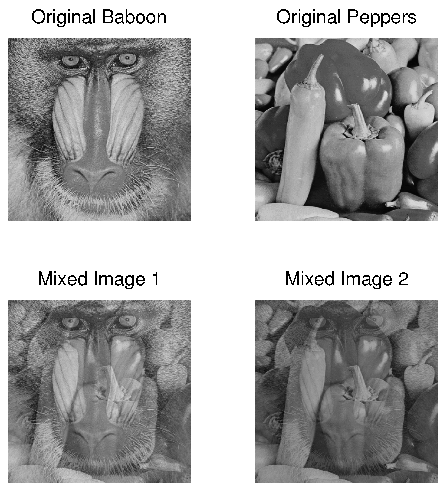
In this example, we will use a mixture of two standard images Baboon and Pepper. Both images are grayscale images with 256 × 256 pixels. The two mixed images, see Figure 9, are obtained by the mixing matrix
Q = 0.6 0.4 0.3 0.5
The original images and linear mixed images ar shown in Figure 9.
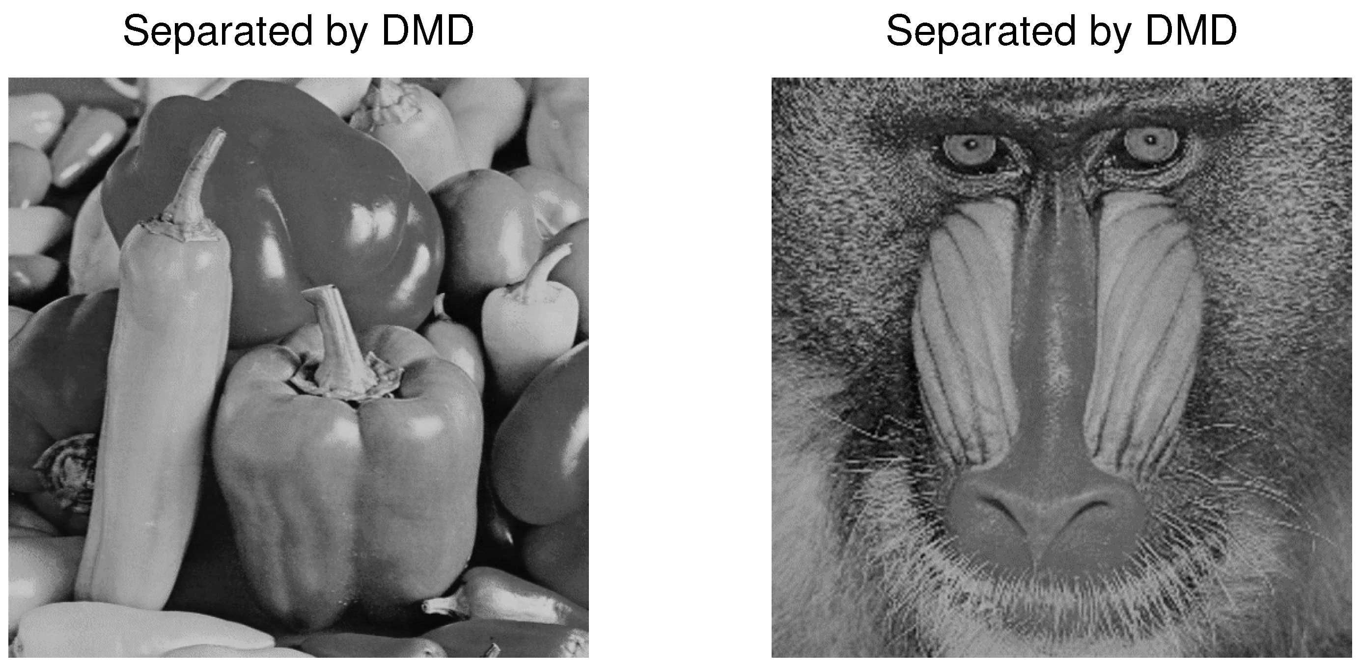
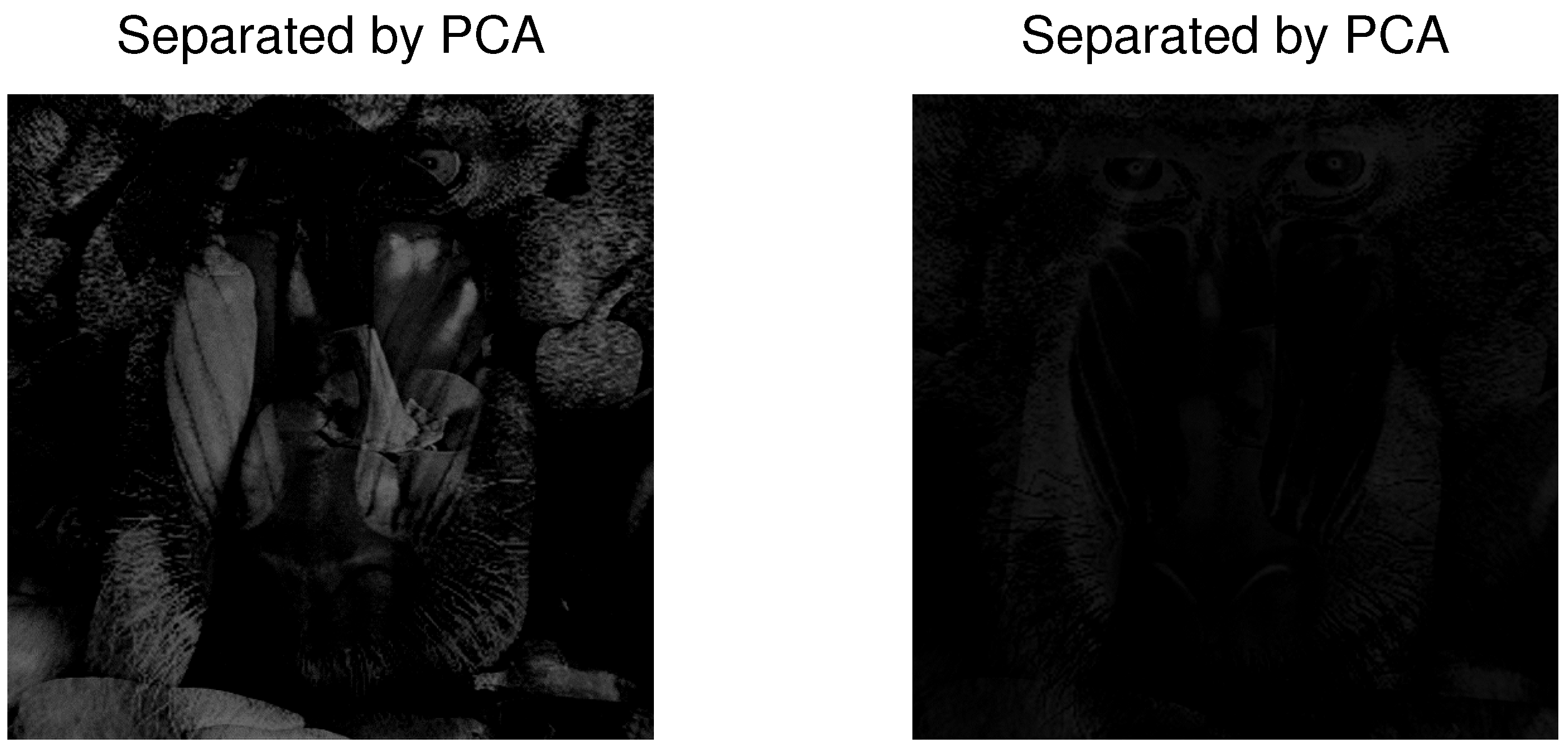
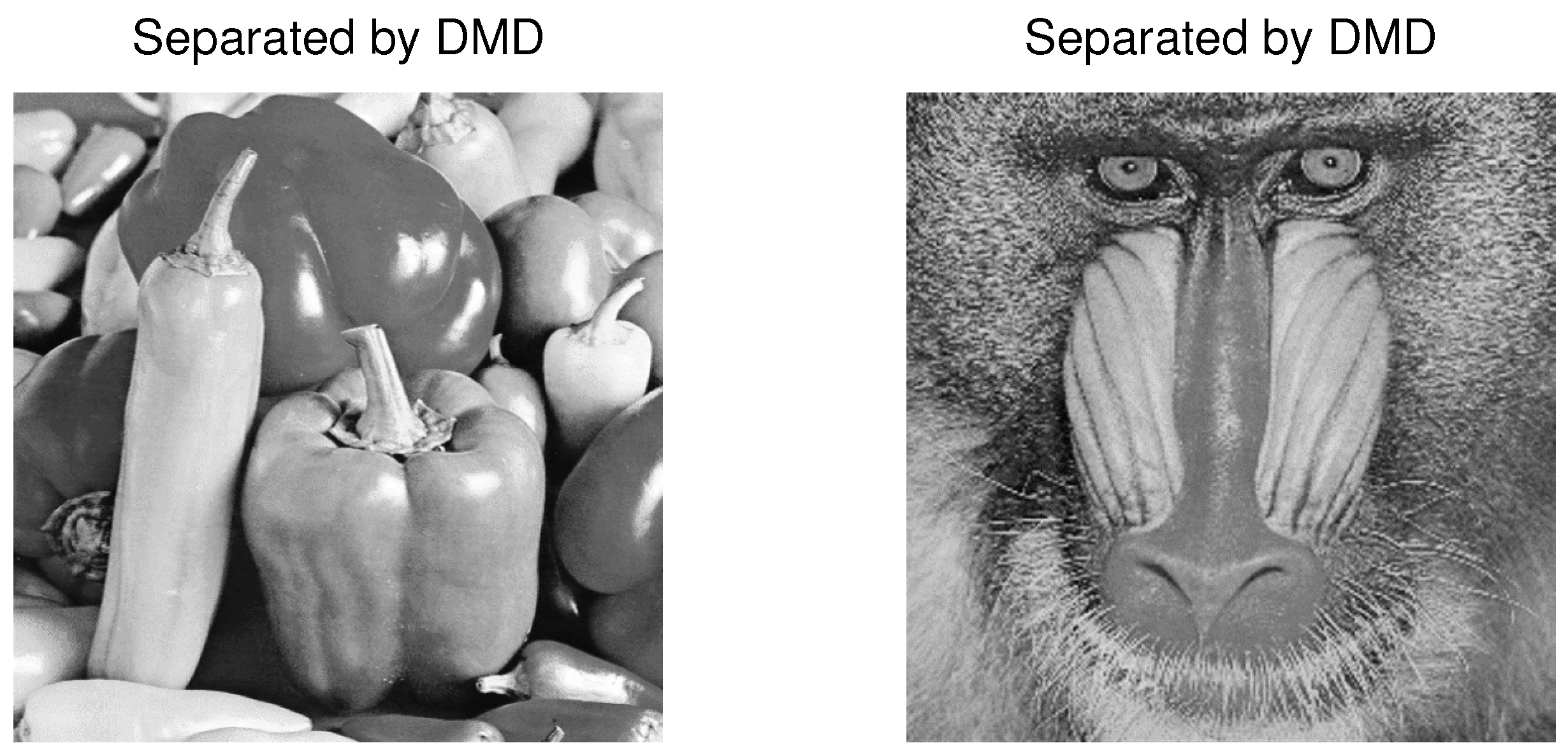
The separated source images by TD-DMD and PCA are shown in Figure 10 and Figure 11, respectively.
NTF fails to separate two mixed images, because it assumes that both the source signals and the mixing coefficients are nonnegative, but the mixing matrix Q does not preserve strict nonnegativity for all pixel combinations. The ICA and Conv-ICA methods also fail because the mixing matrix Q is nearly ill-conditioned, making separation difficult. The visualization of the results from the application of the NTF, ICA and Conv-ICA methods is omitted, as they are worse than the result of the PCA method, shown in Figure 11.
Table 4 shows: the estimated mixing matrix Φ , the matrix product Φ 1 Q and Mean Square Error of the approximation of Q by Φ , for different values of s.
The calculated similarity coefficients presented in Table 5 confirm the visualized results.

Overdetermined Case

We show TD-DMD applied to the case of three observed signals and two source signals. The mixed images obtained by the overdetermined mixing matrix:
Q = 0.6 0.4 0.3 0.5 0.5 0.5
Mixed images are shown in Figure 12.
The best results from Algorithm 1 are achieved at s = 2 . The resulting estimate of the mixing matrix is
Φ = 0.5684 0.3571 0.2767 0.4362 0.4695 0.4407 ,
and the matrix product Φ 1 Q is the following:
Φ 1 Q = 1.1636 0.0302 0.0274 1.0367 .
Separated images by TD-DMD, with  s = 2 , are shown in Figure 13.
The calculated similarity coefficients presented in Table 6 confirm the visualized results.

4.4. Example 4: Analysis of EEG-Data

An electroencephalogram (EEG) is a test to assess electrical activity in the brain that uses small electrodes attached to the scalp. It is known that the main means of communication between brain cells, which are always active, even when you are sleeping, are electrical impulses [57,58]. EEG studies find application in the therapeutic environment for the diagnosis and treatment of neurological diseases, including multiple sclerosis, epilepsy, and other mental illnesses [59]. But the EEG signal is often contaminated by the so called artifacts [60]. These are unwanted signals from sources other than the brain that alter the original EEG activity and complicate its interpretation [61]. Artifacts are divided into physiological and non-physiological. Physiological artifacts are: biological activity of the eye, muscles, heart, breathing, etc. While interference from instruments and moving electrodes, wires, electromagnetic fields, etc. are classified as non-physiological artifacts [62]. The main problem when working with EEG data is still the reduction of artifacts. Various approaches are known to address this problem, one of the methods used to remove artifacts is Blind Sources Separation (BSS) [63].
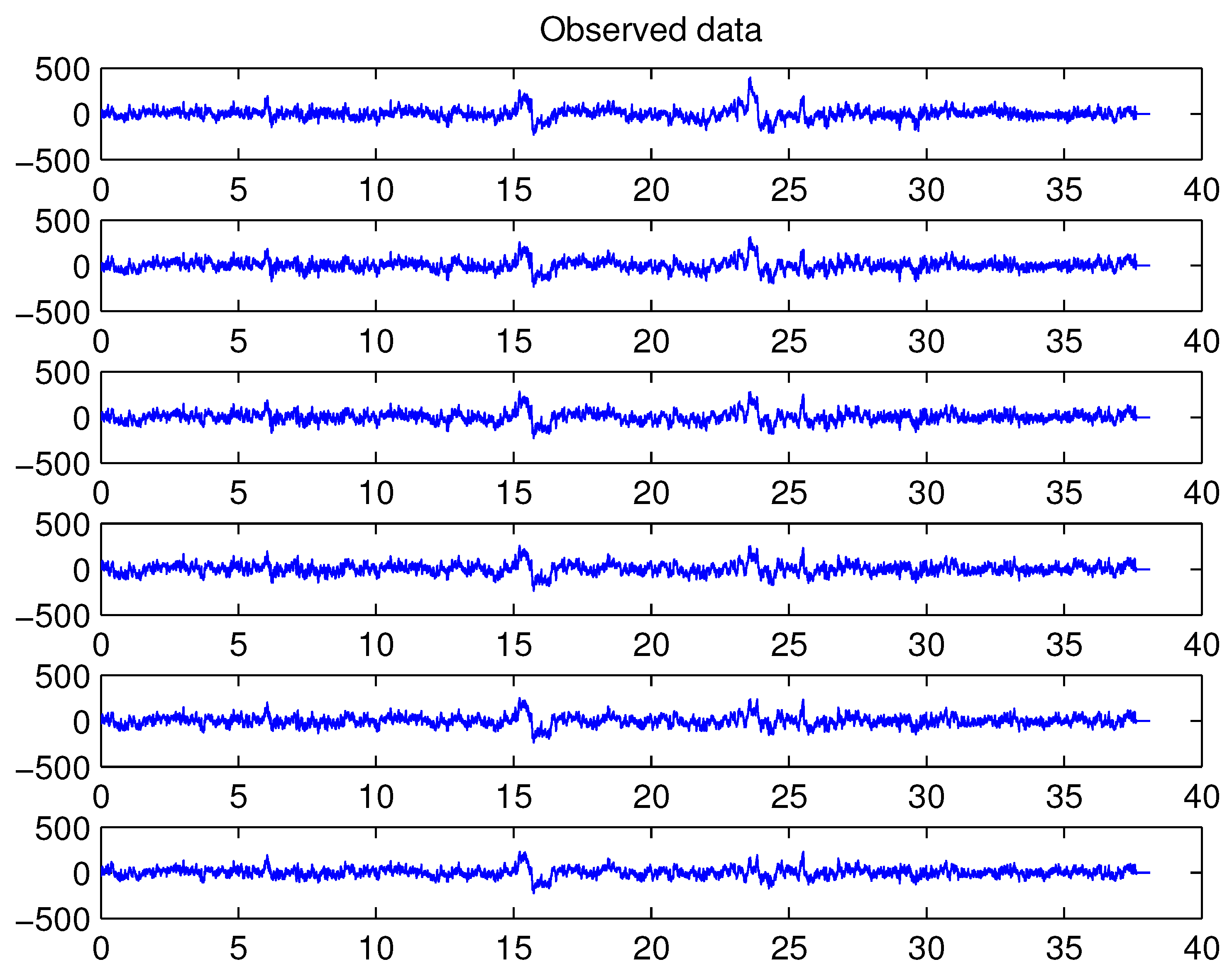
In this example we use real EEG data from PhysioNet database [64]. This data set consists of over 1500 one- and two-minute EEG recordings, obtained from 109 volunteers. Subjects performed different motor/imagery tasks while 64-channel EEG were recorded using the BCI2000 system (http://www.bci2000.org, , accessed on 18 December 2024). The EEGs are recorded from 64 electrodes as per the international 10-10 system. The data are provided in EDF+ format (containing 64 EEG signals, each sampled at 160 samples per second). The file “S001R01.edf” was used for the experiments here. Figure 14 visualizes the first six signals of the recorded data.
Before applying the DMD approach, we prepare the data by filtering and centering it. After preprocessing the data, we applied Algorithm 1 with different values of the time-delay coefficient s. Sometimes it is possible to visually verify which components correspond to different artifacts.
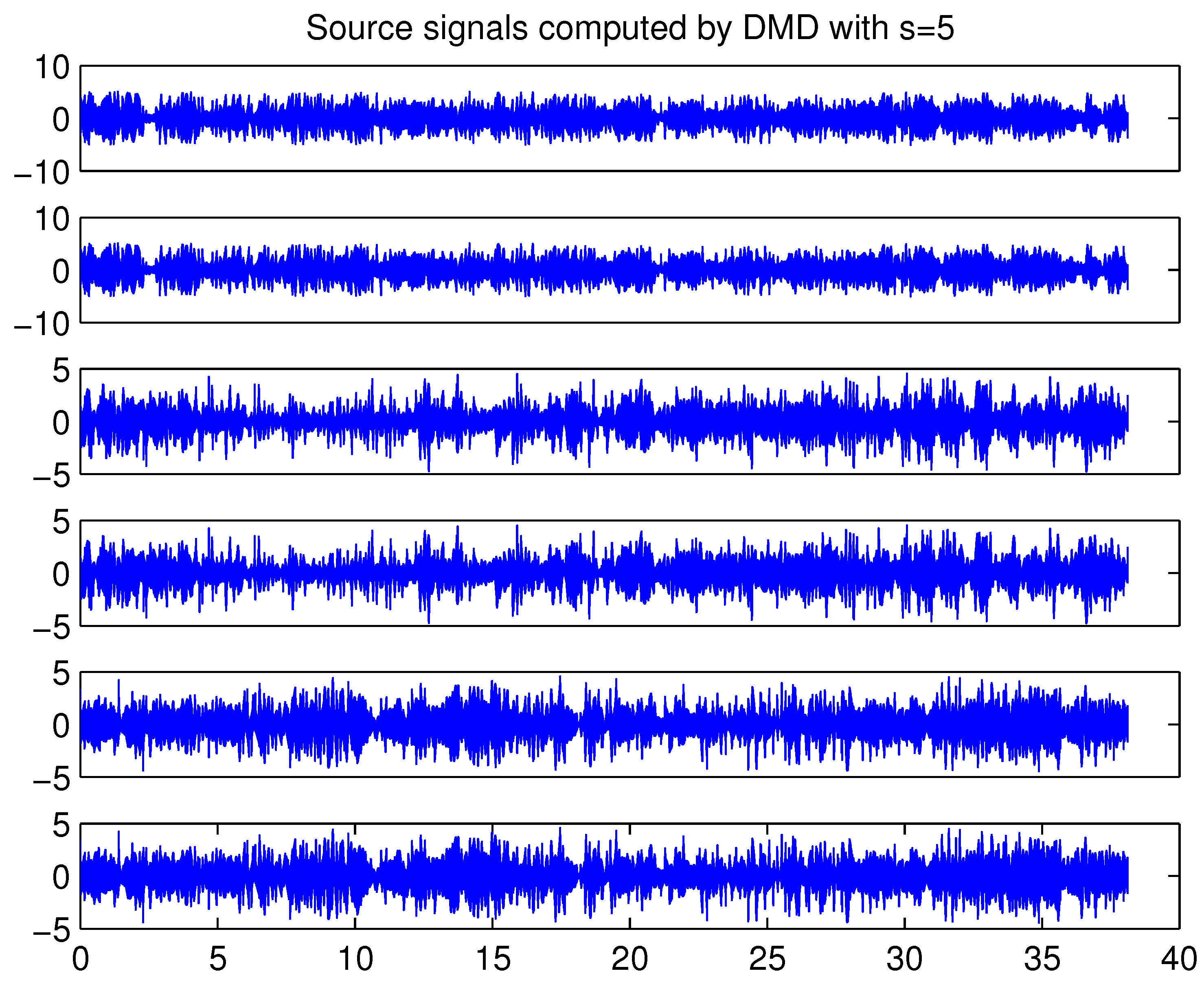
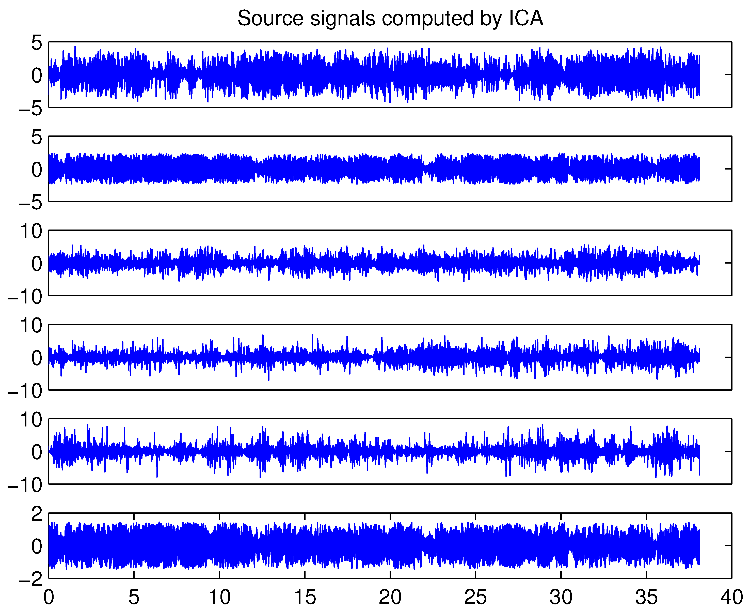
Figure 15 shows a visualization of the source signals at s = 5 . It is already clear from the graph that the sources are three signals that are repeated, i.e., we have three pairs of correlating signals. This dependence is preserved for different values of s > 1 , as the correlation between repeated signals increases with increasing s. This leads us to the conclusion that there are three independent source signals.
To compare the obtained results with those from the ICA method, we use the runica function from the EEGLAB tools of Matlab. The same preprocessing of the initial data that was applied in Algorithm 1 is used here. Figure 16 visualizes the separated signals using the ICA method. Examining the correlation between the three signals obtained through Algorithm 1 and the signals obtained from the ICA, it is found that there is a high correlation between them. Moreover, this correlation is greater for larger values of s.
For example, at s = 5 we have the following correlation indices:
C o r r ( s 1 , s ¯ 1 ) = 0.5731 , C o r r ( s 3 , s ¯ 4 ) = 0.6449 and C o r r ( s 5 , s ¯ 3 ) = 0.6816
and at s = 20 , we get
C o r r ( s 1 , s ¯ 3 ) = 0.7682 , C o r r ( s 3 , s ¯ 2 ) = 0.8591 and C o r r ( s 5 , s ¯ 6 ) = 0.7222 ,
where s i denotes the signals computed by TD-DMD and s ¯ i denotes the signals computed by ICA.

5. Conclusions

The aim of this study was to introduce an extended approach of the DMD method to implement the BSS task. While DMD is successful for many tasks, its standard form is limited by its lack of ability to capture complex time dependencies, which are key for BSS. The presented modification uses the SVD-based DMD scheme by using delay embedding techniques. Introducing time delays into DMD extends its scope and allows the method to extract more information about the dynamics of the system. The matrix representations underlying this technique are provided, highlighting their corresponding computational frameworks for solving the BSS model. The proposed algorithm extends the possibilities of the DMD approach to be used in the case of an overdetermined BSS model. Furthermore, the scheme is applicable to various, predefined, time lag. In particular, the algorithm can be reduced to a standard (exact) DMD approach with a single time lag. We have demonstrated the performance of the presented algorithm with various illustrative numerical examples, including separation of audio signals and images. An experimental comparison with traditional techniques such as ICA and PCA is presented. Numerical results show that the introduced algorithm outperforms the standard DMD approach in most cases. It is also illustrated that it is applicable in some cases where standard approaches such as PCA or ICA do not yield good results. The numerical results show that the introduced algorithm is an alternative for solving the BSS and can be used in various fields of application.
Some potential avenues for future development in this line of research are:
  • Extension to Nonlinear Dynamics: While our current approach primarily addresses linear dynamics, we aim to investigate the extension of DMD-based BSS to handle nonlinear systems through methods such as kernel DMD or deep learning-enhanced DMD.
  • Real-Time and Online Implementations: Another direction is to develop real-time or online implementations of DMD-based BSS for applications in robotics, communications, and biomedical signal processing, where real-time performance is critical.
  • Parallel Implementation: One of the key areas for future research will involve implementing the DMD-based BSS method in a parallel computing environment. This would allow us to efficiently process larger datasets and reduce computational times, making the method more suitable for real-time applications.
  • Integration with Deep Learning Techniques: Combining DMD approach with machine learning and deep learning methods is another promising area of research. This could involve using neural networks to improve the performance and robustness of the DMD-based BSS in complex or noisy environments.
This work highlights TD-DMD as a powerful tool for combining dynamical systems analysis and signal processing, paving the way for further advancements in BSS and dynamic data decomposition.

Funding

This research received no external funding.

Data Availability Statement

No additional data.

Conflicts of Interest

The authors declare no conflicts of interest.

References

  1. Hérault, J.; Ans, B. Circuits neuronaux à synapses modifiables: Décodage de messages composites par apprentissage non supervisé. Comptes Rendus Acad. Sci. 1984, 299, 525–528. [Google Scholar]
  2. Hérault, J.; Jutten, C. Space or time adaptive signal processing by neural networks models. In Proceedings of the International Conference on Neural Networks for Computing, Snowbird, UT, USA, 13–16 April 1986; pp. 206–211. [Google Scholar]
  3. Comon, P.; Jutten, C.; Hérault, J. Blind separation of sources, Part II: Problem statement. Signal Process. 1991, 24, 11–20. [Google Scholar] [CrossRef]
  4. Sorouchyari, E. Blind separation of sources, Part III: Stability analysis. Signal Process. 1991, 24, 21–29. [Google Scholar] [CrossRef]
  5. Makino, S.; Lee, T.-W.; Sawada, H. Blind Speech Separation. In Signals and Communication Technology; Springer: Berlin/Heidelberg, Germany, 2007. [Google Scholar]
  6. Falk, R.H. Medical progress: Atrial fibrillation. N. Engl. J. Med. 2001, 344, 1067–1078. [Google Scholar] [CrossRef] [PubMed]
  7. Rieta, J.J.; Castells, F.; Snchez, C.; Zarzoso, V.; Millet, J. Atrial activity extraction for atrial fibrillation analysis using blind source separation. IEEE Trans. Biomed. Eng. 2004, 51, 1176–1186. [Google Scholar] [CrossRef]
  8. Hyvärinen, A.; Karhunen, J.; Oja, E. Independent Component Analysis; Wiley: Hoboken, NJ, USA, 2001. [Google Scholar]
  9. Yu, H.; Deng, X.; Tang, J.; Yue, F. Patterns Identification Using Blind Source Separation with Application to Neural Activities Associated with Anticipated Falls. Inf. Sci. 2025, 689, 121410. [Google Scholar] [CrossRef]
  10. Wang, Q.; Zhang, L.; Bertinetto, L.; Hu, W.; Torr, P.H. Fast online object tracking and segmentation: A unifying approach. In Proceedings of the IEEE/CVF Conference on Computer Vision and Pattern Recognition, Long Beach, CA, USA, 15–20 June 2019; pp. 1328–1338. [Google Scholar]
  11. Wang, X.; Huang, D.-S. A novel multi-layer level set method for image segmentation. J. Univers. Comput. Sci. 2008, 14, 2427–2452. [Google Scholar]
  12. Zhao, Y.; Huang, D.-S.; Jia, W. Completed local binary count for rotation invariant texture classification. IEEE Trans. Image Process. 2012, 21, 4492–4497. [Google Scholar] [CrossRef]
  13. Wang, X.-F.; Huang, D.-S.; Du, J.-X.; Xu, H.; Heutte, L. Classification of plant leaf images with complicated background. Appl. Math. Comput. 2008, 205, 916–926. [Google Scholar] [CrossRef]
  14. Man, L.; Zhu, C. Research on Signal Separation Method for Moving Group Target Based on Blind Source Separation. In Proceedings of the ICCIP ’23: 2023 9th International Conference on Communication and Information Processing, Lingshui, China, 14–16 December 2023; pp. 256–260. [Google Scholar]
  15. Chang, S.; Deng, Y.; Zhang, Y.; Zhao, Q.; Wang, R.; Zhang, K. An Advanced Scheme for Range Ambiguity Suppression of Spaceborne SAR Based on Blind Source Separation. IEEE Trans. Geosci. Remote. Sens. 2022, 60, 5230112. [Google Scholar] [CrossRef]
  16. Badaracco, F.; Banerjee, B.; Branchesi, M.; Chincarini, A. Blind source separation in 3rd generation gravitational-wave detectors. New Astron. Rev. 2024, 99, 101707. [Google Scholar] [CrossRef]
  17. Tolmachev, D.; Chertovskih, R.; Jeyabalan, S.R.; Zheligovsky, V. Predictability of Magnetic Field Reversals. Mathematics 2024, 12, 490. [Google Scholar] [CrossRef]
  18. Lee, T.-W. Independent component analysis. In Independent Component Analysis: Theory and Applications; Springer: New York, NY, USA, 1998; pp. 27–66. [Google Scholar]
  19. Hyvärinen, A.; Oja, E. Independent component analysis: Algorithms and applications. Neural Netw. 2000, 13, 411–430. [Google Scholar] [CrossRef]
  20. Jolliffe, I.T. Principal Component Analysis; Springer: New York, NY, USA; Berlin/Heidelberg, Germany, 1986. [Google Scholar]
  21. Lee, D.; Seung, H.S. Algorithms for non-negative matrix factorization. In Advances in Neural Information Processing Systems; Leen, T.K., Dietterich, T.G., Tresp, V., Eds.; MIT Press: Cambridge, MA, USA, 2000; pp. 535–541. [Google Scholar]
  22. Hyvärinen, A.; Hoyer, P.O. Emergence of phase-and shift-invariant features by decomposition of natural images into independent feature subspaces. Neural Comput. 2000, 12, 1705–1720. [Google Scholar] [CrossRef]
  23. Prasadan, A.; Nadakuditi, R. The finite sample performance of Dynamic Mode Decomposition. In Proceedings of the 2018 IEEE Global Conference on Signal and Information Processing (GlobalSIP), Anaheim, CA, USA, 26–29 November 2018; IEEE: Piscataway, NJ, USA, 2018; pp. 1–5. [Google Scholar]
  24. Creager, E.; Stein, N.D.; Badeau, R.; Depalle, P. Nonnegative tensor factorization with frequency modulation cues for blind audio source separation. arXiv 2016, arXiv:1606.00037. [Google Scholar]
  25. Belouchrani, A.; Meraim, K.A.; Cardoso, J.F. A blind source separation technique based on second order statistics. IEEE Trans. Signal Process. 2002, 45, 434–444. [Google Scholar] [CrossRef]
  26. Webster, M.B.; Lee, J. Blind Source Separation of Single-Channel Mixtures via Multi-Encoder Autoencoders. arXiv 2024, arXiv:2309.07138. [Google Scholar]
  27. Erdogan, A.T.; Pehlevan, C. Blind Bounded Source Separation Using Neural Networks with Local Learning Rules. In Proceedings of the ICASSP 2020-2020 IEEE International Conference on Acoustics, Speech and Signal Processing (ICASSP), Barcelona, Spain, 4–8 May 2020; IEEE: Piscataway, NJ, USA, 2020; pp. 3812–3816. [Google Scholar]
  28. Bando, Y.; Masuyama, Y.; Nugraha, A.A.; Yoshii, K. Neural Fast Full-Rank Spatial Covariance Analysis for Blind Source Separation. arXiv 2023, arXiv:2306.10240. [Google Scholar]
  29. Yu, X.; Hu, D.; Xu, J. Blind Source Separation—Theory and Applications; John Wiley and Sons: New York, NY, USA, 2014. [Google Scholar]
  30. Hassan, N.; Ramli, D.A. A comparative study of blind source separation for bioacoustics sounds based on FastICA, PCA and NMF. Procedia Comput. Sci. 2018, 126, 363–372. [Google Scholar] [CrossRef]
  31. Tharwat, A. Independent component analysis: An introduction. Appl. Comput. Inform. 2021, 17, 222–249. [Google Scholar] [CrossRef]
  32. Baysal, B.; Efe, M. A comparative study of blind source separation methods. Turk. J. Electr. Eng. Comput. Sci. 2023, 31, 9. [Google Scholar] [CrossRef]
  33. Schmid, P.J.; Sesterhenn, J. Dynamic mode decomposition of numerical and experimental data. In Proceedings of the 61st Annual Meeting of the APS Division of Fluid Dynamics, San Antonio, TX, USA, 23–25 November 2008; American Physical Society: College Park, MD, USA, 2008. [Google Scholar]
  34. Prasadan, A.; Lodhia, A.; Nadakuditi, R.R. Phase transitions in the dynamic mode decomposition algorithm. In Proceedings of the Computational Advances in Multi-Sensor Adaptive Processing, Le Gosier, Guadeloupe, 15–18 December 2019; IEEE: Piscataway, NJ, USA, 2019; pp. 1–5. [Google Scholar]
  35. Prasadan, A.; Nadakuditi, R. Time Series Source Separation Using Dynamic Mode Decomposition. Siam J. Appl. Dyn. 2020, 19, 1160–1199. [Google Scholar] [CrossRef]
  36. Chen, C.; Peng, H. Dynamic mode decomposition for blindly separating mixed signals and decrypting encrypted images. Big Data And Inf. Anal. 2024, 8, 1–25. [Google Scholar] [CrossRef]
  37. Nedzhibov, G.H. On Alternative Algorithms for Computing Dynamic Mode Decomposition. Computation 2022, 10, 210. [Google Scholar] [CrossRef]
  38. Tu, J.H.; Rowley, C.W.; Luchtenburg, D.M.; Brunton, S.L.; Kutz, J.N. On dynamic mode decomposition: Theory and applications. J. Comput. Dyn. 2014, 1, 391–421. [Google Scholar] [CrossRef]
  39. Hirsh, S.M.; Brunton, B.W.; Kutz, J.N. Data-driven Spatiotemporal Modal Decomposition for Time Frequency Analysis. Appl. Comput. Harmon. Anal. 2020, 49, 771–790. [Google Scholar] [CrossRef]
  40. Takens, F. Detecting Strange Attractors in Turbulence, in Dynamical Systems and Turbulence; Lecture Notes in Math; Springer: Berlin/Heidelberg, Germany, 1981; Volume 898. [Google Scholar]
  41. Clainche, S.L.; Vega, J.M. Higher order dynamic mode decomposition. SIAM J. Appl. Dyn. Syst. 2017, 16, 882–925. [Google Scholar] [CrossRef]
  42. Vega, J.M.; Clainche, S.L. Higher Order Dynamic Mode Decomposition and Its Applications; Academic Press: London, UK, 2021; ISBN 9780128227664. [Google Scholar]
  43. Nedzhibov, G.H. On Higher Order Dynamic Mode Decomposition. Ann. Acad. Rom. Sci. Ser. Math. Appl. 2024, 16, 5–16. [Google Scholar] [CrossRef]
  44. Williams, M.O.; Hemati, M.S.; Dawson, S.T.M.; Kevrekidis, I.G.; Rowley, C.W. Extending Data-Driven Koopman Analysis to Actuated Systems. IFAC-PapersOnLine 2016, 49, 704–709. [Google Scholar] [CrossRef]
  45. Anantharamu, S.; Mahesh, K. A parallel and streaming Dynamic Mode Decomposition algorithm with finite precision error analysis for large data. J. Comput. Phys. 2019, 380, 355–377. [Google Scholar] [CrossRef]
  46. Li, B.; Garicano-Menaab, J.; Valero, E. A dynamic mode decomposition technique for the analysis of nonuniformly sampled flow data. J. Comput. Phys. 2022, 468, 111495. [Google Scholar] [CrossRef]
  47. Mezić, I. On Numerical Approximations of the Koopman Operator. Mathematics 2022, 10, 1180. [Google Scholar] [CrossRef]
  48. Nedzhibov, G. Dynamic Mode Decomposition: A new approach for computing the DMD modes and eigenvalues. Ann. Acad. Rom. Sci. Ser. Math. Appl. 2022, 14, 5–16. [Google Scholar] [CrossRef]
  49. Nedzhibov, G. An Improved Approach for Implementing Dynamic Mode Decomposition with Control. Computation 2023, 11, 201. [Google Scholar] [CrossRef]
  50. Nedzhibov, G. Online Dynamic Mode Decomposition: An alternative approach for low rank datasets. Ann. Acad. Rom. Sci. Ser. Math. Appl. 2023, 15, 229–249. [Google Scholar] [CrossRef]
  51. Nedzhibov, G. Delay-Embedding Spatio-Temporal Dynamic Mode Decomposition. Mathematics 2024, 12, 762. [Google Scholar] [CrossRef]
  52. Arbabi, H.; Mezic, I. Ergodic Theory, Dynamic Mode Decomposition, and Computation of Spectral Properties of the Koopman Operator. SIAM J. Appl. Dyn. Syst. 2017, 16, 2096–2126. [Google Scholar] [CrossRef]
  53. Kamb, M.; Kaiser, E.; Brunton, S.L.; Kutz, J.N. Time-delay observables for Koopman: Theory and applications. SIAM J. Appl. Dyn. Syst. 2020, 19, 886–917. [Google Scholar] [CrossRef]
  54. Kutz, J.N.; Brunton, S.L.; Brunton, B.W.; Proctor, J. Dynamic Mode Decomposition: Data-Driven Modeling of Complex Systems; SIAM: Philadelphia, PA, USA, 2016; ISBN 978-1-611-97449-2. [Google Scholar]
  55. Wu, Z.; Brunton, S.L.; Revzen, S. Challenges in dynamic mode decomposition. arXiv 2021, arXiv:2109.01710. [Google Scholar] [CrossRef] [PubMed]
  56. Yuan, Y.; Zhou, K.; Zhou, W.; Wen, X.; Liu, Y. Flow prediction using dynamic mode decomposition with time-delay embedding based on local measurement. Phys. Fluids 2021, 33, 095109. [Google Scholar] [CrossRef]
  57. Massar, H.; Nsiri, B.; Drissi, T.B. DWT-BSS: Blind Source Separation applied to EEG signals by extracting wavelet transform’s approximation coefficients. J. Phys. Conf. Ser. 2023, 2550, 012031. [Google Scholar] [CrossRef]
  58. EEG (Electroencephalogram). Mayo Clinic. Mayo Foundation for Medical Education and Research. 2022. Available online: https://www.mayoclinic.org/tests-procedures/eeg/about/pac-20393875 (accessed on 17 November 2022).
  59. Judith, A.M.; Priya, S.B.; Mahendran, R.K. Artifact Removal from EEG signals using Regenerative Multi-Dimensional Singular Value Decomposition and Independent Component Analysis. Biomed. Signal Process. Control. 2022, 74, 103452. [Google Scholar]
  60. Kachenoura, A.; Albera, L.; Senhadji, L. Séparation aveugle de sources en ingénierie biomédicale. IRBM 2007, 28, 20–34. [Google Scholar] [CrossRef]
  61. Mannan, M.M.N.; Kamran, M.A.; Jeong, M.Y. Identification and removal of physiological artifacts from electroencephalogram signals: A review. IEEE Access 2018, 6, 30630–30652. [Google Scholar] [CrossRef]
  62. Rashmi, C.R.; Shantala, C.P. EEG artifacts detection and removal techniques for braincomputer interface applications: A systematic review. Int. J. Adv. Technol. Eng. Explor. 2022, 9, 354. [Google Scholar]
  63. Zhou, W.; Chelidze, D. Blind source separation based vibration mode identification. Mech. Syst. Signal Process. 2007, 21, 3072–3087. [Google Scholar] [CrossRef]
  64. Schalk, G.; McFarland, D.J.; Hinterberger, T.; Birbaumer, N.; Wolpaw, J.R. BCI2000: A General-Purpose Brain-Computer Interface (BCI) System. IEEE Trans. Biomed. Eng. 2004, 51, 1034–1043. [Google Scholar] [CrossRef] [PubMed]
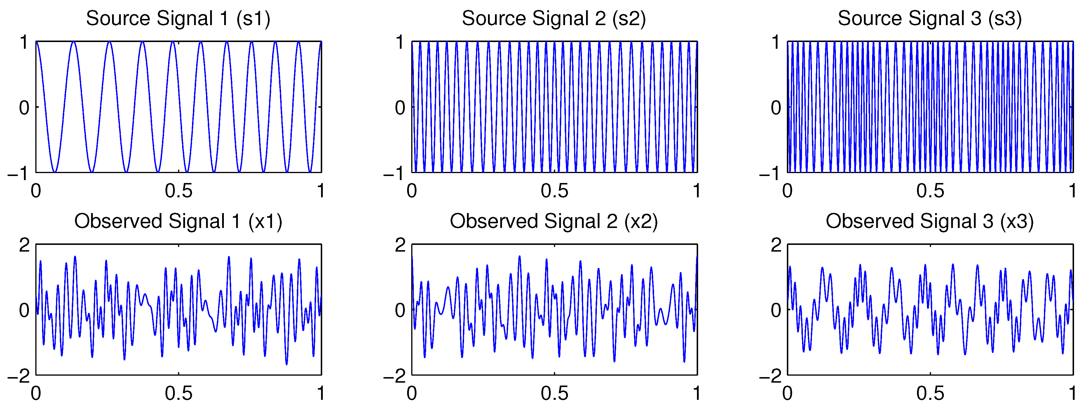
Figure 1. Three-dimensional system defined by (37). Row 1: The three true source signals. Row 2: The observed mixed measurement signals.
Computation 13 00031 g001
Figure 2. Estimated source signals by Time-Delay DMD, with s = 1 , in blue. The tree true source signals in red dotted lines.
Computation 13 00031 g002
Figure 3. Comparison of estimated sources extracted by: Row 1: Time-Delay DMD, with s = 2 ; Row 2: PCA method; Row 3: FastICA method; Row 4: Conv-ICA method; Row 5: NTF method.
Computation 13 00031 g003
Figure 4. The two original audio signals.
Computation 13 00031 g004
Figure 5. The linear mixed images.
Computation 13 00031 g005
Figure 6. Separated signals by TD-DMD (with s = 2 ), PCA, FastICA, Conv-ICA and NTF.
Computation 13 00031 g006
Figure 7. Three mixed images.
Computation 13 00031 g007
Figure 8. Separated signals by TD-DMD (with s = 2 ), PCA, FastICA, Conv-ICA and NTF.
Computation 13 00031 g008
Figure 9. Row 1: The original images. Row 2: The linear mixed images.
Computation 13 00031 g009
Figure 10. Separated images by TD-DMD, with s = 2 .
Computation 13 00031 g010
Figure 11. Separated images by PCA.
Computation 13 00031 g011
Figure 12. Mixed images in overdetermined case.
Computation 13 00031 g012
Figure 13. Separated images by TD-DMD with s = 2 .
Computation 13 00031 g013
Figure 14. First 6 signals of observed EEG data.
Computation 13 00031 g014
Figure 15. Source signals computed by TD-DMD, with s = 5 .
Computation 13 00031 g015
Figure 16. Source signals computed by Conv-ICA method.
Computation 13 00031 g016
Table 1. Correlation coefficients for PCA, FastICA, TD-DMD (with s = 2 ), Conv-ICA and NTF.
PCAFastICATD-DMDConv-ICANTF
C o r r ( s 1 , s ^ 1 ) 0.580450.998931-0.02403
C o r r ( s 2 , s ^ 2 ) −0.81851−0.99914−10.70950.4763
C o r r ( s 3 , s ^ 3 ) −0.70819−0.99975−10.9994−0.0052
Table 2. Signal to noise ratio (SNR) for PCA, FastICA, Conv-ICA, NTF and TD-DMD with s = 1 and s = 2 .
PCAFastICATD-DMD
( s = 1 )
TD-DMD
( s = 2 )
Conv-ICANTF
S N R ( s 1 , s ^ 1 ) 5.85−12.3712.42−6.66−10.09−0.002
S N R ( s 2 , s ^ 2 ) 0.51−14.68−3.7313.0412.420.33
Table 3. Signal to noise ratio (SNR), in the overdetermined case, for PCA, FastICA, Conv-ICA, NTF and TD-DMD with s = 1 and s = 2 .
PCAFastICATD-DMD
( s = 1 )
TD-DMD
( s = 2 )
Conv-ICANTF
S N R ( s 1 , s ^ 1 ) 4.59−15.7829.92−7.85−10.04−0.002
S N R ( s 2 , s ^ 2 ) −0.52−14.669.58−5.8812.420.3
Table 4. Estimated mixing matrix Φ , the product Φ 1 Q and MSE error for TD-DMD with s = 1 , 2 , 3 .
TD-DMD with Φ Φ 1 Q MSE
s = 1 0.9021 0.6331 0.4316 0.7740 0.6551 0.0275 0.0164 0.6458 0.0595
s = 2 0.7071 0.4539 0.3446 0.5533 0.9187 0.0227 0.0240 0.8340 0.0048
s = 3 0.5780 0.3742 0.2697 0.4596 1.0995 0.0702 0.0197 0.9926 9.24 × 10 4
Table 5. Signal to noise ratio (SNR) for PCA, FastICA, Conv-ICA, NTF and TD-DMD with s = 1 , 2 , 3 .
PicturePCAFastICAConv-ICANTFTD-DMD
(s = 1)
TD-DMD
(s = 2)
TD-DMD
(s = 3)
Baboon0.0810.15171−0.18810.00015.6096.3985.76
Peppers0.1310.1774521.34920.2595.3436.0005.683
Table 6. Signal to noise ratio (SNR), in the overdetermined case, for PCA, FastICA, Conv-ICA, NTF and TD-DMD with s = 1 , 2 , 3 .
PicturePCAFastICAConv-ICANTFTD-DMD
(s = 1)
TD-DMD
(s = 2)
TD-DMD
(s = 3)
Baboon−0.05980.151−0.18810.00016.48125.26943.0961
Peppers0.1300.17721.34920.2595.96915.42173.8431
Disclaimer/Publisher’s Note: The statements, opinions and data contained in all publications are solely those of the individual author(s) and contributor(s) and not of MDPI and/or the editor(s). MDPI and/or the editor(s) disclaim responsibility for any injury to people or property resulting from any ideas, methods, instructions or products referred to in the content.