Dual Adaptive Neural Network for Solving Free-Flow Coupled Porous Media Models Under Unique Continuation Problem

Abstract

The core challenge of the Unique Continuity (UC) problem lies in inferring solutions across an entire domain using limited observational data, holding significant practical implications for multiphysics coupled models. Recently, physics-informed neural networks (PINNs) have shown considerable promise in addressing the UC problem. However, the reliance on a fixed activation function and a fixed weighted loss function prevents PINNs from adequately representing the multiphysics characteristics embedded in coupled models. To overcome these limitations, we propose a novel dual adaptive neural network (DANN) algorithm. This approach integrates trainable adaptive activation functions and an adaptively weighted loss scheme, enabling the network to dynamically balance the observational data and governing physics. Our method is applicable not only to the UC problem but also to general forward problems governed by partial differential equations. Furthermore, we provide a theoretical foundation for the algorithm by deriving a generalization error estimate, discussing the potential causes of neural networks solving this problem. Extensive numerical experiments including 3D demonstrate the superior accuracy and effectiveness of the proposed DANN framework in solving the UC problem compared to standard PINNs.

1. Introduction

Free-flow coupled porous media models represent an important class of multiphysics models. They are widely employed to describe the shale oil, reservoir development and groundwater flow [1,2]. Free-flow coupled porous media models have fractional characteristics [3] and are described by the Navier–Stokes equation coupled with the porosity equation. For the modeling and numerical computation of such models, the Finite Element Method (FEM) has become a main traditional algorithm [4,5,6,7]. However, the porous media domain often exhibits complex physical behaviors, such as those found in dual-porosity [8] or triple-porosity [9] models, which present significant challenges for traditional numerical approaches.

With the rapid advancement of scientific computing and data-driven modeling, neural network methods have also emerged as powerful tools for tackling complex steady and unsteady physical problems. Specifically, this includes solving partial differential equations (PDEs) [10,11,12,13,14,15,16,17]. In practice, the limited availability of observational data significantly intensifies the challenge of solving PDE models by neural networks. This challenge is referred to as the unique continuation (UC) problem, which aims to infer the distribution of physical information across the computational domain from observational data [18]. Furthermore, addressing the UC problem can enhance solution accuracy and extend the applicability of the solution.

Solving the UC problem requires integrating observational data with physical laws to reconstruct models’ information from limited information. Consequently, physical information neural networks (PINNs) have emerged as an effective approach to addressing the UC problem by enabling the combination of observational data with physical principles [19]. Recently, Mishra et al. [20] derived a generalization error estimate for neural network solutions, establishing a theoretical basis for applying PINNs to the UC problem. Mai et al. [21] reconstructed the entire temperature field of an engine using limited observational data. However, the conventional PINN method faces two major limitations when applied to the UC problem, especially in free-flow coupled porous media models:

• Multiphysical coupled models contain multiple quantities to be solved. The fixed activation function may prevent the neural network from accurately capturing changes in physical quantities. It may even lead to issues such as vanishing gradients.
• In the UC problem, observational data in the boundary domain is usually unknown. This issue causes the balanced weighted loss function to develop bias during training, ultimately preventing it from fully training to optimality.

To overcome the limitations of conventional PINNs and improve the solution of the UC problem, it is crucial to develop a unified framework applicable to free-flow coupled porous media models. Therefore, this study proposes the dual adaptive neural network (DANN) algorithm to solve steady free-flow coupled porous media models, focusing on a class of practically significant UC problems. It can enhance the nonlinearity of neural network models and better approximate various PDE models. The main contributions of this work are summarized as follows:

• An adaptive Swish activation function is introduced to dynamically modulate its nonlinearity, thereby enhancing the capability of neural networks to represent physical information.
• An adaptively weighted loss function is proposed for the UC problem, which dynamically balances observational data and physical constraints to improve training convergence and solution accuracy.

This paper conducts 2D/3D and cavity flow numerical experiments to validate the performance of the DANN algorithm in the steady dual-porosity–Navier–Stokes model and steady triple-porosity–Navier–Stokes model. We also provide theoretical analysis for the DANN algorithm. This work verifies the effectiveness of the DANN algorithm on steady free-flow coupled porous media models.

This paper is structured as follows: Section 2 outlines the free-flow coupled porous media models under the UC problem. The design principles of the DANN algorithm are introduced in Section 3. The theoretical analysis in Section 4 provides the feasibility basis for this paper. Section 5 describes the numerical experiments of this paper. Section 6 concludes with a summary and future research directions.

2. Unique Continuation Problem

In this section, the main focus is on modeling the steady free-flow coupled porous medium model under the UC problem. The computational domain D consists of free-flow domain $D_s=D_s\setminus D_s^{\prime }\cup D_s^{\prime }$, porous medium domain $D_d=D_d\setminus D_d^{\prime }\cup D_d^{\prime }$, interface ${\Gamma }_i(i=1,2,3)$ and smooth boundary $\partial D_s$, $\partial D_d$. The known observational data g is provided by observational domains $D_s^{\prime }$, $D_d^{\prime }$ that also have smooth boundaries $\partial D_s^{\prime }$, $\partial D_d^{\prime }$. The unit normal vectors are denoted by ${\mathbf{n}}_s$ and ${\mathbf{n}}_d$.

Actually, the PDE is solved in $D_s\setminus D_s^{\prime }$ and $D_d\setminus D_d^{\prime }$ with boundary $\partial D_s^{\prime },\partial D_d^{\prime },\partial D_s,\partial D_d$ and interface ${\Gamma }_i(i=2,3)$, as shown in Figure 1. This means that the UC problem is solving PDEs based on known observational data g. Therefore, the UC problem is also called the data assimilation inverse problem [20].

In the UC problem, the fluid in the free-flow domain is described by the Naiver–Stokes equation as follows:

$$\begin{array}{cc}\hfill -\nu \Delta {\mathbf{u}}_s+({\mathbf{u}}_s·\nabla ){\mathbf{u}}_s+\nabla p_s& ={\mathbf{f}}_s\mathrm{in}{D}_s\setminus D_s^{\prime }\hfill \end{array}$$

(1)

$$\begin{array}{cc}\hfill \nabla ·{\mathbf{u}}_s& =0\mathrm{in}{D}_s\setminus D_s^{\prime },\hfill \end{array}$$

(2)

$$\begin{array}{cc}\hfill {\mathbf{u}}_s& \equiv g\mathrm{on}\partial D_s^{\prime },\hfill \end{array}$$

(3)

The viscosity of the fluid is represented by $\nu$, while the external force function is denoted by ${\mathbf{f}}_s$. Notably, the observational data g satisfies the PDEs in $D_s^{\prime }$. In the porous media domain, it is generally classified into different models by fracture according to Figure 1. In this paper, we mainly consider the following two types of classical free-flow coupled porous media models.

2.1. The Steady Dual-Porosity–Navier–Stokes Model

The dual-porosity–Navier–Stokes model is commonly used to describe shale oil [5]. It assumes that the porous media domain contains only major fractures and matrices. Equations (1)–(3) are used in the free-flow domain. The following PDEs are used to control the physical law in the porous media domain:

$$\begin{array}{cc}\hfill -\nabla ·\left({\displaystyle \frac{k_m}{\mu }}\nabla {\phi }_m\right)& =-{\displaystyle \frac{\sigma k_m}{\mu }}\left({\phi }_m-{\phi }_F\right)\mathrm{in}{D}_d\setminus D_d^{\prime },\hfill \end{array}$$

(4)

$$\begin{array}{cc}\hfill {\phi }_m& \equiv g\mathrm{on}\partial D_d^{\prime },\hfill \end{array}$$

(5)

$$\begin{array}{cc}\hfill -\nabla ·\left({\displaystyle \frac{k_F}{\mu }}\nabla {\phi }_F\right)& ={\displaystyle \frac{\sigma k_m}{\mu }}\left({\phi }_m-{\phi }_F\right)+{\mathrm{f}}_d\mathrm{in}{D}_d\setminus D_d^{\prime },\hfill \end{array}$$

(6)

$$\begin{array}{cc}\hfill {\phi }_F& \equiv g\mathrm{on}\partial D_d^{\prime },\hfill \end{array}$$

(7)

where $\mu$ denotes the dynamic viscosity and $\sigma$ is the shape factor associated with the rock matrix and major fracture system. The parameters $k_m$ and $k_F$ represent the permeability of the matrix and the major fractures, respectively. The source term is denoted by ${\mathrm{f}}_d$. The observational data g satisfies the dual-porosity–Navier–Stokes model in $D_d^{\prime }$.

At the interface ${\Gamma }_i(i=2,3)$, these conditions are derived based on the fundamental properties of this model as outlined below:

$$\begin{array}{cc}\hfill -{\displaystyle \frac{k_m}{\mu }}\nabla {\phi }_m·{\mathbf{n}}_d& =0\mathrm{on}{\Gamma }_i(i=2,3),\hfill \end{array}$$

(8)

$$\begin{array}{cc}\hfill {\mathbf{u}}_s·{\mathbf{n}}_s& ={\displaystyle \frac{k_F}{\mu }}\nabla {\phi }_F·{\mathbf{n}}_d\mathrm{on}{\Gamma }_i(i=2,3),\hfill \end{array}$$

(9)

$$\begin{array}{cc}\hfill p_s-\nu {\mathbf{n}}_s{\displaystyle \frac{\partial {\mathbf{u}}_s}{\partial {\mathbf{n}}_s}}& ={\displaystyle \frac{{\phi }_F}{\rho }}\mathrm{on}{\Gamma }_i(i=2,3),\hfill \end{array}$$

(10)

$$\begin{array}{cc}\hfill -\nu {\mathit{\tau }}_i{\displaystyle \frac{\partial {\mathbf{u}}_s}{\partial {\mathbf{n}}_s}}& ={\displaystyle \frac{\alpha \nu \sqrt{d}}{\sqrt{\mathrm{tr}(\Pi )}}}{\mathbf{u}}_s·{\mathit{\tau }}_{i}1\le i\le (d-1)\mathrm{on}{\Gamma }_i(i=2,3).\hfill \end{array}$$

(11)

Here $\rho$ represents the fluid density, $\alpha$ is a constant parameter determined by the properties of the porous medium and d denotes the spatial dimension. The unit tangential vectors are denoted by ${\mathit{\tau }}_i(i=1,...,d-1)$. The intrinsic permeability of the fracture medium is expressed as $\Pi =k_f\mathbb{I}$, where $\mathbb{I}$ signifies the unit tensor.

2.2. The Steady Triple-Porosity–Navier–Stokes Model

The hydraulic fracturing system is characterized by the triple-porosity–Navier–Stokes model [9]. It describes the behavior of porous media more realistically. For the UC problem, the model is reconstructed in $D_d\setminus D_d^{\prime }$ as follows:

$$\begin{array}{cc}\hfill -\nabla ·\left({\displaystyle \frac{k_F}{\mu }}\nabla {\phi }_F\right)+{\displaystyle \frac{{\sigma }^{*}{k}_F}{\mu }}\left({\phi }_F-{\phi }_f\right)& =q_F\mathrm{in}{D}_d\setminus D_d^{\prime },\hfill \end{array}$$

(12)

$$\begin{array}{cc}\hfill {\phi }_F& \equiv g\mathrm{on}\partial D_d^{\prime },\hfill \end{array}$$

(13)

$$\begin{array}{cc}\hfill -\nabla ·\left({\displaystyle \frac{k_f}{\mu }}\nabla {\phi }_f\right)+{\displaystyle \frac{{\sigma }^{*}{k}_f}{\mu }}\left({\phi }_f-{\phi }_F\right)+{\displaystyle \frac{\sigma k_m}{\mu }}\left({\phi }_f-{\phi }_m\right)& =q_f\mathrm{in}{D}_d\setminus D_d^{\prime },\hfill \end{array}$$

(14)

$$\begin{array}{cc}\hfill {\phi }_f& \equiv g\mathrm{on}\partial D_d^{\prime },\hfill \end{array}$$

(15)

$$\begin{array}{cc}\hfill -\nabla ·\left({\displaystyle \frac{k_m}{\mu }}\nabla {\phi }_m\right)+{\displaystyle \frac{\sigma k_m}{\mu }}\left({\phi }_m-{\phi }_f\right)& =q_m\mathrm{in}{D}_d\setminus D_d^{\prime },\hfill \end{array}$$

(16)

$$\begin{array}{cc}\hfill {\phi }_m& \equiv g\mathrm{on}\partial D_d^{\prime },\hfill \end{array}$$

(17)

where ${\phi }_F,{\phi }_f$ and ${\phi }_m$ represent the pressures in the major fractures, micro-fractures and matrix. The shape factors of major fractures and micro-fractures are indicated by ${\sigma }^{*}$ and $\sigma$. The PDEs (1)–(3) remain applicable in the triple-porosity–Navier–Stokes model.

On the interface ${\Gamma }_i(i=2,3)$, it is necessary to add a micro-fracture with a free-flow no-fluid-exchange condition (18). The remaining conditions are the same as for the dual-porosity–Navier–Stokes model:

$$\begin{array}{cc}\hfill -{\displaystyle \frac{k_f}{\mu }}\nabla {\phi }_f·{\mathbf{n}}_d& =0\mathrm{on}{\Gamma }_i(i=2,3),\hfill \end{array}$$

(18)

$$\begin{array}{cc}\hfill -{\displaystyle \frac{k_m}{\mu }}\nabla {\phi }_m·{\mathbf{n}}_d& =0\mathrm{on}{\Gamma }_i(i=2,3),\hfill \end{array}$$

(19)

$$\begin{array}{cc}\hfill {\mathbf{u}}_s·{\mathbf{n}}_s& ={\displaystyle \frac{k_F}{\mu }}\nabla {\phi }_F·{\mathbf{n}}_d\mathrm{on}{\Gamma }_i(i=2,3),\hfill \end{array}$$

(20)

$$\begin{array}{cc}\hfill p_s-\nu {\mathbf{n}}_s{\displaystyle \frac{\partial {\mathbf{u}}_s}{\partial {\mathbf{n}}_s}}& ={\displaystyle \frac{{\phi }_F}{\rho }}\mathrm{on}{\Gamma }_i(i=2,3),\hfill \end{array}$$

(21)

$$\begin{array}{cc}\hfill -\nu {\mathit{\tau }}_i{\displaystyle \frac{\partial {\mathbf{u}}_s}{\partial {\mathbf{n}}_s}}& ={\displaystyle \frac{\alpha \nu \sqrt{d}}{\sqrt{\mathrm{tr}(\Pi )}}}{\mathbf{u}}_s·{\mathit{\tau }}_{i}1\le i\le (d-1)\mathrm{on}{\Gamma }_i(i=2,3).\hfill \end{array}$$

(22)

It is not hard to find that the boundary conditions on $\partial D_s$ and $\partial D_d$ are completely unknown, which is an ill-posed inverse problem. Theoretically, the origins of the UC problem can be traced back to the ill-posedness of the elliptic Cauchy problem [22,23]. Over the years, numerous methods have been developed to address this inverse problem. Among them, the quasi-invertible method [24] and the penalty method [25] are two classical numerical approaches. Fundamentally, the purpose of the UC problem is to extend the solution range of the solution based on the data in the observational domain. In this paper, we propose to solve PDEs under this problem using the DANN algorithm.

3. Dual Adaptive Neural Network Algorithm

In the DANN algorithm, we employ a feed-forward neural network with input $x\in D^{\prime }$ and depth K. The network consists of one input layer, $K-1$ hidden layers and one output layer. In the kth hidden layer, there are $N_k$ neurons. Each hidden layer receives the output $x^{k-1}\in {\mathbb{R}}^{N_{k-1}}$ from the previous layer. And it is subjected to an affine linear transformation ${\mathcal{L}}_k$ of the form

$$\begin{array}{c}\hfill {\mathcal{L}}_k\left(x^{k-1}\right):=W^k{x}^{k-1}+b^k,\mathrm{for}{W}^k\in {\mathbb{R}}^{N_k\times N_{k-1}},b_k\in {\mathbb{R}}^{N_k},\end{array}$$

where W and b denote the weights and biases of the neural network, respectively. The activation function $\sigma$ introduces nonlinearity into the input data, enabling the neural network to better capture the complex behaviors inherent in PDEs. The resulting neural network can be represented as

$$\begin{array}{c}\hfill {\mathbf{u}}_{\mathit{\theta }}\left(x\right)={\mathcal{L}}_K\circ \sigma \left(x\right)\circ {\mathcal{L}}_{K-1}\cdots \circ \sigma \left(x\right)\circ {\mathcal{L}}_2\circ \sigma \left(x\right)\circ {\mathcal{L}}_1\left(x\right).\end{array}$$

(23)

Here, ∘ denotes a combination of functions. The trainable parameter of the neural network is represented by $\mathit{\theta }={\{W^k,b^k\}}_{k=1}^K$. The output ${\mathbf{u}}_{\theta }$ of the neural network is determined by the $\mathit{\theta }$.

In the basic framework of deep learning [26], a neural network solves PDEs by finding the optimal $\mathit{\theta }$ by minimizing a loss function. However, the loss function in the free-flow coupled porous media model contains too many terms. This can cause the loss function to become unbalanced during convergence. Especially in the UC problem, incomplete data information can exacerbate the problem.

3.1. Adaptively Weighted Loss Function

As noted in the literature [27,28], the above problem arises from the tendency of gradient descent to prioritize loss components associated with a larger weighted parameter, while neglecting those with a smaller weighted parameter. Such imbalance ultimately compromises both the solution accuracy and the numerical stability of the neural network. To address this problem and ensure the loss function’s adequate convergence, we propose a loss function with an adaptively weighted method as follows:

$$\begin{array}{cc}\hfill J(\mathbf{x};\mathit{\theta },{\mathit{\lambda }}_{\mathit{s}},{\mathit{\lambda }}_{\mathit{bs}},{\mathit{\lambda }}_{\mathit{d}},{\mathit{\lambda }}_{\mathit{bd}},{\mathit{\lambda }}_{\mathit{i}})& =J_{{\Omega }_s}(\mathbf{x};\mathit{\theta },{\mathit{\lambda }}_{\mathit{s}})+J_{\partial {\Omega }_s}(\mathbf{x};\mathit{\theta },{\mathit{\lambda }}_{\mathit{bs}})+J_{{\Omega }_d}(\mathbf{x};\mathit{\theta },{\mathit{\lambda }}_{\mathit{d}})\hfill \\ & +J_{\partial {\Omega }_d}(\mathbf{x};\mathit{\theta },{\mathit{\lambda }}_{\mathit{bd}})+J_{\Gamma }(\mathbf{x};\mathit{\theta },{\mathit{\lambda }}_{\mathit{i}}),\hfill \end{array}$$

(24)

where the weighted parameter is given by ${\mathit{\lambda }}_{\mathit{p}}=({\lambda }_p^1,\dots ,{\lambda }_p^{N_p})(p=s,bs,d,bs,i)$. Here, the number of training points in each respective domain is denoted by $N_p(p=s,d,bs,bd,i)$. The weighted parameter ${\mathit{\lambda }}_{\mathit{p}}$ is learnable and constrained to be non-negative. The reason is to ensure the stability of gradient computations during neural network training. Taking the dual-porosity–Navier–Stokes model as an example, the loss function is exactly written as

$$\begin{array}{cc}\hfill J_{{\Omega }_s}(\mathbf{x};\mathit{\theta },{\mathit{\lambda }}_s)& ={\displaystyle \frac{1}{N_s}}\sum _{i=1}^{i=N_s}{\lambda }_s^i\left[\right|-\nu \Delta {\mathbf{u}}_s(x_i,y_i;\mathit{\theta })+({\mathbf{u}}_s(x_i,y_i;\mathit{\theta })·\nabla ){\mathbf{u}}_s(x_i,y_i;\mathit{\theta })\hfill \\ \hfill & +\nabla p_s(x_i,y_i;\mathit{\theta })-{\mathbf{f}}_s(x_i,y_i;\mathit{\theta }){|}^2+{|\nabla ·{\mathbf{u}}_s(x_i,y_i;\mathit{\theta })|}^2],\hfill \\ \hfill J_{{\Omega }_d}(\mathbf{x};\mathit{\theta },{\mathit{\lambda }}_d)& ={\displaystyle \frac{1}{N_d}}\sum _{i=1}^{i=N_d}{\lambda }_d^i\left[\right|-\nabla ·\left({\displaystyle \frac{k_m}{\mu }}\nabla {\phi }_m(x_i,y_i;\mathit{\theta })\right)\hfill \\ \hfill & +{\displaystyle \frac{\sigma k_m}{\mu }}\left({\phi }_m(x_i,y_i;\mathit{\theta })-{\phi }_f(x_i,y_i;\mathit{\theta })\right){|}^2\hfill \\ \hfill & +|-\nabla ·\left({\displaystyle \frac{k_f}{\mu }}\nabla {\phi }_f(x_i,y_i;\mathit{\theta })\right)\hfill \\ \hfill & -{\displaystyle \frac{\sigma k_m}{\mu }}\left({\phi }_m(x_i,y_i;\mathit{\theta })-{\phi }_f(x_i,y_i;\mathit{\theta })\right)-{\mathrm{f}}_d(x_i,y_i;\mathit{\theta }){|}^2],\hfill \\ \hfill J_{\Gamma }(\mathbf{x};\mathit{\theta },{\mathit{\lambda }}_{\mathit{i}})& ={\displaystyle \frac{1}{N_i}}\sum _{i=1}^{i=N_i}{\lambda }_i^i\left[\right|-{\displaystyle \frac{k_m}{\mu }}\nabla {\phi }_m(x_i,y_i;\mathit{\theta })·{\mathbf{n}}_d{|}^2\hfill \\ \hfill & +|{\mathbf{u}}_s(x_i,y_i;\mathit{\theta })·{\mathbf{n}}_s-{\displaystyle \frac{k_f}{\mu }}\nabla {\phi }_f(x_i,y_i;\mathit{\theta })·{\mathbf{n}}_d{|}^2\hfill \\ \hfill & +|p(x_i,y_i;\mathit{\theta })-\nu {\mathbf{n}}_s{\displaystyle \frac{\partial {\mathbf{u}}_s(x_i,y_i;\mathit{\theta })}{\partial {\mathbf{n}}_s}}-{\displaystyle \frac{{\phi }_f(x_i,y_i;\mathit{\theta })}{\rho }}{|}^2\hfill \\ \hfill & +|-\nu {\mathit{\tau }}_i{\displaystyle \frac{\partial {\mathbf{u}}_s(x_i,y_i;\mathit{\theta })}{\partial {\mathbf{n}}_s}}-{\displaystyle \frac{\alpha \nu \sqrt{d}}{\sqrt{tr\left(\Pi \right)}}}{\mathbf{u}}_s(x_i,y_i;\mathit{\theta })·{\mathit{\tau }}_i{|}^2],\hfill \\ \hfill J_{\partial {\Omega }_s}(\mathbf{x};\mathit{\theta },{\mathit{\lambda }}_{\mathit{bs}})& ={\displaystyle \frac{1}{N_{bs}}}\sum _{i=1}^{i=N_{bs}}{\lambda }_{bs}^i\left[|{\mathbf{u}}_s(x_i,y_i;\mathit{\theta })-g(x_i,y_i;\mathit{\theta }){|}^2\right],\hfill \\ \hfill J_{\partial {\Omega }_d}(\mathbf{x};\mathit{\theta },{\mathit{\lambda }}_{\mathit{bd}})& ={\displaystyle \frac{1}{N_{bd}}}\sum _{i=1}^{i=N_{bd}}{\lambda }_{bd}^i[{|{\phi }_m(x_i,y_i;\mathit{\theta })-g(x_i,y_i;\mathit{\theta })|}^2\hfill \\ & +|{\phi }_f(x_i,y_i;\mathit{\theta })-g(x_i,y_i;\mathit{\theta }){|}^2].\hfill \end{array}$$

Here, ${\lambda }_p^i(p=s,d,bs,bd,i)$ is the weighted parameter assigned to each point by the weighed parameter ${\mathit{\lambda }}_p$. In Section 5, we visualize the value of ${\mathit{\lambda }}_p$ at the end of pre-training.

3.2. Adaptive Activation Function

Traditional activation functions (ReLU, Sigmoid, Tanh) suffer from issues such as gradient vanishing and gradient explosion, which limit the performance of neural networks in complex physical modeling. In recent studies, the design of effective activation functions has become an active area of research [29,30]. To address challenges such as gradient vanishing and explosion associated with traditional activation functions, D. Jagtap et al. [31] proposed the incorporation of learnable parameters into traditional activation functions.

Recently, researchers have proposed a new activation function called Swish [32]. It has shown superior performance compared to the ReLU function in image and language processing tasks [33]. The standard Swish activation function is defined as follows:

$$\begin{array}{c}\hfill \mathrm{Swish}\left(x\right):=x·\mathrm{Sigmoid}\left(\beta x\right),\end{array}$$

where $\beta =1$. However, when it comes to issues involving complex physical models, such as the UC problem discussed in this paper, the fixed parameter form of the Swish activation function still suffers from a lack of flexibility. Thus, this paper proposes the use of an adaptive Swish activation function such that $0.1<{\beta }_i(i=s,p,f,F,m)<10$, and it is learnable as follows:

$$\begin{array}{c}\hfill \sigma =x·\mathrm{Sigmoid}\left({\beta }_{i}x\right)={\displaystyle \frac{x}{1+e^{-{\beta }_{i}x}}},0.1<{\beta }_i<10.\end{array}$$

where ${\beta }_i$ correspond to the parameters of each quantity to be solved for the models of Section 2. In this way, the activation function has different “nonlinear strengths” in different domains, which is equivalent to introducing a self-control gating mechanism. The specific range selection for the adaptive parameter ${\beta }_i$ is primarily based on the following reasons:

• If ${\beta }_i$ is too small, $\mathrm{Sigmoid}\left({\beta }_{i}x\right)\approx 0.5$, causing the activation function to behave nearly linearly and lose its nonlinear characteristics.
• If ${\beta }_i$ is too small, $\mathrm{Sigmoid}\left({\beta }_{i}x\right)$ approaches a step function, leading to gradient explosion or training instability during the training process.

The values of ${\beta }_i$ for different experiments are presented in Section 5. In the UC problem, this flexibility allows the neural network to switch freely between different domains, which is more consistent with the physical characteristics of PDE coupled models.

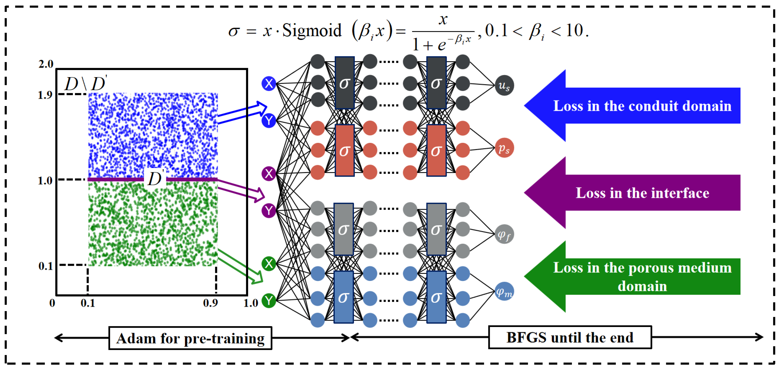
The dual adaptive neural network (DANN) algorithm is the fusion of an adaptively weighted loss function and an adaptive activation function. The solving process of the UC problem is shown in Figure 2.

For the DANN algorithm, we employ the commonly used Adam optimizer [34] to pre-training in order to accelerate convergence and obtain optimal adaptive parameters ${\beta }_i$, ${\mathit{\lambda }}_{\mathit{p}}$. The BFGS [35] is used immediately afterward until the loss function converges completely. In the Adam pre-training process, the following two optimization algorithms, gradient increase and gradient descent, are used:

$$\begin{array}{cc}\hfill {\mathit{\theta }}^{k+1}& ={\mathit{\theta }}^k-{\eta }^k{\nabla }_{\theta }J({\theta }^k,{\beta }_i^k,{\mathit{\lambda }}_p^k),\hfill \\ \hfill {\beta }_i^{k+1}& ={\beta }_i^k+{\eta }^k{\nabla }_{\theta }J({\theta }^k,{\beta }_i^k,{\mathit{\lambda }}_p^k),\hfill \\ \hfill {\mathit{\lambda }}_p^{k+1}& ={\mathit{\lambda }}_p^k+{\eta }^k{\nabla }_{{\lambda }_i}J({\theta }^k,{\beta }_i^k,{\mathit{\lambda }}_p^k).\hfill \end{array}$$

In BFGS iteration, ${\mathit{\lambda }}_p$ and ${\beta }_i$ are fixed and $\mathit{\theta }$ is used in the gradient descent algorithm until the end:

$$\begin{array}{cc}\hfill {\mathit{\theta }}^{k+1}& ={\mathit{\theta }}^k-{\alpha }^k{\nabla }_{\theta }J({\theta }^k,{\beta }_i^k,{\mathit{\lambda }}_p^k).\hfill \end{array}$$

The learning rates for the two training parts are represented by $\eta$ and $\alpha$, respectively.

Theoretically, the core of DANNs solving PDEs is the approximation of integrals using the abstract quadrature rule [10] as follows. Assume that the PDE F exists in $D^{\prime }$ and can be written in the following form:

$$F={\int }_{D^{\prime }}F\left(\overrightarrow{\mathbf{x}}\right)\mathrm{d}\overrightarrow{\mathbf{x}},$$

(25)

where $d\overrightarrow{\mathbf{x}}$ denotes the d-dimensional Lebesgue measure. To solve using a neural network, it is necessary to determine the quadrature points (sample points) ${\overrightarrow{\mathbf{x}}}_i\in D^{\prime }$ for $1\le i\le N$, where N represents the total number. Subsequently, the quadrature can be established:

$$F_N=\sum _{i+1}^N{w}_{i}F\left({\overrightarrow{\mathbf{x}}}_i\right),$$

(26)

where $w_i\in R_{+}$ is the weight of the neural network. We further assume that the quadrature error is bounded as

$$|F-F_N|\le C{N}^{-\alpha },$$

(27)

for the learning rate $\mathit{\alpha }>0$. The quadrature points and weight depend on the underlying order of the quadrature rule, and the $\mathit{\alpha }$ depends on the regularity of the function being integrated [36]. Thus, we can employ above standard quadrature rule for solving PDEs by the DANN.

4. Theoretical Analysis

In this section we obtain generalization error estimates by conditional stability analysis of the UC problem. In this way, we provide a theoretical basis for the DANN algorithm. For ease of understanding, we write $\widehat{D}=D_s\setminus D_s^{\prime }\cup D_d\setminus D_d^{\prime }$, and it has the following conditional stability.

Theorem 1.

For the dual-porosity–Navier–Stokes model, let ${\mathbf{f}}_s\in L^2\left(\widehat{D}\right)$, ${\mathrm{f}}_d\in L^2\left(\widehat{D}\right)$ and $g\in H^1\left(D^{\prime }\right)$. Let ${\mathbf{u}}_s\in H^1\left(\widehat{D}\right)$, $p_s\in L^2\left(\widehat{D}\right)$, ${\phi }_F\in H^1\left(\widehat{D}\right)$ and ${\phi }_m\in H^1\left(\widehat{D}\right)$ hold for all test functions ${\mathbf{v}}_s\in H_0^1\left(\widehat{D}\right)$, $q_s\in L_0^2\left(\widehat{D}\right)$, $v_f\in H_0^1\left(\widehat{D}\right)$ and $v_m\in H_0^1\left(\widehat{D}\right)$. We have the global stability estimate

$$\begin{array}{c}\hfill \parallel {\mathbf{u}}_s{\parallel }_{H^1\left(\widehat{D}\right)}+\parallel p_s{\parallel }_{L^2\left(\widehat{D}\right)}+\parallel {\phi }_F{\parallel }_{H^1\left(\widehat{D}\right)}+{\parallel {\phi }_m\parallel }_{H^1\left(\widehat{D}\right)}\\ \hfill ⩽C\left(\parallel {\mathbf{f}}_s{\parallel }_{L^2\left(\widehat{D}\right)}+\parallel {\mathrm{f}}_d{\parallel }_{L^2\left(\widehat{D}\right)}+{\parallel g\parallel }_{H^1\left(D^{\prime }\right)}\right),\end{array}$$

(28)

The domain $\widehat{D}$ consists of a boundary $\partial \widehat{D}=\partial D$, the boundary $\partial D^{\prime }$ and the interface ${\Gamma }_i(i=2,3)$.

Proof of Theorem 1.

Firstly, we multiply (4) by $v_m\in H_0^1\left(\widehat{D}\right)$ and (6) by $v_F\in H_0^1\left(\widehat{D}\right)$ and interface condition (8), (9). Then, integrating over $\widehat{D}$ gives the following weak form:

$$\begin{array}{cc}\hfill & {\displaystyle \frac{k_m}{\mu }}{\int }_{\widehat{D}}\nabla {\phi }_m·\nabla v_m\mathrm{d}\widehat{D}-{\displaystyle \frac{k_m}{\mu }}{\int }_{\partial D^{\prime }}\nabla {\phi }_m·{\mathbf{n}}_d·v_m\mathrm{d}\mathrm{s}+{\displaystyle \frac{k_m}{\mu }}{\int }_{\partial \widehat{D}}\nabla {\phi }_m·{\mathbf{n}}_d·v_m\mathrm{d}\mathrm{s}\hfill \\ \hfill & +{\displaystyle \frac{\sigma k_m}{\mu }}{\int }_{\widehat{D}}({\phi }_m-{\phi }_f)·v_m\mathrm{d}\widehat{D}=0,\hfill \end{array}$$

and

$$\begin{array}{cc}\hfill & {\displaystyle \frac{k_F}{\mu }}{\int }_{\widehat{D}}\nabla {\phi }_F·\nabla v_F\mathrm{d}\widehat{D}-{\displaystyle \frac{k_F}{\mu }}{\int }_{\partial D^{\prime }}\nabla {\phi }_F·{\mathbf{n}}_d·v_F\mathrm{d}\mathrm{s}+{\displaystyle \frac{k_F}{\mu }}{\int }_{\partial \widehat{D}}\nabla {\phi }_F·{\mathbf{n}}_d·v_F\mathrm{d}\mathrm{s}\hfill \\ \hfill & -{\displaystyle \frac{k_F}{\mu }}{\int }_{{\Gamma }_i}{\mathbf{u}}_s·{\mathbf{n}}_d·v_F\mathrm{d}\mathrm{s}+{\displaystyle \frac{\sigma k_m}{\mu }}{\int }_{\widehat{D}}({\phi }_F-{\phi }_m)·v_f\mathrm{d}\widehat{D}={\int }_{\widehat{D}}{\mathrm{f}}_d·v_F\mathrm{d}\widehat{D}.\hfill \end{array}$$

Let $v_F={\phi }_F$, $v_m={\phi }_m$. According to the Cauchy inequality and Poincaré inequality, we can obtain

$$\begin{array}{cc}\hfill \parallel \nabla {\phi }_m{\parallel }_{L^2\left(\widehat{D}\right)}^2+\parallel {\phi }_m{\parallel }_{L^2\left(\widehat{D}\right)}^2-\parallel {\phi }_F{\parallel }_{L^2\left(\widehat{D}\right)}{\parallel {\phi }_m\parallel }_{L^2\left(\widehat{D}\right)}& \le C_m{\parallel \nabla \mathrm{g}\parallel }_{L^2\left(D^{\prime }\right)}{\parallel {\phi }_m\parallel }_{L^2\left(\widehat{D}\right)},\hfill \\ \hfill \parallel {\phi }_m{\parallel }_{H^1\left(\widehat{D}\right)}^2+\parallel {\phi }_m{\parallel }_{L^2\left(\widehat{D}\right)}^2-\parallel {\phi }_F{\parallel }_{L^2\left(\widehat{D}\right)}{\parallel {\phi }_m\parallel }_{L^2\left(\widehat{D}\right)}& \le C_m{\parallel \mathrm{g}\parallel }_{H^1\left(D^{\prime }\right)}{\parallel {\phi }_m\parallel }_{L^2\left(\widehat{D}\right)},\hfill \\ \hfill \parallel {\phi }_m{\parallel }_{H^1\left(\widehat{D}\right)}+\parallel {\phi }_m{\parallel }_{L^2\left(\widehat{D}\right)}-{\parallel {\phi }_F\parallel }_{L^2\left(\widehat{D}\right)}& \le C_m{\parallel \mathrm{g}\parallel }_{H^1\left(D^{\prime }\right)}.\hfill \end{array}$$

(29)

$$\begin{array}{cc}\hfill & \parallel \nabla {\phi }_F{\parallel }_{L^2\left(\widehat{D}\right)}^2-\parallel {\mathbf{u}}_s{\parallel }_{L^2\left({\Gamma }_i\right)}\parallel {\phi }_F{\parallel }_{L^2\left(\widehat{D}\right)}+\parallel {\phi }_F{\parallel }_{L^2\left(\widehat{D}\right)}^2-\parallel {\phi }_m{\parallel }_{L^2\left(\widehat{D}\right)}{\parallel {\phi }_F\parallel }_{L^2\left(\widehat{D}\right)}\hfill \\ \hfill & \le C_F\left(\parallel {\mathrm{f}}_d{\parallel }_{L^2\left(\widehat{D}\right)}\parallel {\phi }_f{\parallel }_{L^2\left(\widehat{D}\right)}+{\parallel \nabla \mathrm{g}\parallel }_{L^2\left(D^{\prime }\right)}{\parallel {\phi }_F\parallel }_{L^2\left(\widehat{D}\right)}\right),\hfill \\ \hfill & \parallel {\phi }_F{\parallel }_{H^1\left(\widehat{D}\right)}^2-\parallel {\mathbf{u}}_s{\parallel }_{L^2\left({\Gamma }_i\right)}\parallel {\phi }_F{\parallel }_{L^2\left(\widehat{D}\right)}+\parallel {\phi }_F{\parallel }_{L^2\left(\widehat{D}\right)}^2-\parallel {\phi }_m{\parallel }_{L^2\left(\widehat{D}\right)}{\parallel {\phi }_f\parallel }_{L^2\left(\widehat{D}\right)}\hfill \\ \hfill & \le C_F\left(\parallel {\mathrm{f}}_d{\parallel }_{L^2\left(\widehat{D}\right)}\parallel {\phi }_F{\parallel }_{L^2\left(\widehat{D}\right)}+{\parallel \mathrm{g}\parallel }_{H^1\left(D^{\prime }\right)}{\parallel {\phi }_F\parallel }_{L^2\left(\widehat{D}\right)}\right),\hfill \\ \hfill & \parallel {\phi }_F{\parallel }_{H^1\left(\widehat{D}\right)}-\parallel {\mathbf{u}}_s{\parallel }_{L^2\left({\Gamma }_i\right)}+\parallel {\phi }_F{\parallel }_{L^2\left(\widehat{D}\right)}-{\parallel {\phi }_m\parallel }_{L^2\left(\widehat{D}\right)}\le C_f\left(\parallel {\mathrm{f}}_d{\parallel }_{L^2\left(\widehat{D}\right)}+{\parallel \mathrm{g}\parallel }_{H^1\left(D^{\prime }\right)}\right).\hfill \end{array}$$

(30)

Combining the results of (29) and (30) gives

$$\begin{array}{c}\hfill \parallel {\phi }_F{\parallel }_{H^1\left(\widehat{D}\right)}+\parallel {\phi }_m{\parallel }_{H^1\left(\widehat{D}\right)}\le C\left(\parallel {\mathrm{f}}_d{\parallel }_{L^2\left(\widehat{D}\right)}+{\parallel \mathrm{g}\parallel }_{H^1{\left(D\right)}^{\prime }}\right)+{\parallel {\mathbf{u}}_s\parallel }_{L^2\left({\Gamma }_i\right)}\end{array}$$

(31)

Then, multiplying (1) by ${\mathbf{v}}_s\in H_0^1\left(\widehat{D}\right)$ and (2) by $q\in L_0^2\left(\widehat{D}\right)$, taking the integrals similarly, we obtain the weak form for the conduit domain:

$$\begin{array}{cc}\hfill & \nu {\int }_{\widehat{D}}\nabla {\mathbf{u}}_s,\nabla {\mathbf{v}}_s\mathrm{d}\widehat{D}-\nu {\int }_{\partial D^{\prime }}\nabla {\mathbf{u}}_s·{\mathbf{n}}_d·{\mathbf{v}}_s\mathrm{d}\mathrm{s}+\nu {\int }_{\partial \widehat{D}}\nabla {\mathbf{u}}_s·{\mathbf{n}}_d·{\mathbf{v}}_s\mathrm{d}\mathrm{s}+c{({\mathbf{u}}_s,{\mathbf{u}}_s,{\mathbf{v}}_s)}_{\widehat{D}}\hfill \\ \hfill & +{\displaystyle \frac{1}{\rho }}{\int }_{{\Gamma }_i}{\phi }_F·{\mathbf{v}}_s·{\mathbf{n}}_s\mathrm{d}\mathrm{s}+\sum _{i=1}^{d-l}{\int }_{{\Gamma }_i}{\displaystyle \frac{\alpha ·\nu \sqrt{d}}{\sqrt{t_r(\Pi )}}}({\mathbf{u}}_s·{\mathit{\tau }}_i)({\mathbf{v}}_s·{\mathit{\tau }}_i)\mathrm{d}\mathrm{s}={\int }_{\widehat{D}}{\mathbf{f}}_s·{\mathbf{v}}_s\mathrm{d}\widehat{D}\hfill \\ \hfill & {\int }_{\widehat{D}}\nabla ·{\mathbf{u}}_s·q\mathrm{d}\widehat{D}=0.\hfill \end{array}$$

where the nonlinear form $c{({\mathbf{u}}_s,{\mathbf{u}}_s,{\mathbf{v}}_s)}_{\widehat{D}}:={(({\mathbf{u}}_s·\nabla ){\mathbf{u}}_s,{\mathbf{v}}_s)}_{\widehat{D}}$. Let ${\mathbf{v}}_s={\mathbf{u}}_s$. According to the nonlinear property [37], the nonlinear form can be estimated as follows:

$$\begin{array}{cc}\hfill {(({\mathbf{u}}_s·\nabla ){\mathbf{u}}_s,{\mathbf{v}}_s)}_{\widehat{D}}& \le C_N\parallel {\mathbf{u}}_s{\parallel }_{L^2\left(\widehat{D}\right)}^{{\displaystyle \frac{1}{2}}}\parallel \nabla {\mathbf{u}}_s{\parallel }_{L^2\left(\widehat{D}\right)}^{{\displaystyle \frac{1}{2}}}\parallel \nabla {\mathbf{u}}_s{\parallel }_{L^2\left(\widehat{D}\right)}{\parallel \nabla {\mathbf{u}}_s\parallel }_{L^2\left(\widehat{D}\right)}\hfill \\ \hfill & \le C_N{\parallel \nabla {\mathbf{u}}_s\parallel }_{H^1\left(\widehat{D}\right)}^3.\hfill \end{array}$$

(32)

From (10) and (11), the Cauchy inequality, (32) and the Poincaré inequality, the following conclusions can be drawn:

$$\begin{array}{cc}\hfill & \parallel \nabla {\mathbf{u}}_s{\parallel }_{L^2\left(\widehat{D}\right)}\parallel \nabla {\mathbf{u}}_s{\parallel }_{H^1\left(\widehat{D}\right)}+\parallel {\phi }_F{\parallel }_{L^2\left({\Gamma }_i\right)}\parallel {\mathbf{u}}_s{\parallel }_{H^1\left(\widehat{D}\right)}+\parallel {\mathbf{u}}_s{\parallel }_{L^2\left({\Gamma }_i\right)}{\parallel {\mathbf{u}}_s\parallel }_{H^1\left(\widehat{D}\right)}\hfill \\ \hfill & \le C_s\left(-\parallel \nabla {\mathbf{u}}_s{\parallel }_{H^1\left(\widehat{D}\right)}^3+\parallel {\mathbf{f}}_s{\parallel }_{L^2\left(\widehat{D}\right)}\parallel {\mathbf{u}}_s{\parallel }_{H^1\left(\widehat{D}\right)}+{\parallel \nabla \mathrm{g}\parallel }_{L^2\left(D^{\prime }\right)}{\parallel {\mathbf{u}}_s\parallel }_{H^1\left(\widehat{D}\right)}\right),\hfill \\ \hfill & \parallel {\mathbf{u}}_s{\parallel }_{H^1\left(\widehat{D}\right)}+\parallel {\phi }_F{\parallel }_{L^2\left({\Gamma }_i\right)}+{\parallel {\mathbf{u}}_s\parallel }_{L^2\left({\Gamma }_i\right)}\le C_s\left(-\parallel \nabla {\mathbf{u}}_s{\parallel }_{H^1\left(\widehat{D}\right)}^2+\parallel {\mathbf{f}}_s{\parallel }_{L^2\left(\widehat{D}\right)}+{\parallel \mathrm{g}\parallel }_{H^1\left(D^{\prime }\right)}\right),\hfill \\ \hfill & \parallel {\mathbf{u}}_s{\parallel }_{H^1\left(\widehat{D}\right)}+{\parallel {\mathbf{u}}_s\parallel }_{L^2\left({\Gamma }_i\right)}\le C_s\left(-\parallel \nabla {\mathbf{u}}_s{\parallel }_{H^1\left(\widehat{D}\right)}^2+\parallel {\mathbf{f}}_s{\parallel }_{L^2\left(\widehat{D}\right)}+{\parallel \mathrm{g}\parallel }_{H^1\left(D^{\prime }\right)}\right).\hfill \end{array}$$

(33)

There is, as follows, an inf-sup condition [38] for a positive constant $C_1$:

$$C_1\underset{0\ne \mathbf{v}\in {\left(H_0^1(\Omega )\right)}^d}{sup}{\displaystyle \frac{(\mathrm{div}\mathbf{v},q)}{{\parallel \mathbf{v}\parallel }_{{\left(H_0^1(\Omega )\right)}^d}}}\ge {\parallel q\parallel }_{L^2(\Omega )},\forall q\in L_0^2(\Omega ),$$

d is the dimension. Thus, according to Equation (1), there exists a $p_s\in L_0^2\left(\widehat{D}\right)$, for $\forall {\mathbf{v}}_s\in {\left(H_0^1\left(\widehat{D}\right)\right)}^d$. For a nonlinear form, we have the nonlinear property:

$$\begin{array}{cc}\hfill \parallel p_s{\parallel }_{L^2}& \le C_1\underset{{\mathbf{u}}_s\in {\left(H_0^1\left(\widehat{D}\right)\right)}^d}{sup}[{\displaystyle \frac{{\int }_{\widehat{D}}\nabla {\mathbf{u}}_s,\nabla {\mathbf{v}}_s\mathrm{d}\widehat{D}-\nu {\int }_{\partial D^{\prime }}\nabla \mathrm{g}·{\mathbf{n}}_d·\nabla {\mathbf{v}}_s\mathit{d}\partial D^{\prime }+c({\mathbf{u}}_s,{\mathbf{u}}_s,{\mathbf{v}}_s)}{\parallel {\mathbf{v}}_s{\parallel }_{H^1\left(\widehat{D}\right)}}}\hfill \\ \hfill & +{\displaystyle \frac{{\int }_{{\Gamma }_i}({\mathbf{u}}_s·{\mathit{\tau }}_i)({\mathbf{v}}_s·{\mathit{\tau }}_i)\mathrm{d}{\Gamma }_i+{\int }_{{\Gamma }_i}{\phi }_F·{\mathbf{v}}_s·{\mathbf{n}}_s\mathrm{d}{\Gamma }_i-{\int }_{\widehat{D}}{\mathbf{f}}_s,{\mathbf{v}}_s\mathrm{d}\widehat{D}}{\parallel {\mathbf{v}}_s{\parallel }_{H^1\left(\widehat{D}\right)}}}]\hfill \\ \hfill & \le C_1[{\displaystyle \frac{\parallel {\mathbf{u}}_s{\parallel }_{H^1\left(\widehat{D}\right)}\parallel {\mathbf{u}}_s{\parallel }_{H^1\left(\widehat{D}\right)}+\parallel {\phi }_F{\parallel }_{L^2\left({\Gamma }_i\right)}\parallel {\mathbf{u}}_s{\parallel }_{H^1\left(\widehat{D}\right)}+\parallel {\mathbf{u}}_s{\parallel }_{L^2\left({\Gamma }_i\right)}{\parallel {\mathbf{u}}_s\parallel }_{H^1\left(\widehat{D}\right)}}{\parallel {\mathbf{u}}_s{\parallel }_{H^1\left(\widehat{D}\right)}}}\hfill \\ \hfill & +{\displaystyle \frac{\parallel \nabla {\mathbf{u}}_s{\parallel }_{H^1\left(\widehat{D}\right)}^3-\parallel {\mathbf{f}}_s{\parallel }_{L^2\left(\widehat{D}\right)}\parallel {\mathbf{u}}_s{\parallel }_{H^1\left(\widehat{D}\right)}-{\parallel \nabla \mathrm{g}\parallel }_{L^2\left(D^{\prime }\right)}{\parallel {\mathbf{u}}_s\parallel }_{H^1\left(\widehat{D}\right)}}{\parallel {\mathbf{u}}_s{\parallel }_{H^1\left(\widehat{D}\right)}}}]\hfill \\ \hfill & \le C_1{\parallel \nabla {\mathbf{u}}_s\parallel }_{H^1\left(\widehat{D}\right)}^2.\hfill \end{array}$$

(34)

Adding up the conclusions of (31), (33) and (34) leads to

$$\begin{array}{c}\hfill \parallel {\mathbf{u}}_s{\parallel }_{H^1\left(\widehat{D}\right)}+\parallel p_s{\parallel }_{L^2\left(\widehat{D}\right)}+\parallel {\phi }_m{\parallel }_{H^1\left(\widehat{D}\right)}+{\parallel {\phi }_F\parallel }_{H^1\left(\widehat{D}\right)}\\ \hfill \le C\left(\parallel {\mathrm{f}}_d{\parallel }_{L^2\left(\widehat{D}\right)}+\parallel {\mathbf{f}}_s{\parallel }_{L^2\left(\widehat{D}\right)}+{\parallel \mathrm{g}\parallel }_{H^1\left(D^{\prime }\right)}\right).\end{array}$$

(35)

□

Theorem 2.

For the triple-porosity–Navier–Stokes model, let ${\mathbf{f}}_s\in L^2\left(\widehat{D}\right)$, ${\mathrm{f}}_d\in L^2\left(\widehat{D}\right)$ and $g\in H^1\left(D^{\prime }\right)$. Let ${\mathbf{u}}_s\in H^1\left(\widehat{D}\right)$, $p_s\in L^2\left(\widehat{D}\right)$, ${\phi }_F\in H^1\left(\widehat{D}\right)$, ${\phi }_f\in H^1\left(\widehat{D}\right)$ and ${\phi }_m\in H^1\left(\widehat{D}\right)$ hold for all test functions ${\mathbf{v}}_s\in H_0^1\left(\widehat{D}\right)$, $q_s\in L_0^2\left(\widehat{D}\right)$, $v_f\in H_0^1\left(\widehat{D}\right)$ and $v_m\in H_0^1\left(\widehat{D}\right)$. We have the global stability estimate

$$\begin{array}{c}\hfill \parallel {\mathbf{u}}_s{\parallel }_{H^1\left(\widehat{D}\right)}+\parallel p_s{\parallel }_{L^2\left(\widehat{D}\right)}+\parallel {\phi }_F{\parallel }_{H^1\left(\widehat{D}\right)}+\parallel {\phi }_f{\parallel }_{H^1\left(\widehat{D}\right)}+{\parallel {\phi }_m\parallel }_{H^1\left(\widehat{D}\right)}\\ \hfill ⩽C\left(\parallel {\mathbf{f}}_s{\parallel }_{L^2\left(\widehat{D}\right)}+\parallel {\mathrm{f}}_d{\parallel }_{L^2\left(\widehat{D}\right)}+{\parallel g\parallel }_{H^1\left(D^{\prime }\right)}\right),\end{array}$$

(36)

The proof of Theorem 2 is very similar to Theorem 1 and is easily obtained. For the generalization error of each physical quantity, we set ${\mathbf{u}}_s^{*},p_s^{*},{\phi }_m^{*}$, ${\phi }_F^{*}$ and ${\phi }_f^{*}$ as the neural network solution using the DANN. ${\mathrm{f}}_d^{*}$ and ${\mathbf{f}}_s^{*}$ are the right terms satisfied by the neural network solution. The observational data approximated by the DANN is denoted by $g^{*}$. Define the error ${\epsilon }_s={\mathbf{u}}_s-{\mathbf{u}}_s^{*}\in H^1\left(\widehat{D}\right)$, ${\epsilon }_p=p_s-p_s^{*}\in L^2\left(\widehat{D}\right)$, ${\epsilon }_m={\phi }_m-{\phi }_m^{*}\in H^1\left(\widehat{D}\right)$, ${\epsilon }_F={\phi }_F-{\phi }_F^{*}\in H^1\left(\widehat{D}\right)$ and ${\epsilon }_f={\phi }_f-{\phi }_f^{*}\in H^1\left(\widehat{D}\right)$.

Remark 1.

According to the conclusion of Theorems 1 and 2, the global generalization error between the analytical solution and the neural network solution will also be satisfied:

$$\begin{array}{cc}\hfill {\parallel \epsilon \parallel }_{H^1\left(\widehat{D}\right)}& =\parallel {\epsilon }_s{\parallel }_{H^1\left(\widehat{D}\right)}+\parallel {\epsilon }_p{\parallel }_{L^2\left(\widehat{D}\right)}+\parallel {\epsilon }_m{\parallel }_{H^1\left(\widehat{D}\right)}+\parallel {\epsilon }_F{\parallel }_{H^1\left(\widehat{D}\right)}+{\parallel {\epsilon }_f\parallel }_{H^1\left(\widehat{D}\right)}\hfill \\ & \le C\left(\parallel {\mathrm{f}}_d-{\mathrm{f}}_d^{*}{\parallel }_{L^2\left(\widehat{D}\right)}+\parallel {\mathbf{f}}_s-{\mathbf{f}}_s^{*}{\parallel }_{L^2\left(\widehat{D}\right)}+{\parallel \mathrm{g}-{\mathrm{g}}^{*}\parallel }_{H^1\left(D^{\prime }\right)}\right).\hfill \end{array}$$

(37)

The global generalization error is defined by $\epsilon \in H^1\left(\widehat{D}\right)$.

According to recent papers [20], the generalization error estimate is also determined by the training error $\mathcal{E}$ defined from the loss function (24) as follows:

$$\begin{array}{cc}\hfill \mathcal{E}& :={\left(J_{{\Omega }_s}(\mathbf{x};\mathit{\theta },{\mathit{\lambda }}_{\mathit{s}})\right)}^{{\displaystyle \frac{1}{2}}}+{\left(J_{\partial {\Omega }_s}(\mathbf{x};\mathit{\theta },{\mathit{\lambda }}_{\mathit{bs}})\right)}^{{\displaystyle \frac{1}{2}}}+{\left(J_{{\Omega }_d}(\mathbf{x};\mathit{\theta },{\mathit{\lambda }}_{\mathit{d}})\right)}^{{\displaystyle \frac{1}{2}}}\hfill \\ & +{\left(J_{\partial {\Omega }_d}(\mathbf{x};\mathit{\theta },{\mathit{\lambda }}_{\mathit{bd}})\right)}^{{\displaystyle \frac{1}{2}}}+{\left(J_{\Gamma }(\mathbf{x};\mathit{\theta },{\mathit{\lambda }}_{\mathit{i}})\right)}^{{\displaystyle \frac{1}{2}}}\hfill \end{array}$$

(38)

The training error $\mathcal{E}$ can be easily computed from the loss function at the end of the training. Thus, we can estimate the global generalization error in the following result.

Theorem 3.

According to the abstract quadrature formulas, the global generalization error $\parallel \epsilon \parallel$ can be further estimated by the following form:

$$\begin{array}{cc}\hfill \parallel \epsilon \parallel & \le C\left(\mathcal{E}+C_{int}{N}_{int}^{-\alpha }\right).\hfill \end{array}$$

(39)

C and $C_{int}$ are non-negative constants, and $N_{int}$ denotes the total number of sample points in the domain $D^{\prime }$.

Proof of Theorem 3.

According to Remark 1, the $\parallel \epsilon \parallel$ can be constrained from training error $\mathcal{E}$ and the quadrature error (27) to be

$$\begin{array}{cc}\hfill \parallel \epsilon \parallel & \le C\left(\parallel {\mathrm{f}}_d-{\mathrm{f}}_d^{*}{\parallel }_{L^2\left(\widehat{D}\right)}+\parallel {\mathbf{f}}_s-{\mathbf{f}}_s^{*}{\parallel }_{L^2\left(\widehat{D}\right)}+{\parallel \mathrm{g}-{\mathrm{g}}^{*}\parallel }_{H^1\left(D^{\prime }\right)}\right)\hfill \\ \hfill & \le C\left(\mathcal{E}+C_{f_s}{N}_{f_s}^{-\mathit{\alpha }}+C_{f_d}{N}_{f_d}^{-\mathit{\alpha }}+C_{\Gamma }{N}_{\Gamma }^{-\mathit{\alpha }}+C_{bo{u}_s}{N}_{bo{u}_s}^{-\mathit{\alpha }}+C_{bo{u}_d}{N}_{bo{u}_d}^{-\mathit{\alpha }}\right)\hfill \\ \hfill & \le C\left(\mathcal{E}+C_{int}{N}_{int}^{-\mathit{\alpha }}\right),\hfill \end{array}$$

where $N_{int}=max\left(\{N_{f_s},N_{f_d},N_{\Gamma },N_{bo{u}_s},N_{bo{u}_d}\}\right)$. □

Remark 2.

Theorem 3 explains the mechanism for solving the UC problem using the DANN because it decomposes the source of error into the following parts:

• The DANN algorithm uses an adaptively weighted loss function. This makes training adequate, meaning that the training error $\mathcal{E}$ is small enough. We show the value of loss and plot the adaptively weighted value in the loss in the experiments in Section 5.
• The DANN algorithm uses an adaptive activation function. It excellently performs adaptive computation for different physical quantities. In Section 5, the results of the adaptive Swish activation function are preferred to Sigmoid and Tanh.
• The error estimation in Theorem 3 relies on the conditional stability for the UC problem. Thus, the generalization error achieves an efficient approximation through DANN and the conditional stability of the PDEs.

5. Numerical Experiment

In this section, we conduct numerical experiments on the two types of free-flow coupled porous medium models mentioned in Section 2. We select the network parameters for the DANN algorithm as summarized in

Table 1. The parameters of the neural network.

${\mathit{N}}_{\mathit{bs}}={\mathit{N}}_{\mathit{bd}}$	${\mathit{N}}_{\mathit{i}}$	${\mathit{N}}_{\mathit{s}}={\mathit{N}}_{\mathit{d}}$	${\mathit{N}}_{\mathit{N}}$	$\mathit{\eta }$	$\mathit{\alpha }$	Max Iterations
800	800	4000	32	$0.001$	$1\times {10}^{-8}$	40,000

, where $N_N$ denotes the number of neurons in each hidden layer. The learning rate for Adam pre-training is $\eta$, and the BFGS iteration is chosen to be $\alpha$. And $N_i(i=bs,bd,i,s,d)$ denotes the number of observational data at the boundary, the interface and the interior, respectively. Notably, for ease of understanding and training, all learnable parameters ${\mathit{\lambda }}_i$ and ${\beta }_i$ are initialized to 1. The numerical experiment in this section is based on the Tensorflow 1.14, the code is written in Python 3.7 and the CPU is an Intel(R) Core(TM) i7-12700H.

5.1. Dual-Porosity–Navier–Stokes Model with Analytical Solution

In this example, the computational domain D is composed of two subdomains. The free-flow domain $D_s=[0,1]\times [1,2]$, and the porous media domain $D_d=[0,1]\times [0,1]$. The interface $\Gamma =[0,1]\times \left\{1\right\}$. For computational simplicity, all physical parameters, including $\nu$, $\mu$, $\sigma$, $k_m$, $k_f$, $\rho$ and $\alpha$, are set to 1. The spatial dimension is $d=2$. The source term in the dual-porosity–Navier–Stokes model is defined by the following analytical solution:

$$\begin{array}{cc}\hfill {\mathbf{u}}_s& =\left((x^2{(y-1)}^2+y),(-{\displaystyle \frac{2}{3}}x{(y-1)}^3+2-\pi sin\left(\pi x\right))\right),\hfill \\ \hfill p_s& =(2-\pi sin\left(\pi x\right))sin({\displaystyle \frac{\pi }{2}}y),\hfill \\ \hfill {\phi }_f& =\left(2-\pi sin\left(\pi x\right)\right)\left(1-y-cos\left(\pi y\right)\right),\hfill \\ \hfill {\phi }_m& =(2-\pi sin(\pi x\left)\right)cos\left(\pi \right(1-y\left)\right).\hfill \end{array}$$

In the UC problem, observational data can only be obtained from $D_s^{\prime }=[0.1,0.9]\times [1,1.9]$ and $D_d^{\prime }=[0.1,0.9]\times [0.1,1]$, as shown in Figure 3 Left. The data of the boundary and near the boundary, shown in Figure 3 Right, are unknown.

At the end of the training, the adaptively weighted values are shown in Figure 4, and the values in the adaptive activation function are ${\beta }_s=1.43$, ${\beta }_p=1.58$, ${\beta }_F=1.21$ and ${\beta }_m=1.14$, respectively.

First, we perform ablation experiments to prove that the DANN algorithm can obtain accurate results. In

Table 2. Loss functions and $L^2$ error results for different methods. The best results are highlighted in bold.

	Non-Adaptive	Adaptive Swish	Adaptively Weighted	DANN
Loss	$5.16\times {10}^{-6}$	$4.02\times {10}^{-6}$	$4.72\times {10}^{-6}$	$\mathbf{3}.\mathbf{97}\times {\mathbf{10}}^{-\mathbf{6}}$
$\parallel {\mathbf{u}}_{\mathit{s}}-{\mathbf{u}}_{\mathit{s}}^{*}{\parallel }_{L^2}$	$1.76\times {10}^{-6}$	$2.21\times {10}^{-6}$	$1.81\times {10}^{-6}$	$\mathbf{1}.\mathbf{20}\times {\mathbf{10}}^{-\mathbf{6}}$
$\parallel p_s-p_s^{*}{\parallel }_{L^2}$	$6.46\times {10}^{-5}$	$6.67\times {10}^{-5}$	$5.03\times {10}^{-5}$	$\mathbf{4}.\mathbf{98}\times {\mathbf{10}}^{-\mathbf{5}}$
$\parallel {\phi }_F-{\phi }_F^{*}{\parallel }_{L^2}$	$5.20\times {10}^{-6}$	$3.87\times {10}^{-6}$	$2.36\times {10}^{-6}$	$\mathbf{2}.\mathbf{29}\times {\mathbf{10}}^{-\mathbf{6}}$
$\parallel {\phi }_m-{\phi }_m^{*}{\parallel }_{L^2}$	$4.28\times {10}^{-4}$	$4.14\times {10}^{-4}$	$1.03\times {10}^{-6}$	$\mathbf{5}.\mathbf{77}\times {\mathbf{10}}^{-\mathbf{7}}$

, “Non-adaptive” refers to the algorithm that has no adaptive techniques applied. “Adaptive Swish” and “Adaptively weighted” denote the use of the adaptive algorithms in Section 3.1 and Section 3.2 alone, respectively. To ensure that changes are unique, both “non-adaptive” and “adaptive weighting” use the standard Swish activation function of ${\beta }_i=1$. And each method employs three hidden layers.

From the results of solving the UC problem in Table 2, the DANN algorithm obtains the majority of the best results. The second-best results are close to the best results. Furthermore, the DANN algorithm can obtain the minimum loss function value, which means it can achieve the minimum training error. According to Theorem 3, the DANN algorithm can also achieve the optimal error.

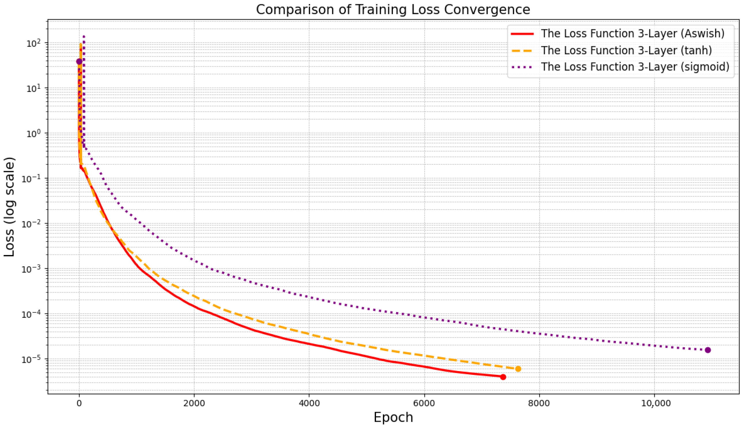
Similar to [29], we discuss the advantages of the adaptive Swish activation function compared to the Sigmoid and Tanh activation functions commonly used to solve PDEs as follows. Figure 5 shows the loss function trained using three hidden layers. “ASwish” stands for using the adaptive Swish activation function. The use of adaptive Swish results in the minimum loss function. According to Theorem 3, this indicates that its error is optimal.

To ensure that only the activation function changes, the loss function uses the adaptively weighted loss described in Section 3.1. Considering the accuracy of solving the UC problem of the dual-porosity–Naiver–Stokes model,

Table 3. The $L^1$ and $L^2$ error of each quantity to be solved in the UC problem using three hidden layers. The best results are highlighted in bold. Here, ${\epsilon }_s={\mathbf{u}}_s-{\mathbf{u}}_s^{*}$, ${\epsilon }_p=p_s-p_s^{*}$, ${\epsilon }_m={\phi }_m-{\phi }_m^{*}$ and ${\epsilon }_F={\phi }_F-{\phi }_F^{*}$.

	DANN (Adaptive Swish)		Tanh		Sigmoid
	${\mathit{L}}^{\mathbf{1}}$ Error	${\mathit{L}}^{\mathbf{2}}$ Error	${\mathit{L}}^{\mathbf{1}}$ Error	${\mathit{L}}^{\mathbf{2}}$ Error	${\mathit{L}}^{\mathbf{1}}$ Error	${\mathit{L}}^{\mathbf{2}}$ Error
$\parallel {\epsilon }_s\parallel$	$\mathbf{7}.\mathbf{01}\times {\mathbf{10}}^{-\mathbf{7}}$	$\mathbf{1}.\mathbf{76}\times {\mathbf{10}}^{-\mathbf{6}}$	$1.32\times {10}^{-6}$	$3.01\times {10}^{-6}$	$1.53\times {10}^{-6}$	$4.17\times {10}^{-6}$
$\parallel {\epsilon }_p\parallel$	$\mathbf{2}.\mathbf{72}\times {\mathbf{10}}^{-\mathbf{5}}$	$\mathbf{6}.\mathbf{46}\times {\mathbf{10}}^{-\mathbf{5}}$	$4.72\times {10}^{-5}$	$1.02\times {10}^{-4}$	$7.27\times {10}^{-5}$	$1.60\times {10}^{-4}$
$\parallel {\epsilon }_F\parallel$	$\mathbf{1}.\mathbf{03}\times {\mathbf{10}}^{-\mathbf{6}}$	$\mathbf{3}.\mathbf{20}\times {\mathbf{10}}^{-\mathbf{6}}$	$1.61\times {10}^{-6}$	$4.17\times {10}^{-6}$	$1.99\times {10}^{-6}$	$4.24\times {10}^{-6}$
$\parallel {\epsilon }_m\parallel$	$\mathbf{7}.\mathbf{13}\times {\mathbf{10}}^{-\mathbf{7}}$	$\mathbf{1}.\mathbf{77}\times {\mathbf{10}}^{-\mathbf{6}}$	$1.34\times {10}^{-6}$	$4.18\times {10}^{-6}$	$8.73\times {10}^{-7}$	$3.21\times {10}^{-6}$

shows the $L^1$ and $L^2$ error by using different activation functions. From the results, the DANN algorithm obtains the optimal $L^1$ and $L^2$ error. Based on the above results, the adaptive Swish activation function is the most suitable.

Figure 6 and Figure 7 illustrate the analytical solution from observational data and the neural network solution of the DANN algorithm using three hidden layers. The results clearly show that the DANN algorithm is still able to compute the solution over the entire domain with incomplete data.

To confirm the accuracy of the DANN algorithm in an unknown domain, we randomly selected unknown points, as shown in Figure 3 Right, to verify the error between the neural network solution and the analytical solution. The errors between them are almost all 0. The results in Figure 8 prove that the DANN algorithm successfully solves the UC problem of the dual-porosity–Navier–Stokes model and extends the prediction range effectively.

In free-flow coupled porous media models, investigating fluid flow within complex domains is also crucial [39]. Therefore, we examine the proposed DANN algorithm’s ability to solve the UC problem within complex regions. The specific complex domain design is illustrated in Figure 9 Left.

After training, the values of $lambd{a}_i$ in the adaptively weighted loss are as shown in Figure 9 Right. The values of ${\beta }_s=1.20,{\beta }_p=1.16,{\beta }_F=1.41$ and ${\beta }_m=1.43$ are used in the adaptive activation function. The analytical solution, the solutions computed by the DANN and the error between them are plotted in Figure 10. The neural network solution is identical to that in Figure 7. It can be observed that the DANN approach can also solve the UC problem in complex domains, effectively recovering information about solutions in unknown domains.

5.2. Cavity Flow Test of Dual-Porosity–Navier–Stokes Model

Based on recent literature [40,41,42], we explore the flow of free-flowing fluids without relying on analytical solutions. Specifically, we examine the case where fluids in a coupled porous medium model flow through an interface. Bo et al. [42] use the non-equilibrium extrapolation scheme to set boundary conditions for the experiment and simulate the flow patterns of the fluid.

In this subsection, the cavity flow simulations of the dual-porosity–Navier–Stokes model are considered under the UC problem. Let computational domain $D_s=[0,1]\times [1,1.25]$, $D_d=[0,1]\times [0,1]$. The observational domain $D_d^{\prime }=[0.1,0.9]\times [0.1,1]$, as shown in Figure 11 Left. And the condition imposed on the free-flow domain is as follows:

$$\begin{array}{c}\hfill {\mathbf{u}}_s=\left[sin\left(\pi x\right),0\right],\end{array}$$

The Delicacy condition is applied at the boundary [40,41]. The pressure in the major fracture is set to ${\phi }_F=0$, and the pressure in the matrix is ${\phi }_m=0$. The remaining parameters, including $d=2$, $\nu$, $\mu$, $\sigma$, $k_m$, $k_f$, $\rho$ and $\alpha$, are all assumed to be 1. The external force terms ${\mathbf{f}}_s$ and ${\mathrm{f}}_d$ are both equal to 0.

In this experiment, the neural network uses three hidden layers. At the end of pre-training, the visualization of the results for ${\mathit{\lambda }}_{\mathit{p}}$ in the adaptively weighted loss function is shown in Figure 11 Right. And ${\beta }_s=1.14$, ${\beta }_p=1.09$, ${\beta }_F=1.02$ and ${\beta }_m=1.02$ in the adaptive Swish activation function.

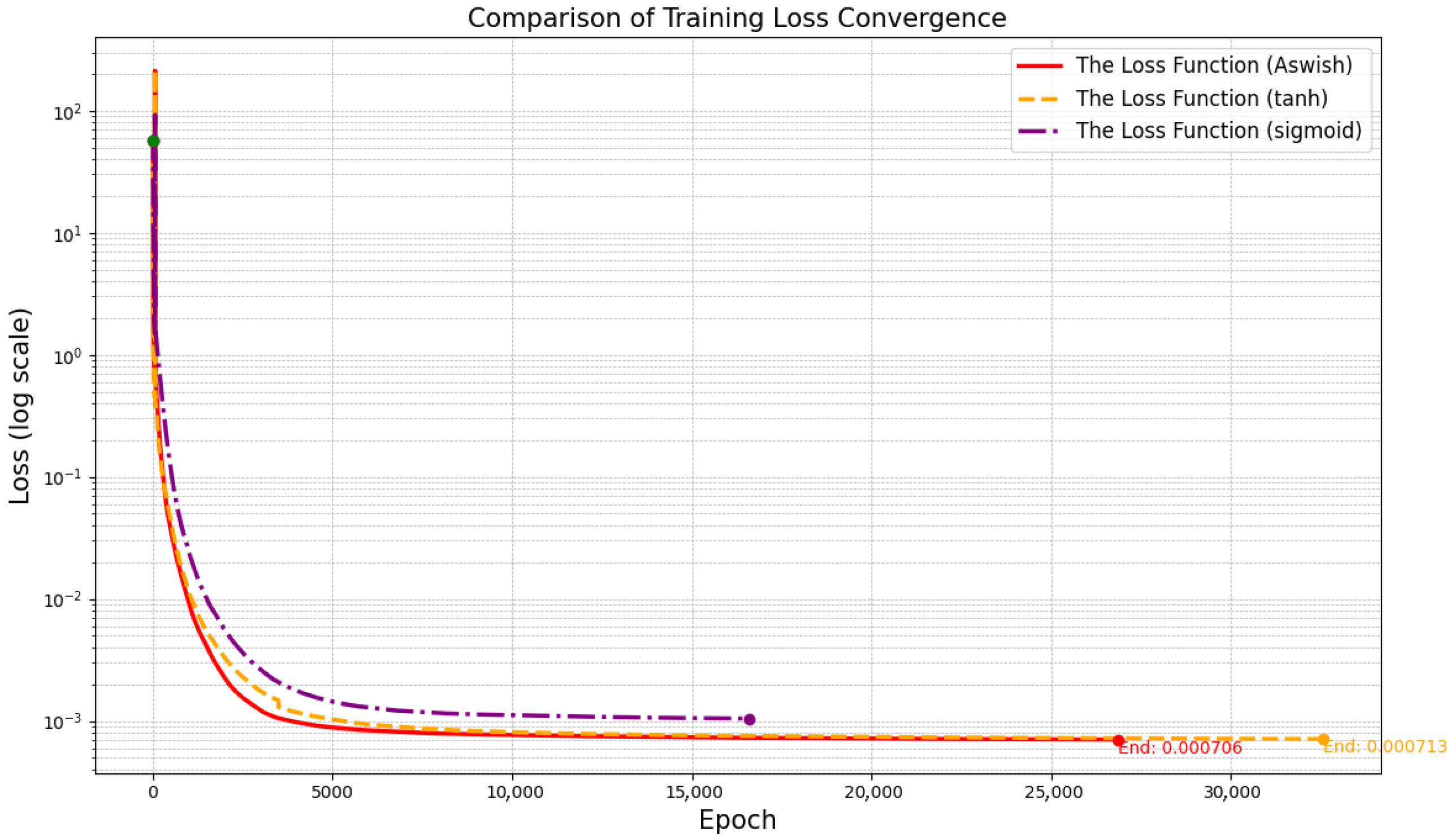
The simulation results are shown in Figure 12, which are similar to the experimental results in paper [40]. In Figure 13, the DANN algorithm using the adaptive Swish activation function can also obtain the minimum loss function value in experiments without analytical solutions. In other words, it can obtain the optimal results.

5.3. Triple-Porosity–Navier–Stokes Model with Analytical Solution

In this subsection, we discuss the UC problem of the triple-porosity–Navier–Stokes model. Let $D_s=[0,1]\times [1,2]$, $D_s=[0,1]\times [0,1]$ and the interface $\Gamma =[0,1]\times \left\{1\right\}$. We set following analytical solution:

$$\begin{array}{cc}\hfill {\mathbf{u}}_s& =\left((x^2{(y-1)}^2+y),(-{\displaystyle \frac{2}{3}}x{(y-1)}^3+2-\pi sin\left(\pi x\right))\right),\hfill \\ \hfill p_s& =(2-\pi sin\left(\pi x\right))sin({\displaystyle \frac{\pi }{2}}y),\hfill \\ \hfill {\phi }_F& =\left(2-\pi sin\left(\pi x\right)\right)\left(1-y-cos\left(\pi y\right)\right),\hfill \\ \hfill {\phi }_f& =(2-\pi sin(\pi x\left)\right)cos\left(\pi \right(1-y\left)\right),\hfill \\ \hfill {\phi }_m& =(2-\pi sin\left(\pi x\right))sin(3y^3-2y^2).\hfill \end{array}$$

All the parameters $k_i(i=F,f,m),\sigma ,{\sigma }^{*},\mu ,\rho ,\eta ,\nu$ and $\alpha$ are supposed to be 1. Further in the UC problem, the observational domain $D_s^{\prime }=[0.1,0.9]\times [1,1.9]$ and $D_d^{\prime }=[0.1,0.9]\times [0.1,1]$. The training points obtained from the observational domain are shown in Figure 3 Left. The adaptively weighted values are shown in Figure 14. The values of ${\beta }_i$ for the adaptive Swish are ${\beta }_s=1.27$, ${\beta }_p=1.41$, ${\beta }_F=1.53$, ${\beta }_f=1.36$ and ${\beta }_m=1.13$ with the neural network using three hidden layers.

Similar to Section 5.1, we also discuss the reason for choosing the adaptive Swish activation function in the triple-porosity–Navier–Stokes model. Based on the comparative results in Figure 15 and the error results in

Table 4. The $L^1$ and $L^2$ error of each quantity to be solved in the UC problem using three hidden layers. The best results are highlighted in bold. Here, ${\epsilon }_s={\mathbf{u}}_s-{\mathbf{u}}_s^{*}$, ${\epsilon }_p=p_s-p_s^{*}$, ${\epsilon }_m={\phi }_m-{\phi }_m^{*}$, ${\epsilon }_F={\phi }_f-{\phi }_f^{*}$ and ${\epsilon }_F={\phi }_F-{\phi }_F^{*}$.

	DANN (Adaptive Swish)		Tanh		Sigmoid
	${\mathit{L}}^{\mathbf{1}}$ Error	${\mathit{L}}^{\mathbf{2}}$ Error	${\mathit{L}}^{\mathbf{1}}$ Error	${\mathit{L}}^{\mathbf{2}}$ Error	${\mathit{L}}^{\mathbf{1}}$ Error	${\mathit{L}}^{\mathbf{2}}$ Error
$\parallel {\epsilon }_s\parallel$	$\mathbf{8}.\mathbf{01}\times {\mathbf{10}}^{-\mathbf{7}}$	$\mathbf{1}.\mathbf{99}\times {\mathbf{10}}^{-\mathbf{6}}$	$9.16\times {10}^{-7}$	$2.28\times {10}^{-6}$	$9.80\times {10}^{-7}$	$2.88\times {10}^{-6}$
$\parallel {\epsilon }_p\parallel$	$\mathbf{2}.\mathbf{43}\times {\mathbf{10}}^{-\mathbf{5}}$	$\mathbf{4}.\mathbf{69}\times {\mathbf{10}}^{-\mathbf{5}}$	$3.13\times {10}^{-5}$	$7.07\times {10}^{-5}$	$3.59\times {10}^{-5}$	$8.23\times {10}^{-5}$
$\parallel {\epsilon }_F\parallel$	$\mathbf{1}.\mathbf{45}\times {\mathbf{10}}^{-\mathbf{6}}$	$\mathbf{4}.\mathbf{18}\times {\mathbf{10}}^{-\mathbf{6}}$	$2.37\times {10}^{-6}$	$1.08\times {10}^{-5}$	$2.89\times {10}^{-6}$	$1.10\times {10}^{-5}$
$\parallel {\epsilon }_f\parallel$	$\mathbf{4}.\mathbf{21}\times {\mathbf{10}}^{-\mathbf{7}}$	$\mathbf{1}.\mathbf{84}\times {\mathbf{10}}^{-\mathbf{6}}$	$9.72\times {10}^{-7}$	$3.29\times {10}^{-6}$	$1.02\times {10}^{-6}$	$4.93\times {10}^{-6}$
$\parallel {\epsilon }_m\parallel$	$\mathbf{4}.\mathbf{34}\times {\mathbf{10}}^{-\mathbf{6}}$	$\mathbf{7}.\mathbf{36}\times {\mathbf{10}}^{-\mathbf{6}}$	$5.45\times {10}^{-6}$	$8.94\times {10}^{-6}$	$5.31\times {10}^{-6}$	$8.81\times {10}^{-6}$

, the DANN algorithm using the adaptive Swish activation function proposed in this paper obtains optimality in both the loss function, $L^1$ and $L^2$ error.

Figure 16 illustrates the information of the analytical solution on the observational domain. Figure 17 plots the neural network solution for the computational domain solved by the DANN algorithm. It shows that the DANN algorithm effectively solves the UC problem and successfully extends the prediction range.

Similar to Figure 3 Right, we randomly selected test points to verify the accuracy of the DANN in an unknown domain. From Figure 18, it can be judged that the DANN algorithm has successfully expanded the range of predictions.

5.4. Triple-Porosity–Navier–Stokes Model in 3D

In the 3D experiment, let computational domain $D=[0,1]\times [0,1]\times [-0.25,0.75]$. The observational domain $D^{\prime }=[0.1,0.9]\times [0.1,0.9]\times [-0.15,0.65]$ with $D_d^{\prime }=\{(x,y,z)\in D|z⩾0\}$ and $D_s^{\prime }=\{(x,y,z)\in D|z⩽0\}$ and $\Gamma =\left\{\right(x,y,z)\in D|z=0\}$. The distribution of observational data is shown in Figure 19 Left.

We utilize the analytical solution in [37] as below. And the physical parameters of this model are also simply set, i.e., $k_i(i=F,f,m),\sigma ,{\sigma }^{*},\mu ,\rho ,\eta ,\nu$ and $\alpha$ are supposed to be 1.

$$\begin{array}{cc}\hfill p_m& =-z+exp\left(z\right)sin\left(xy\right)cos\left(z\right),\hfill \\ \hfill p_f& =-z+exp\left(z\right)sin\left(xy\right)cos\left(z\right),\hfill \\ \hfill p_F& =-z+(-x^2-y^2+8)sin\left(xy\right)cos\left(z\right),\hfill \\ \hfill {\mathbf{u}}_c& =\left[\begin{array}{c}(2xsin\left(xy\right)+y(x^2+y^2-8)cos\left(xy\right))\\ (2ysin\left(xy\right)+x(x^2+y^2-8)cos\left(xy\right))\\ 1+((x^2+y^2)(x^2+y^2-8)sin\left(xy\right)-4sin\left(xy\right)-8xycos\left(xy\right))\end{array}\right],\hfill \\ \hfill p_s& =(-16xycos\left(xy\right)+(x^2+y^2+z^2-8)(2x^2+2y^2+2z^2-1)sin\left(xy\right)-8sin\left(xy\right)).\hfill \end{array}$$

In this experiment, the neural network uses three hidden layers. At the end of training, the values in the adaptive activation function are ${\beta }_s=1.32$, ${\beta }_p=1.21$, ${\beta }_F=1.56$, ${\beta }_f=1.17$ and ${\beta }_m=1.19$. The adaptively weighted values are shown in Figure 19 Right. The results of the 3D UC problem are shown in Figure 20. The DANN algorithm brilliantly solves the UC problem in 3D and effectively extends the prediction range. Errors are also within acceptable limits.

The loss function is adaptively weighted from Section 3.1. We demonstrate through Figure 21 and

Table 5. The $L^1$ and $L^2$ error of each quantity to be solved in the 3D UC problem using three hidden layers. The best results are highlighted in bold. Here, ${\epsilon }_s={\mathbf{u}}_s-{\mathbf{u}}_s^{*}$, ${\epsilon }_p=p_s-p_s^{*}$, ${\epsilon }_m={\phi }_m-{\phi }_m^{*}$, ${\epsilon }_F={\phi }_f-{\phi }_f^{*}$ and ${\epsilon }_F={\phi }_F-{\phi }_F^{*}$.

	DANN (Adaptive Swish)		Tanh		Sigmoid
	${\mathit{L}}^{\mathbf{1}}$ Error	${\mathit{L}}^{\mathbf{2}}$ Error	${\mathit{L}}^{\mathbf{1}}$ Error	${\mathit{L}}^{\mathbf{2}}$ Error	${\mathit{L}}^{\mathbf{1}}$ Error	${\mathit{L}}^{\mathbf{2}}$ Error
$\parallel {\epsilon }_s\parallel$	$\mathbf{1}.\mathbf{30}\times {\mathbf{10}}^{-\mathbf{4}}$	$\mathbf{1}.\mathbf{76}\times {\mathbf{10}}^{-\mathbf{4}}$	$2.76\times {10}^{-4}$	$3.28\times {10}^{-4}$	$1.31\times {10}^{-3}$	$1.78\times {10}^{-3}$
$\parallel {\epsilon }_p\parallel$	$\mathbf{5}.\mathbf{68}\times {\mathbf{10}}^{-\mathbf{4}}$	$\mathbf{8}.\mathbf{47}\times {\mathbf{10}}^{-\mathbf{4}}$	$6.29\times {10}^{-4}$	$1.07\times {10}^{-3}$	$5.27\times {10}^{-3}$	$7.74\times {10}^{-3}$
$\parallel {\epsilon }_F\parallel$	$\mathbf{1}.\mathbf{04}\times {\mathbf{10}}^{-\mathbf{6}}$	$\mathbf{1}.\mathbf{06}\times {\mathbf{10}}^{-\mathbf{5}}$	$2.81\times {10}^{-6}$	$1.53\times {10}^{-5}$	$1.16\times {10}^{-5}$	$1.42\times {10}^{-5}$
$\parallel {\epsilon }_f\parallel$	$\mathbf{1}.\mathbf{68}\times {\mathbf{10}}^{-\mathbf{6}}$	$\mathbf{2}.\mathbf{65}\times {\mathbf{10}}^{-\mathbf{6}}$	$2.47\times {10}^{-6}$	$4.07\times {10}^{-6}$	$7.47\times {10}^{-6}$	$1.07\times {10}^{-5}$
$\parallel {\epsilon }_m\parallel$	$\mathbf{1}.\mathbf{29}\times {\mathbf{10}}^{-\mathbf{6}}$	$\mathbf{2}.\mathbf{19}\times {\mathbf{10}}^{-\mathbf{6}}$	$1.48\times {10}^{-6}$	$3.38\times {10}^{-6}$	$4.07\times {10}^{-6}$	$5.88\times {10}^{-6}$

that adaptive Swish is also optimal in 3D. The best results are obtained using the DANN algorithm with adaptive Swish. It also proves that the DANN is the most appropriate algorithm for solving the UC problem.

We select test points from $D\setminus D^{\prime }$, as shown in Figure 19 Left. From the error in the unknown domain in Figure 22, it can be determined that the DANN algorithm can effectively solve the UC problem in 3D.

6. Conclusions

In this paper, we propose a dual adaptive neural network (DANN) algorithm for solving free-flow coupled porous media models under the unique continuation (UC) problem. The proposed algorithm is applicable to both the UC problem and general forward problem for solving PDEs. The experimental results in this paper show that the DANN algorithm achieves performance in the UC problem of two classical free-flow coupled porous media models. The DANN algorithm combines adaptively weighted loss and adaptive activation function. Numerical experiments can verify that the more complexity the model is faced with, the more obvious the accuracy of the solution obtained by the DANN algorithm. In the theoretical analysis, we provide a generalization error estimate for the UC problem and explain the rationale behind the feasibility of solving this problem using neural network. Future research directions include the following:

• Explore the integration of combined activation functions (e.g., Aswish, Tanh and Sigmoid) within an adaptive framework to further enhance the performance and flexibility of the network.
• Investigate unique continuation under time-dependent problems and propose neural network or machine learning algorithms that outperform the traditional Kalman filter method.
• Explore whether deep operator networks (DeepONets) possess the capability to solve the UC problem and compare their performance with that of physics-informed neural networks (PINNs).
• Discuss the application of the UC problem in practical real-world scenarios. We will actively explore how to incorporate real observational data into our framework to further validate the practicality of the proposed method beyond analytical solution benchmarks.

References

1. Gao, L.; Li, J. A decoupled stabilized finite element method for the dual–porosity–Navier–Stokes fluid flow model arising in shale oil. Numer. Methods Partial Differ. Equ. 2021, 37, 2357–2374. [Google Scholar] [CrossRef]
2. Kashani, E.; Mohebbi, A.; Monfared, A.E.F.; de Vries, E.T.; Raoof, A. Lattice Boltzmann simulation of dissolution patterns in porous media: Single porosity versus dual porosity media. Adv. Water Resour. 2024, 188, 104712. [Google Scholar] [CrossRef]
3. Yadav, M.P.; Agarwal, R.; Purohit, S.D.; Kumar, D.; Suthar, D.L. Groundwater flow in karstic aquifer: Analytic solution of dual–porosity fractional model to simulate groundwater flow. Appl. Math. Sci. Eng. 2022, 30, 598–608. [Google Scholar] [CrossRef]
4. Li, J.; Gao, Z.Y.; Cao, L.L.; Chen, Z.X. A local parallel fully mixed finite element method for superposed fluid and porous layers. J. Comput. Appl. Math. 2026, 472, 116798. [Google Scholar] [CrossRef]
5. Hou, J.Y.; Hu, D.; Li, X.J.; He, X.M. Modeling and a Domain Decomposition Method with Finite Element Discretization for Coupled Dual-Porosity Flow and Navier–Stokes Flow. J. Sci. Comput. 2023, 95, 67. [Google Scholar] [CrossRef]
6. Hou, J.Y.; Qiu, M.L.; He, X.M.; Guo, C.H.; Wei, M.Z.; Bai, B.J. A dual–porosity–Stokes model and finite element method for coupling dual–porosity flow and free flow. SIAM J. Sci. Comput. 2016, 38, B710–B739. [Google Scholar] [CrossRef]
7. Cao, L.L.; He, Y.N.; Li, J. A parallel robin–robin domain decomposition method based on modified characteristic fems for the time-dependent dual–porosity–Navier–Stokes model with the Beavers–Joseph interface condition. J. Sci. Comput. 2022, 90, 16. [Google Scholar] [CrossRef]
8. Li, R.; Zhang, C.S.; Chen, Z.X. A Stokes–dual–porosity–poroelasticity model and discontinuous galerkin method for the coupled free flow and dual porosity poroelastic medium problem. J. Sci. Comput. 2025, 102, 41. [Google Scholar] [CrossRef]
9. Nasu, N.J.; Al Mahbub, M.A.; Zheng, H.B. A new coupled multiphysics model and partitioned time-stepping method for the triple-porosity-Stokes fluid flow model. J. Comput. Phys. 2022, 466, 111397. [Google Scholar] [CrossRef]
10. Mishra, S.; Molinaro, R. Estimates on the generalization error of physics-informed neural networks for approximating PDEs. IMA J. Numer. Anal. 2023, 43, 1–43. [Google Scholar] [CrossRef]
11. Hou, Q.Z.; Li, Y.X.; Singh, V.P.; Sun, Z.W. Physics-informed neural network for diffusive wave model. J. Appl. Math. Comput. 2024, 637, 131261. [Google Scholar] [CrossRef]
12. Dieva, N.; Aminev, D.; Kravchenko, M.; Smirnov, N. Overview of the Application of Physically Informed Neural Networks to the Problems of Nonlinear Fluid Flow in Porous Media. Computation 2024, 12, 69. [Google Scholar] [CrossRef]
13. Frey, R.; Köck, V. Deep Neural Network Algorithms for Parabolic PIDEs and Applications in Insurance and Finance. Computation 2022, 10, 201. [Google Scholar] [CrossRef]
14. Seabe, P.L.; Moutsinga, C.R.B.; Pindza, E. Forecasting Cryptocurrency Prices Using LSTM, GRU, and Bi-Directional LSTM: A Deep Learning Approach. Fractal Fract. 2023, 7, 203. [Google Scholar] [CrossRef]
15. Yuan, S.H.; Liu, Y.Q.; Yan, L.M.; Zhang, R.F.; Wu, S.J. Neural Networks-Based Analytical Solver for Exact Solutions of Fractional Partial Differential Equations. Fractal Fract. 2025, 9, 541. [Google Scholar] [CrossRef]
16. Pang, G.F.; Lu, L.; Karniadakis, G.E. fPINNs: Fractional physics-informed neural networks. SIAM J. Sci. Comput. 2019, 41, A2603–A2626. [Google Scholar] [CrossRef]
17. Dockhorn, T. A discussion on solving partial differential equations using neural networks. arXiv 2019, arXiv:1904.07200. [Google Scholar] [CrossRef]
18. Chen, N. Stochastic Methods for Modeling and Predicting Complex Dynamical Systems: Uncertainty Quantification, State Estimation, and Reduced-Order Models; Springer Nature: Berlin/Heidelberg, Germany, 2023. [Google Scholar]
19. Raissi, M.; Perdikaris, P.; Karniadakis, G.E. Physics-informed neural networks: A deep learning framework for solving forward and inverse problems involving nonlinear partial differential equations. J. Comput. Phys. 2019, 378, 686–707. [Google Scholar] [CrossRef]
20. Mishra, S.; Molinaro, R. Estimates on the generalization error of physics-informed neural networks for approximating a class of inverse problems for PDEs. IMA J. Numer. Anal. 2022, 42, 981–1022. [Google Scholar] [CrossRef]
21. Mai, J.A.; Li, Y.; Long, L.; Huang, Y.; Zhang, H.L.; You, Y.C. Two-dimensional temperature field inversion of turbine blade based on physics-informed neural networks. Phys. Fluids. 2024, 36, 037114. [Google Scholar] [CrossRef]
22. Bellassoued, M.; Imanuvilov, O.; Yamamoto, M. Carleman estimate for the Navier–Stokes equations and an application to a lateral Cauchy problem. Inverse Probl. 2016, 32, 025001. [Google Scholar] [CrossRef]
23. Chaves-Silva, F.W.; Zhang, X.; Zuazua, E. Controllability of evolution equations with memory. SIAM J. Control Optim. 2017, 55, 2437–2459. [Google Scholar] [CrossRef]
24. Bourgeois, L. A mixed formulation of quasi–reversibility to solve the Cauchy problem for Laplace’s equation. Inverse Probl. 2005, 21, 1087. [Google Scholar] [CrossRef]
25. Badra, M.; Caubet, F.; Dardé, J. Stability estimates for Navier–Stokes equations and application to inverse problems. arXiv 2016, arXiv:1609.03819. [Google Scholar] [CrossRef]
26. Sirignano, J.; Spiliopoulos, K. DGM: A deep learning algorithm for solving partial differential equations. J. Sci. Comput. 2018, 375, 1339–1364. [Google Scholar] [CrossRef]
27. Wang, S.F.; Teng, Y.J.; Perdikaris, P. Understanding and mitigating gradient flow pathologies in physics-informed neural networks. SIAM J. Sci. Comput. 2021, 43, A3055–A3081. [Google Scholar] [CrossRef]
28. McClenny, L.D.; Braga-Neto, U.M. Self-adaptive physics-informed neural networks. J. Comput. Phys. 2023, 474, 111722. [Google Scholar] [CrossRef]
29. Aghaee, A.; Khan, M.O. Performance of Fourier-based activation function in physics-informed neural networks for patient-specific cardiovascular flows. Comput. Meth. Prog. Biomed. 2024, 247, 108081. [Google Scholar] [CrossRef]
30. Wang, H.H.; Lu, L.; Song, S.J.; Gao, H. Learning specialized activation functions for physics-informed neural networks. arXiv 2023, arXiv:2308.04073. [Google Scholar]
31. Jagtap, A.D.; Kawaguchi, K.; Karniadakis, G.E. Adaptive activation functions accelerate convergence in deep and physics-informed neural networks. J. Comput. Phys. 2020, 404, 109136. [Google Scholar] [CrossRef]
32. Ramachandran, P.; Zoph, B.; Le, Q.V. Swish: A self-gated activation function. arXiv 2017, arXiv:1710.05941. [Google Scholar]
33. Sunkari, S.; Sangam, A.; Raman, R.; Rajalakshmi, R. A refined ResNet18 architecture with Swish activation function for Diabetic Retinopathy classification. Biomed. Signal Proces. 2024, 88, 105630. [Google Scholar] [CrossRef]
34. Jais, I.K.M.; Ismail, A.R. Adam optimization algorithm for wide and deep neural network. Knowledge Engineering and Data Science. Knowl. Eng. Data Sci. 2019, 2, 10. [Google Scholar] [CrossRef]
35. Zhou, W.J. A modified BFGS type quasi-Newton method with line search for symmetric nonlinear equations problems. J. Comput. Appl. Math. 2020, 367, 112454. [Google Scholar] [CrossRef]
36. Stoer, J.; Bulirsch, R. introduction to numerical analysis springer-verlag. Texts Appl. Math. 2002, 12, 30. [Google Scholar]
37. Cao, L.L.; Li, J.; Chen, Z.X.; Du, G.Z. A local parallel finite element method for superhydrophobic proppants in a hydraulic fracturing system based on a 2D/3D transient triple–porosity Navier–Stokes model. arXiv 2023, arXiv:2311.05170. [Google Scholar]
38. Bathe, K.-J. The Inf–Sup condition and its evaluation for mixed finite element methods. Comput. Struct. 2001, 79, 243–252. [Google Scholar] [CrossRef]
39. Kashefi, A.; Mukerji, T. Prediction of fluid flow in porous media by sparse observations and physics-informed PointNet. Neural Netw. 2023, 167, 80–91. [Google Scholar] [CrossRef] [PubMed]
40. Li, J.; Li, S.X.; Yue, J. MC-CDNNs: The Monte Carlo-coupled deep neural networks approach for stochastic dual-porosity-Stokes flow coupled model. Comput. Math. Appl. 2025, 181, 1–20. [Google Scholar] [CrossRef]
41. Yue, J.; Li, J.; Zhang, W.; Chen, Z.X. The coupled deep neural networks for coupling of the Stokes and Darcy–Forchheimer problems. Chin. Phys. B 2023, 32, 010201. [Google Scholar] [CrossRef]
42. Bo, A.N.; Mellibovsky, F.; Bergadà, J.M.; Sang, W.M. Towards a better understanding of wall-driven square cavity flows using the lattice Boltzmann method. Appl. Math. Model. 2020, 82, 469–486. [Google Scholar] [CrossRef]
Figure 1. The observational domain D s , D d and unknown domain D s D s , D d D d in the unique continuation problem.
Computation 13 00228 g001
Figure 2. A schematic of the DANN. The left part indicates training the neural network from incomplete observation data. The middle and right parts plot the neural network subject to PDEs and adaptive parameters.
Computation 13 00228 g002
Figure 3. (Left): The observational data. (Right): The data used to test the ability of neural networks to solve the UC problem in an unknown domain.
Computation 13 00228 g003
Figure 4. The adaptively weighted parameter values at the end of training.
Computation 13 00228 g004
Figure 5. Loss function of neural network trained with different activation functions.
Computation 13 00228 g005
Figure 6. The analytical solutions in the UC problem.
Computation 13 00228 g006
Figure 7. The neural network solutions of the DANN.
Computation 13 00228 g007
Figure 8. Absolute error of analytical solution and neural network solution on unknown domain.
Computation 13 00228 g008
Figure 9. (Left): The distribution of training sample points in a 2D complex domain. (Right): The values in the adaptively weighted loss in a 2D complex domain.
Computation 13 00228 g009
Figure 10. (Left): the analytical solutions under the UC problem. (Middle): the neural network solutions. (Right): the L 1 error between analytical solutions and neural network solutions.
Computation 13 00228 g010
Figure 11. (Left): the observational data in the square cavity test. (Right): the adaptively weighted parameter values at the end of training.
Computation 13 00228 g011
Figure 12. Velocity streamline in free-flow domain and porous media domain.
Computation 13 00228 g012
Figure 13. Loss function of neural network trained with different activation functions.
Computation 13 00228 g013
Figure 14. The adaptively weighted parameter values at the end of training.
Computation 13 00228 g014
Figure 15. Loss function of neural network trained with different activation functions.
Computation 13 00228 g015
Figure 16. The analytical solutions in the UC problem.
Computation 13 00228 g016
Figure 17. The neural network solutions of the DANN.
Computation 13 00228 g017
Figure 18. Absolute error of analytical solution and neural network solution on unknown domain.
Computation 13 00228 g018
Figure 19. (Left): the distribution of training sample points in 3D DA framework. (Right): the adaptively weighted values in 3D.
Computation 13 00228 g019
Figure 20. (Left): the analytical solutions under the UC problem. (Middle): the neural network solutions. (Right): the L 1 error between analytical solutions and neural network solutions.
Computation 13 00228 g020aComputation 13 00228 g020b
Figure 21. Loss function of neural network trained with different activation functions.
Computation 13 00228 g021
Figure 22. Absolute error of analytical solution and neural network solution on unknown domain in 3D case.
Computation 13 00228 g022