Interpolation for Neural Network Operators Activated by Smooth Ramp Functions ^†

Abstract

In the present article, we extend the results of the neural network interpolation operators activated by smooth ramp functions proposed by Yu (Acta Math. Sin.(Chin. Ed.) 59:623-638, 2016). We give different results from Yu (Acta Math. Sin.(Chin. Ed.) 59:623-638, 2016) we discuss the high-order approximation result using the smoothness of $\phi$ and a related Voronovskaya-type asymptotic expansion for the error of approximation. In addition, we showcase the related fractional estimates result and the fractional Voronovskaya type asymptotic expansion. We investigate the approximation degree for the iterated and complex extensions of the aforementioned operators. Finally, we provide numerical examples and graphs to effectively illustrate and validate our results.

1. Introduction

Neural networks (NNs) have found a growing range of applicability in several domains, such as marketing, cybersecurity for fraud detection, image recognition and classification, geology for seismic facies classification, stock prediction in financial institutions, industrial automation, and healthcare, just to name a few. Feedforward neural networks (FNNs) can be highlighted as one of the most widely recognized and commonly employed methods in neural networks. FNNs, known as multi-layer perceptrons (MLPs), follow the architectural model of input, hidden, and output layers of interconnected nodes/neurons. Each node connects to other nodes in the successive layer to form a pathway known as a feedforward pathway in the direction from the input to the output layer. Within the feedforward neural network (FNN) context, the activation function injects non-linearity into the neural network’s output by processing the input data. FNNs with activation function $\varsigma :R\to R$, an output node, and a hidden layer consisting of m neurons can be written as:

$$\begin{array}{c}\hfill {\mathcal{N}}_m\left(\mathbf{u}\right):=\sum _{\mathcal{k}=1}^m{a}_{\mathcal{k}}\varsigma \left(〈{\mathbf{y}}_{\mathcal{k}},\mathbf{u}〉+{\eta }_{\mathcal{k}}\right),\mathbf{u}\in {\mathbb{R}}^n,n\in \mathbb{N},\end{array}$$

(1)

where, for $1\le \mathcal{k}\le m,{\mathbf{y}}_j\in {\mathbb{R}}^n$ denote the connection weights, ${\eta }_{\mathcal{k}}\in \mathbb{R}$ represent the threshold values, $〈{\mathbf{y}}_{\mathcal{k}},\mathbf{u}〉$ is the inner product of the vectors ${\mathbf{y}}_{\mathcal{k}}$ and u, and $a_{\mathcal{k}}\in \mathbb{R}$ are the coefficients. Feedforward neural networks (FNNs) are powerful tools for making approximations due to their adaptable architecture with considerable invisible layers and non-linear activation functions. They are effective since they can theoretically discover, learn, and approximate to an arbitrary level of exactness any continuous function on a compact set due to their versatile approximation property. Extensive research has been performed using FNNs in distinct topics such as density results [1,2], the complexity of approximation of NNs [3,4] and quantitative estimation for the approximation order [5,6,7].

Cardaliaguet and Euvrard [8] initiated the exploration of approximating feedforward neural network operators (FNNOs) to the identity operator. Then, Anastassiou [5] has successfully determined the rate of convergence of the Cardaliaguet–Euvrard and “squashing” neural network operators by utilizing the modulus of continuity. Further, Costarelli and Spigler [9] explored the pointwise and uniform convergence by certain NN operators induced by sigmoidal functions. Their research demonstrated an enhanced rate of convergence for the $C^{\left(1\right)}$-class of functions through the consideration of logistic and hyperbolic tangent sigmoidal functions. In Yu’s work [10], the author comprehensively examined pointwise and uniform approximation for distinct neural network operators, activated by sigmoidal functions on a compact set. The study indicated that significant enhancements in the order of convergence can be achieved through the assortment of these operators.

In their study, Costarelli and Spigler [4] introduced a set of multivariate NN operators of Kantorovich type employing specific density functions. They examined the convergence results in both the uniform and ${\mathcal{L}}_{\mathcal{p}},1\le \mathcal{p}<\infty$ norms. Furthermore, in their paper [4], the same authors advocated for the use of NN Kantorovich-type operators to explore the approximation of functions within ${\mathcal{L}}_{\mathcal{p}},1\le \mathcal{p}<\infty$ spaces. In their comprehensive research, Yu and Zhou [11] examined the direct and converse outcomes for specific NN operators induced by a smooth ramp function, resulting in a significant enhancement in the convergence rate for smooth functions via the combination of these operators. Costarelli et al. [12] conducted a careful analysis of the pointwise and uniform convergence by linear and the corresponding non-linear NN operators, showing valuable insights. They also provided a detailed discussion on the approximation by their Kantorovich version for ${\mathcal{L}}_{\mathcal{p}}$, where $1\le \mathcal{p}<\infty$. Additionally, Costarelli and Vinti [13,14] delivered compelling findings on the quantitative results for the Kantorovich variant of NN operators, utilizing the modulus of continuity and Peetre’s $\mathcal{K}$-functional. Uyan et al. [15] introduced a family of neural network interpolation operators utilizing the first derivative of generalized logistic-type functions as a density function. The research demonstrates their interpolation properties for continuous functions on finite intervals and examines parameter efficiency for function approximation in ${\mathcal{L}}_p$ spaces for $1\le p\le \infty$.

In [16], the researchers analyzed the asymptotic expansion and Voronovskaja-type result for the NN operators and received a more promising rate of convergence by considering a combination of these operators. Coroianu et al. [17] researched quantitative results for the classical as well as Kantorovich-type NN operators. Kadak [18] delved into the development of fractional neural network interpolation operators activated by a sigmoidal function in the multivariate scenario. Additionally, Qian and Yu [19] established NN interpolation operators induced by specific sigmoidal functions, and subsequently derived both the direct and converse results for these operators.

In their paper [20], Costarelli and Vinti investigated pointwise and uniform approximation and derived results for ${\mathcal{L}}_{\mathcal{p}}$ spaces, where $1\le \mathcal{p}<\infty$, using max-product NN Kantorovich operators. Additionally, in another paper [21], the authors put forward and examined the approximation properties of the max-product NN and quasi-interpolation operators. Wang et al. [22] have demonstrated the direct and converse results for distinctive multivariate NN interpolation operators applied to continuous functions. Their work also encompasses the investigation of the Kantorovich variant of these operators to analyze the approximation of functions within the ${\mathcal{L}}_{\mathcal{p}}$ space, where $1\le \mathcal{p}<\infty$. Qian and Yu [23] studied the direct and converse theorems for NN interpolation operators induced by smooth ramp functions and achieved an improved order of approximation by means of a combination of these operators. Qian and Yu [19] presented a single-layer NN interpolation operator based on a linear combination of general sigmoidal functions and discussed the direct and converse results. In a subsequent section of the paper, the authors expound upon the approximation properties of a linear combination and the Kantorovich variant of the NN operators. Wang et al. [24] introduced NN interpolation operators by incorporating Lagrange polynomials of degree $\mathcal{r}$ and presented direct and converse findings in both univariate and multivariate scenarios. Bajpeyi and Kumar [25] proposed exponential-type NN operators and studied some direct approximation theorem.

Bajpeyi [26] proposed a Voronovskaja-type theorem and the pointwise quantitative estimates for the exponential-type NN operators and obtained a better rate of convergence by evaluating a combination of these operators.

Mahmudov and Kara [27] presented and examined the order of convergence of the Riemann–Liouville fractional integral type Szász–Mirakyan-Kantorovich operators in the univariate and bivariate cases. Recently, Kadak [28] introduced a family of multivariate neural network operators (NNOs) involving a Riemann–Liouville fractional integral operator of order $\alpha$ and examined their pointwise and uniform approximation properties.

A measurable function $\varsigma :\mathbb{R}\to \mathbb{R}$ is said to be a sigmoidal function, provided that

$$\underset{\mathcal{z}\to \infty }{lim}\varsigma \left(\mathcal{z}\right)=1,\mathrm{and}\underset{\mathcal{z}\to -\infty }{lim}\varsigma \left(\mathcal{z}\right)=0.$$

Costarelli [1] pioneered the study of interpolation by NN operators. For a bounded and measurable function $\phi :[\mathcal{c},\mathcal{d}]\to \mathbb{R}$, he defined the following NN interpolation operators:

$$\begin{array}{c}\hfill {\mathcal{F}}_n(\phi ;\eta ):=\frac{{\sum }_{\nu =0}^n\phi \left({\mathcal{z}}_{\nu }\right){\Phi }_R\left(\frac{n(\mathcal{z}-{\mathcal{z}}_{\nu )}}{\mathcal{d}-\mathcal{c}}\right)}{{\sum }_{\nu =0}^n\left(\frac{n(\mathcal{z}-{\mathcal{z}}_{\nu })}{\mathcal{d}-\mathcal{c}}\right)},\end{array}$$

(2)

where ${\mathcal{z}}_{\nu }=\mathcal{c}+\nu \mathcal{h},\nu =0,1,\dots ,n$ with $\mathcal{h}=\frac{(\mathcal{d}-\mathcal{c})}{n}$, and the density function ${\Phi }_R\left(\eta \right)$ is given by ${\Phi }_R\left(\mathcal{z}\right)={\varsigma }_R(\mathcal{z}+1/2)-{\varsigma }_R(\mathcal{z}-1/2)$, with the ramp function ${\varsigma }_R\left(\mathcal{z}\right)$ being

$${\varsigma }_R\left(\mathcal{z}\right):=\left\{\begin{array}{cc}0,\hfill & \mathrm{if}\mathcal{z}\le -1/2,\hfill \\ 1,\hfill & \mathrm{if}\mathcal{z}\ge 1/2,\hfill \\ \mathcal{z}+1/2,\hfill & \mathrm{if}-1/2<\mathcal{z}<1/2.\hfill \end{array}\right.$$

Li [29] introduced a generalization of the above ramp function by means of a parameter ${\mu }_0$ as follows:

$$\varsigma \left(\eta \right):=\left\{\begin{array}{cc}0,\hfill & \mathrm{if}\mathcal{z}\le -{\mu }_0,\hfill \\ \mathcal{b},\hfill & \mathrm{if}\mathcal{z}\ge {\mu }_0,\hfill \\ {\displaystyle \frac{\mathcal{z}+{\mu }_0}{2{\mu }_0}\mathcal{b},}\hfill & \mathrm{if}-{\mu }_0<\mathcal{z}<{\mu }_0,\hfill \end{array}\right.$$

where $\mathcal{b}\in {\mathbb{R}}^{+}$, and $0<{\mu }_0\le 1/2$. The associated density function is given by

$$\varphi \left(\mathcal{z}\right)=\varsigma (\mathcal{z}+{\mu }_0)-\varsigma (\mathcal{z}-{\mu }_0)$$

$$=\left\{\begin{array}{cc}0,\hfill & \mathrm{if}\left|\mathcal{z}\right|\ge 2{\mu }_0,\hfill \\ \left(1-\frac{1}{2{\mu }_0}\left|\mathcal{z}\right|\right)\mathcal{b},\hfill & \mathrm{if}\left|\mathcal{z}\right|<2{\mu }_0.\hfill \end{array}\right.$$

It is clear that, in the case ${\mu }_0=1/2$, and $\mathcal{b}=1$, the functions $\varsigma \left(\eta \right)$ and $\varphi \left(\mathcal{z}\right)$ turn into ${\varsigma }_R\left(\mathcal{z}\right)$ and ${\Phi }_R\left(\mathcal{z}\right)$, respectively.

Li [29] proposed the following NN interpolation operators:

$$\begin{array}{c}\hfill {\mathcal{G}}_{\mathcal{n}}(\phi ;\mathcal{z}):=\frac{{\sum }_{\nu =0}^{\mathcal{n}}\phi \left({\mathcal{z}}_{\nu }\right)\varphi \left(\frac{\mathcal{n}(\mathcal{z}-{\mathcal{z}}_{\nu })}{\mathcal{d}-\mathcal{c}}\right)}{{\sum }_{\nu =0}^{\mathcal{n}}\left(\frac{\mathcal{n}(\mathcal{z}-{\mathcal{z}}_{\nu })}{\mathcal{d}-\mathcal{c}}\right)},\end{array}$$

(3)

and proved that ${\mathcal{G}}_{\mathcal{n}}(\phi ;{\mathcal{z}}_{\nu })=\phi \left({\mathcal{z}}_{\nu }\right),\mathrm{for} \mathrm{all}\nu =0,1,\dots ,\mathcal{n}$, together with a convergence estimate by utilizing a second-order modulus of continuity.

Yu [11] introduced a smooth ramp sigmoidal function ${\varsigma }_R\left(\mathcal{z}\right)$, with the help of the function $\varphi \left(\mathcal{z}\right)$ as defined above, in the following manner:

$${\varsigma }_R\left(\mathcal{z}\right):=\left\{\begin{array}{cc}0,\hfill & \mathrm{if}\mathcal{z}\le -1/2,\hfill \\ 10{(\mathcal{z}+1/2)}^3-15{(\mathcal{z}+1/2)}^4+6{(\mathcal{z}+1/2)}^5,\hfill & \mathrm{if}-1/2<\mathcal{z}<1/2,\hfill \\ 1\hfill & \mathrm{if}\mathcal{z}\ge 1/2.\hfill \end{array}\right.$$

The corresponding density function is given by

$${\varphi }_R\left(\mathcal{z}\right)={\varsigma }_R(\mathcal{z}+1/2)-{\varsigma }_R(\mathcal{z}-1/2)$$

$$=\left\{\begin{array}{cc}0,\hfill & \mathrm{if}\mathcal{z}\le -1,\hfill \\ 10{(\mathcal{z}+1)}^3-15{(\mathcal{z}+1)}^4+6{(\mathcal{z}+1)}^5\hfill & \mathrm{if}-1<\mathcal{z}\le 0,\hfill \\ 1-(10{\mathcal{z}}^3-15{\mathcal{z}}^4+6{\mathcal{z}}^5),\hfill & \mathrm{if}0<\mathcal{z}<1\hfill \\ 0,\hfill & \mathrm{if}\mathcal{z}\ge 1,\hfill \end{array}\right.$$

and

$${\varphi }_R^{\prime }\left(\mathcal{z}\right)=\left\{\begin{array}{cc}0,\hfill & \mathrm{if}\mathcal{z}\ge -1,\hfill \\ 30{(\mathcal{z}+1)}^2{\mathcal{z}}^2\hfill & \mathrm{if}-1<\mathcal{z}\le 0,\hfill \\ -30{(\mathcal{z}-1)}^2{\mathcal{z}}^2,\hfill & \mathrm{if}0<\mathcal{z}<1\hfill \\ 0,\hfill & \mathrm{if}\mathcal{z}\ge 1.\hfill \end{array}\right.$$

We present a lemma listing the properties of the density function ${\varphi }_R\left(\mathcal{z}\right)$.

Lemma 1. 

[11] The function ${\varphi }_R\left(\mathcal{z}\right)$ verifies the following useful properties:

(1) 

${\varphi }_R\left(\mathcal{z}\right)$ is nonenegative and smooth;

(2) 

${\varphi }_R\left(\mathcal{z}\right)$ is even;

(3) 

${\varphi }_R\left(\mathcal{z}\right)$ is non-decreasing when $\mathcal{z}<0,$ and non-increasing when $\mathcal{z}>0$;

(4) 

$0\le {\varphi }_R\left(\mathcal{z}\right)\le 1,$ ${\varphi }_R^{\prime }(\pm \frac{1}{2})=\frac{15}{2}$;

(5) 

$supp\left({\varphi }_R\right)=supp\left({\varphi }_R^{\prime }\right)\subseteq (-1,1)$.

Let $\phi :[\mathcal{c},\mathcal{d}]\to \mathbb{R}$ be a bounded and measurable function. Yu [11] introduced a new neural network interpolation operator based on ${\varphi }_2\left(\mathcal{z}\right)$ as

$$\begin{array}{c}\hfill {\mathcal{F}}_{\mathcal{n}}\left(\phi \right)\left(\mathcal{z}\right)=\sum _{\mathcal{s}=0}^{\mathcal{n}}\phi \left({\mathcal{z}}_{\mathcal{s}}\right){\mathcal{Q}}_{\mathcal{s},R}\left(\frac{1}{\mathcal{h}}(\mathcal{z}-{\mathcal{z}}_{\mathcal{s}})\right),\end{array}$$

(4)

where

$${\mathcal{Q}}_{\mathcal{s},R}\left(\frac{1}{\mathcal{h}}(\mathcal{z}-{\mathcal{z}}_{\mathcal{s}})\right)=\frac{{\varphi }_R\left(\frac{1}{\mathcal{h}}(\mathcal{z}-{\mathcal{z}}_{\mathcal{s}})\right)}{{\displaystyle \sum _{\mathcal{s}=0}^{\mathcal{n}}}{\varphi }_R\left(\frac{1}{\mathcal{h}}(\mathcal{z}-{\mathcal{z}}_{\mathcal{s}})\right)}$$

and ${\mathcal{z}}_{\mathcal{s}}$ are the uniformly spaced nodes defined by ${\mathcal{z}}_{\mathcal{s}}=\mathcal{c}+\mathcal{s}\mathcal{h},\mathcal{s}=0,1,\dots ,\mathcal{n},$ with $\mathcal{h}=\frac{\mathcal{d}-\mathcal{c}}{\mathcal{n}}.$ It is clear that

$$\begin{array}{c}\hfill \sum _{\mathcal{s}=0}^{\mathcal{n}}{\mathcal{Q}}_{\mathcal{s},R}\left(\frac{1}{\mathcal{h}}(\mathcal{z}-{\mathcal{z}}_{\mathcal{s}})\right)=1,\end{array}$$

(5)

and hence, from (4), it follows that

$$\begin{array}{c}\hfill {\mathcal{F}}_{\mathcal{n}}(1;\mathcal{z})=1.\end{array}$$

Yu [11] showed that the operators ${\mathcal{F}}_{\mathcal{n}}(\phi ;\mathcal{z})$ interpolate $\phi \left(\mathcal{z}\right)$ at the nodes ${\mathcal{z}}_{\mathcal{s}},\mathcal{s}=0,1,\dots ,n$. They obtained the following estimates for ${\mathcal{Q}}_{\mathcal{s},R}\left(\frac{1}{\mathcal{h}}(\mathcal{z}-{\mathcal{z}}_{\mathcal{s}})\right)$ and its derivative.

Lemma 2. 

[11] Let $\mathcal{z}\in [{\mathcal{z}}_{\nu },{\mathcal{z}}_{\nu +1}],\nu =0,1,\dots ,n-1.$ Then, for $\mathcal{s}\ne \nu ,\nu +1,$ we have

$$\begin{array}{c}\hfill {\mathcal{Q}}_{\mathcal{s},R}\left(\frac{1}{\mathcal{h}}(\mathcal{z}-{\mathcal{z}}_{\mathcal{s}})\right)={\left({\mathcal{Q}}_{\mathcal{s},R}\left(\frac{1}{\mathcal{h}}(\mathcal{z}-{\mathcal{z}}_{\mathcal{s}})\right)\right)}^{\prime }=0,\end{array}$$

and, for $\mathcal{s}=\nu ,\nu +1,$ there follows

$$\begin{array}{c}\hfill 0\le {\mathcal{Q}}_{\mathcal{s},R}\left(\frac{1}{\mathcal{h}}(\mathcal{z}-{\mathcal{z}}_{\mathcal{s}})\right)\le 1.\end{array}$$

$$\begin{array}{c}\hfill \left|{\left({\mathcal{Q}}_{\mathcal{s},R}\left(\frac{1}{\mathcal{h}}(\mathcal{z}-{\mathcal{z}}_{\mathcal{s}})\right)\right)}^{\prime }\right|\le \frac{15}{4\mathcal{h}}.\end{array}$$

Theorem 1. 

[11] For any $\phi \left(x\right)\in C\left(\right[\mathcal{c},\mathcal{d}\left]\right),$ ${\mathcal{F}}_{\mathcal{n}}\left(\phi \right)\left(\mathcal{z}\right)$ interpolates $\phi \left(\mathcal{z}\right)$ at the nodes ${\left\{{\mathcal{z}}_i\right\}}_{i=0}^n,$ that is,

$$\begin{array}{c}\hfill {\mathcal{F}}_{\mathcal{n}}\left(\phi \right)\left({\mathcal{z}}_i\right)=\phi \left({\mathcal{z}}_i\right),i=0,1,\dots ,\mathcal{n}.\end{array}$$

(6)

Theorem 2. 

[11] We assume that $\phi \left(\mathcal{z}\right)\in C\left(\right[\mathcal{c},\mathcal{d}\left]\right),$ ${\mathcal{F}}_{\mathcal{n}}\left(\phi \right)\left(\mathcal{z}\right).$ It holds that

$$\begin{array}{c}\hfill \parallel {\mathcal{F}}_{\mathcal{n}}\left(\phi \right)\left(\phi \right)-\phi \parallel \le 2\omega (\phi ,\frac{\mathcal{d}-\mathcal{c}}{\mathcal{n}}).\end{array}$$

(7)

The paper is organized as follows: Some auxiliary definitions and results are given in Section 1. The high order of approximation by using the smoothness of $\phi$ as well as the related fractional approximation result have been discussed in Section 2. In Section 3, we research the quantitative approximation of complex valued continuous functions on $[\mathcal{c},\mathcal{d}]$ by the NN operators activated by smooth ramp functions. Finally, we discuss a few examples of functions for which our results are applicable by using NN operators activated by smooth ramp functions.

2. Main Results

We present the following high-order approximation result, by using the smoothness of $\phi .$

Theorem 3. 

Let $\phi \in C^{\mathfrak{m}}\left([\mathcal{c},\mathcal{d}]\right),$ $\mathfrak{m}\in \mathbb{N},$ $\mathcal{z}\in [\mathcal{c},\mathcal{d}].$ Then, we have

(1)

$$\begin{array}{c}\hfill \left|{\mathcal{F}}_{\mathcal{n}}\left(\phi \right)\left(\mathcal{z}\right)-\phi \left(\mathcal{z}\right)\right|\le 2\left(\sum _{\nu =1}^{\mathfrak{m}}\frac{|{\phi }^{\left(\nu \right)}\left(\mathcal{z}\right)|}{\nu !}\frac{{(\mathcal{d}-\mathcal{c})}^{\nu }}{{\mathcal{n}}^{\nu }}+{\omega }_1\left({\phi }^{\mathfrak{m}},\frac{\mathcal{d}-\mathcal{c}}{\mathcal{n}}\right)\frac{{(\mathcal{d}-\mathcal{c})}^{\mathfrak{m}}}{{\mathcal{n}}^{\mathfrak{m}}\mathfrak{m}!}\right);\end{array}$$

(8)

(2)

$$\begin{array}{c}\hfill {∥{\mathcal{F}}_{\mathcal{n}}\left(\phi \right)-\phi ∥}_{\infty }\le 2\left(\sum _{\nu =1}^{\mathfrak{m}}\frac{\parallel {\phi }^{\left(\nu \right)}{\parallel }_{\infty }}{\nu !}\frac{{(\mathcal{d}-\mathcal{c})}^{\nu }}{{\mathcal{n}}^{\nu }}+{\omega }_1\left({\phi }^{\mathfrak{m}},\frac{\mathcal{d}-\mathcal{c}}{\mathcal{n}}\right)\frac{{(\mathcal{d}-\mathcal{c})}^{\mathfrak{m}}}{{\mathcal{n}}^{\mathfrak{m}}\mathfrak{m}!}\right);\end{array}$$

(9)

(3) We assume further that ${\phi }^{\left(\nu \right)}\left(\mathcal{z}\right)=0,$ $\nu =1,2,\dots ,\mathfrak{m},$ for some, $\mathcal{z}\in [\mathcal{c},\mathcal{d}]$ is fixed, it holds

$$\begin{array}{c}\hfill \left|{\mathcal{F}}_{\mathcal{n}}\left(\phi \right)\left(\mathcal{z}\right)-\phi \left(\mathcal{z}\right)\right|\le 2\left[{\omega }_1\left({\phi }^{\mathfrak{m}},\frac{\mathcal{d}-\mathcal{c}}{\mathcal{n}}\right)\frac{{(\mathcal{d}-\mathcal{c})}^{\mathfrak{m}}}{{\mathcal{n}}^{\mathfrak{m}}\mathfrak{m}!}\right],\end{array}$$

(10)

a high speed $\frac{1}{{\mathcal{n}}^{\mathfrak{m}+1}}$ pointwise convergence and

(4)

$$\begin{array}{c}\hfill \left|{\mathcal{F}}_{\mathcal{n}}\left(\phi \right)\left(\mathcal{z}\right)-\phi \left(\mathcal{z}\right)-\sum _{\nu =1}^{\mathfrak{m}}\frac{{\phi }^{\nu }\left(\mathcal{z}\right)}{\nu }{\mathcal{F}}_{\mathcal{n}}\left({(·-\mathcal{z})}^{\nu }\right)\left(\mathcal{z}\right)\right|\le 2\left[{\omega }_1\left({\phi }^{\mathfrak{m}},\frac{\mathcal{d}-\mathcal{c}}{\mathcal{n}}\right)\frac{{(\mathcal{d}-\mathcal{c})}^{\mathfrak{m}}}{{\mathcal{n}}^{\mathfrak{m}}\mathfrak{m}!}\right].\end{array}$$

(11)

Proof. 

Let $\phi \in C^{\mathfrak{m}}\left([\mathcal{c},\mathcal{d}]\right),$ $\mathfrak{m}\in \mathbb{N}.$ Then, we can write from the Taylor formula

$$\begin{array}{c}\hfill \phi \left({\mathcal{z}}_{\mathcal{s}}\right)=\sum _{\nu =0}^{\mathfrak{m}}\frac{{\phi }^{\left(\nu \right)}\left(\mathcal{z}\right)}{\nu !}{({\mathcal{z}}_{\mathcal{k}}-\mathcal{z})}^{\mathcal{s}}+{\int }_{\mathcal{z}}^{{\mathcal{z}}_{\mathcal{s}}}\left({\phi }^{\left(\mathfrak{m}\right)}\left(\mathcal{y}\right)-{\phi }^{\left(\mathfrak{m}\right)}\left(\mathcal{z}\right)\right)\frac{{({\mathcal{z}}_{\mathcal{s}}-\mathcal{y})}^{\mathfrak{m}-1}}{(\mathfrak{m}-1)!}\mathcal{d}\mathcal{y}.\end{array}$$

Thus, we can write what follows:

$$\begin{array}{ccc}\hfill {\mathcal{F}}_{\mathcal{n}}\left(\phi \right)\left(\mathcal{z}\right)-\phi \left(\mathcal{z}\right)& =& \sum _{\nu =0}^{\mathfrak{m}}\frac{{\phi }^{\left(\nu \right)}\left(\mathcal{z}\right)}{\nu !}\sum _{\mathcal{s}=0}^{\mathcal{n}}{\mathcal{Q}}_{\mathcal{s},R}\left(\frac{1}{\mathcal{h}}(\mathcal{z}-{\mathcal{z}}_{\mathcal{s}})\right){({\mathcal{z}}_{\mathcal{s}}-\mathcal{z})}^{\nu }\hfill \\ & +& \sum _{\mathcal{s}=0}^{\mathcal{n}}{\mathcal{Q}}_{\mathcal{s},R}\left(\frac{1}{\mathcal{h}}(\mathcal{z}-{\mathcal{z}}_{\mathcal{s}})\right){\int }_{\mathcal{z}}^{{\mathcal{z}}_{\mathcal{s}}}\left({\phi }^{\left(\mathfrak{m}\right)}\left(\mathcal{y}\right)-{\phi }^{\left(\mathfrak{m}\right)}\left(\mathcal{z}\right)\right)\frac{{({\mathcal{z}}_{\mathcal{s}}-\mathcal{y})}^{\mathfrak{m}-1}}{(\mathfrak{m}-1)!}\mathcal{d}\mathcal{y}.\hfill \end{array}$$

Let us obtain it:

$$\begin{array}{c}\hfill {\mathfrak{R}}_{\mathcal{n}}\left(\mathcal{z}\right):=\sum _{\mathcal{s}=0}^n{\mathcal{Q}}_{\mathcal{s},R}\left(\frac{1}{\mathcal{h}}(\mathcal{z}-{\mathcal{z}}_{\mathcal{s}})\right){\int }_{\mathcal{z}}^{{\mathcal{z}}_{\mathcal{s}}}\left({\phi }^{\left(\mathfrak{m}\right)}\left(\mathcal{y}\right)-{\phi }^{\left(\mathfrak{m}\right)}\left(\mathcal{z}\right)\right)\frac{{({\mathcal{z}}_{\mathcal{s}}-\mathcal{y})}^{\mathfrak{m}-1}}{(\mathfrak{m}-1)!}\mathcal{d}\mathcal{y}.\end{array}$$

We also obtain

$$\begin{array}{c}\hfill \Theta (\mathcal{z},{\mathcal{z}}_{\mathcal{s}}):=\left|{\int }_{\mathcal{z}}^{{\mathcal{z}}_{\mathcal{s}}}\left({\phi }^{\left(\mathfrak{m}\right)}\left(\mathcal{y}\right)\right)-\left({\phi }^{\left(\mathfrak{m}\right)}\left(\mathcal{z}\right)\right)\frac{{({\mathcal{z}}_{\mathcal{s}}-\mathcal{y})}^{\mathfrak{m}-1}}{(\mathfrak{m}-1)!}\mathcal{d}\mathcal{y}\right|.\end{array}$$

We distinguish the following cases:

(i) We assume that $\mathcal{z}\le {\mathcal{z}}_{\mathcal{s}},$ then

$$\begin{array}{ccc}\hfill \Theta (\mathcal{z},{\mathcal{z}}_{\mathcal{s}})& =& \left|{\int }_{\mathcal{z}}^{{\mathcal{z}}_{\mathcal{s}}}\left({\phi }^{\left(\mathfrak{m}\right)}\left(\mathcal{y}\right)\right)-\left({\phi }^{\left(\mathfrak{m}\right)}\left(\mathcal{z}\right)\right)\frac{{({\mathcal{z}}_{\mathcal{s}}-\mathcal{y})}^{\mathfrak{m}-1}}{(\mathfrak{m}-1)!}\mathcal{d}\mathcal{y}\right|\hfill \\ & \le & {\int }_{\mathcal{z}}^{{\mathcal{z}}_{\mathcal{s}}}\left|{\phi }^{\left(\mathfrak{m}\right)}\left(\mathcal{y}\right)\right)-\left({\phi }^{\left(\mathfrak{m}\right)}\left(\mathcal{z}\right)\right|\frac{{({\mathcal{z}}_{\mathcal{s}}-\mathcal{y})}^{\mathfrak{m}-1}}{(\mathfrak{m}-1)!}\mathcal{d}\mathcal{y}\hfill \\ & \le & {\omega }_1\left({\phi }^{\left(\mathfrak{m}\right)},{\mathcal{z}}_{\mathcal{s}}-\mathcal{z}\right)\frac{{({\mathcal{z}}_{\mathcal{s}}-\mathcal{z})}^{\mathfrak{m}}}{\mathfrak{m}!}.\hfill \end{array}$$

(ii) Moreover, in case of $\mathcal{z}\ge {\mathcal{z}}_{\mathcal{s}},$ then, we have

$$\begin{array}{ccc}\hfill \Theta (\mathcal{z},{\mathcal{z}}_{\mathcal{s}})& \le & \left|{\int }_{\mathcal{z}}^{{\mathcal{z}}_{\mathcal{s}}}\left({\phi }^{\left(\mathfrak{m}\right)}\left(\mathcal{y}\right)\right)-\left({\phi }^{\left(\mathfrak{m}\right)}\left(\mathcal{z}\right)\right)\frac{{(\mathcal{y}-{\mathcal{z}}_{\mathcal{s}})}^{\mathfrak{m}-1}}{(\mathfrak{m}-1)!}\mathcal{d}\mathcal{y}\right|\hfill \\ & \le & {\int }_{\mathcal{z}}^{{\mathcal{z}}_{\mathcal{s}}}\left|\left({\phi }^{\left(\mathfrak{m}\right)}\left(\mathcal{y}\right)\right)-\left({\phi }^{\left(\mathfrak{m}\right)}\left(\mathcal{z}\right)\right)\right|\frac{{(\mathcal{y}-{\mathcal{z}}_{\mathcal{s}})}^{\mathfrak{m}-1}}{(\mathfrak{m}-1)!}\mathcal{d}\mathcal{y}\hfill \\ & \le & {\omega }_1\left({\phi }^{\left(\mathfrak{m}\right)},{\mathcal{z}}_{\mathcal{s}}-\mathcal{z}\right)\frac{{(\mathcal{z}-{\mathcal{z}}_{\mathcal{s}})}^{\mathfrak{m}}}{\mathfrak{m}!}.\hfill \end{array}$$

Consequently, we have found that

$$\Theta (\mathcal{z},{\mathcal{z}}_{\mathcal{s}})\le {\omega }_1\left({\phi }^{\left(\mathfrak{m}\right)},|{\mathcal{z}}_{\mathcal{s}}-\mathcal{z}|\right)\frac{{(\mathcal{z}-{\mathcal{z}}_{\mathcal{s}})}^{\mathfrak{m}}}{\mathfrak{m}!}.$$

Therefore, it holds that

$$\begin{array}{c}\hfill \left|\mathfrak{R}\right|\le \sum _{\mathcal{s}=0}^n{\mathcal{Q}}_{\mathcal{s},R}\left(\frac{1}{\mathcal{h}}(\mathcal{z}-{\mathcal{z}}_{\mathcal{s}})\right){\omega }_1\left({\phi }^{\left(\mathfrak{m}\right)},|{\mathcal{z}}_{\mathcal{s}}-\mathcal{z}|\right)\frac{{(\mathcal{z}-{\mathcal{z}}_{\mathcal{s}})}^{\mathfrak{m}}}{\mathfrak{m}!}.\end{array}$$

Noting that ${\mathcal{z}}_{\mathcal{s}}\le \mathcal{z}\le {\mathcal{z}}_{\mathcal{s}+1},$ for some $\mathcal{s}\in \{0,1,\dots ,\mathcal{n}-1\},$ we obtain

$$\begin{array}{ccc}\hfill \left|\mathfrak{R}\right|& \le & {\mathcal{Q}}_{\mathcal{s},R}\left(\frac{1}{\mathcal{h}}(\mathcal{z}-{\mathcal{z}}_{\mathcal{s}})\right){\omega }_1\left({\phi }^{\left(\mathfrak{m}\right)},|{\mathcal{z}}_{\mathcal{s}}-\mathcal{z}|\right)\frac{{(\mathcal{z}-{\mathcal{z}}_{\mathcal{s}})}^{\mathfrak{m}}}{\mathfrak{m}!}\hfill \\ & +& {\mathcal{Q}}_{\mathcal{s}+1,2}\left(\frac{1}{\mathcal{h}}(\mathcal{z}-{\mathcal{z}}_{\mathcal{s}+1})\right){\omega }_1\left({\phi }^{\left(\mathfrak{m}\right)},|{\mathcal{z}}_{\mathcal{s}+1}-\mathcal{z}|\right)\frac{{(\mathcal{z}-{\mathcal{z}}_{\mathcal{s}+1})}^{\mathfrak{m}}}{\mathfrak{m}!}\hfill \\ & \le & 2{\omega }_1\left({\phi }^{\left(\mathfrak{m}\right)},\frac{\mathcal{d}-\mathcal{c}}{\mathcal{n}}\right)\frac{{(\mathcal{d}-\mathcal{c})}^{\mathfrak{m}}}{{\mathcal{n}}^{\mathfrak{m}}\mathfrak{m}!}.\hfill \end{array}$$

(12)

Next, we observe

$$\begin{array}{ccc}\hfill \left|\sum _{\mathcal{s}=0}^{\mathcal{n}}{\mathcal{Q}}_{\mathcal{s},R}\left(\frac{1}{\mathcal{h}}(\mathcal{z}-{\mathcal{z}}_{\mathcal{s}})\right){({\mathcal{z}}_{\mathcal{s}}-\mathcal{z})}^{\nu }\right|& \le & \sum _{\mathcal{s}=0}^n{\mathcal{Q}}_{\mathcal{s},2}\left(\frac{1}{\mathcal{h}}(\mathcal{z}-{\mathcal{z}}_{\mathcal{s}})\right){|{\mathcal{z}}_{\mathcal{s}}-\mathcal{z}|}^{\nu }\hfill \\ & \le & {\mathcal{Q}}_{\mathcal{s},R}\left(\frac{1}{\mathcal{h}}(\mathcal{z}-{\mathcal{z}}_{\mathcal{s}})\right)|{\mathcal{z}}_{\mathcal{s}}{-\mathcal{z}|}^{\nu }+{\mathcal{Q}}_{\mathcal{s}+1,R}\left(\frac{1}{\mathcal{h}}(\mathcal{z}-{\mathcal{z}}_{\mathcal{s}+1})\right){|{\mathcal{z}}_{\mathcal{s}+1}-\mathcal{z}|}^{\nu }\hfill \\ & \le & 2\frac{{(\mathcal{d}-\mathcal{c})}^{\nu }}{{\mathcal{n}}^{\nu }}.\hfill \end{array}$$

Therefore, we derive

$$\begin{array}{c}\hfill \left|\sum _{\nu =0}^{\mathfrak{m}}\frac{{\phi }^{\left(\nu \right)}\left(\mathcal{z}\right)}{\nu !}\sum _{\mathcal{s}=0}^{\mathcal{n}}{\mathcal{Q}}_{\mathcal{s},R}\left(\frac{1}{\mathcal{h}}(\mathcal{z}-{\mathcal{z}}_{\mathcal{z}})\right){({\mathcal{z}}_{\mathcal{s}}-\mathcal{z})}^{\nu }\right|\le 2\sum _{\nu =0}^{\mathfrak{m}}\frac{|{\phi }^{\left(\nu \right)}\left(\mathcal{z}\right)|}{\nu !}\frac{{(\mathcal{d}-\mathcal{c})}^{\nu }}{{\mathcal{n}}^{\nu }}.\end{array}$$

(13)

Using (12) and (13), we derive (8)–(10). It is clear that taking

$$\begin{array}{c}\hfill \sum _{\mathcal{s}=0}^{\mathcal{n}}{\mathcal{Q}}_{\mathcal{s},R}\left(\frac{1}{\mathcal{h}}(\mathcal{z}-{\mathcal{z}}_{\mathcal{z}})\right){({\mathcal{z}}_{\mathcal{s}}-\mathcal{z})}^{\nu }={\mathcal{F}}_{\mathcal{n}}\left({(·-\mathcal{z})}^{\nu }\right)\left(\mathcal{z}\right),\end{array}$$

we immediately obtain the relation (11).    □

We present a related Voronovskaya-type asymptotic expansion for the error of approximation.

Theorem 4. 

Let $\phi \in C^{\mathfrak{m}}\left([\mathcal{c},\mathcal{d}]\right),$ $\mathfrak{m}\in \mathbb{N}.$ Then, we have

$$\begin{array}{c}\hfill {\mathcal{F}}_{\mathcal{n}}\left(\phi \right)\left(\mathcal{z}\right)-\phi \left(\mathcal{z}\right)-\sum _{\nu =1}^{\mathfrak{m}-1}\frac{{\phi }^{\left(\nu \right)}\left(\mathcal{z}\right)}{\nu !}{\mathcal{D}}_n({(·-\mathcal{z})}^{\nu },\mathcal{z})=\mathcal{o}\left(\frac{1}{{\mathcal{n}}^{\mathfrak{m}-ϵ}}\right),\end{array}$$

(14)

where $0<ϵ\le \mathfrak{m},$ $\mathcal{n}\in \mathbb{N}.$

If $\mathfrak{m}=1,$ the sum above disappears.

From the asymptotic expansion given by the relation (14), it follows that

$$\begin{array}{c}\hfill {\mathcal{n}}^{\mathfrak{m}-ϵ}\left[{\mathcal{F}}_{\mathcal{n}}\left(\phi \right)\left(\mathcal{z}\right)-\phi \left(\mathcal{z}\right)-\sum _{\nu =1}^{\mathfrak{m}-1}\frac{{\phi }^{\left(\nu \right)}\left(\mathcal{z}\right)}{\nu !}{\mathcal{F}}_{\mathcal{n}}({(·-\mathcal{z})}^{\nu },\mathcal{z})\right]\to 0,\mathrm{as}\mathcal{n}\to \infty ,\end{array}$$

(15)

where $0<ϵ\le \mathfrak{m},$ $\mathcal{n}\in \mathbb{N}.$

When $\mathfrak{m}=1,$ or ${\phi }^{\left(\nu \right)}\left(\mathcal{z}\right)=0,$ $\nu =1,\dots ,\mathfrak{m}-1,$ then

$$\begin{array}{c}\hfill {\mathcal{n}}^{\mathfrak{m}-ϵ}\left[{\mathcal{F}}_{\mathcal{n}}\left(\phi \right)\left(\mathcal{z}\right)-\phi \left(\mathcal{z}\right)\right]\to 0,\mathrm{as}\mathcal{n}\to \infty ,0<ϵ\le \mathfrak{m}.\end{array}$$

(16)

Proof. 

Let $\mathcal{z}\in [\mathcal{c},\mathcal{d}];$ then, we can write the following from the Taylor formula:

$$\begin{array}{c}\hfill \phi \left({\mathcal{z}}_{\mathcal{s}}\right)=\sum _{j=0}^{\mathfrak{m}-1}\frac{{\phi }^{\left(j\right)}\left(\mathcal{z}\right)}{j!}{({\mathcal{z}}_{\mathcal{s}}-\mathcal{z})}^j+{\int }_{\mathcal{z}}^{{\mathcal{z}}_{\mathcal{s}}}{\phi }^{\left(\mathfrak{m}\right)}\left(\mathcal{y}\right)\frac{{({\mathcal{z}}_{\mathcal{s}}-\mathcal{y})}^{\mathfrak{m}-1}}{(\mathfrak{m}-1)!}\mathcal{d}\mathcal{y}.\end{array}$$

(17)

For any fixed $\mathcal{z}\in [\mathcal{c},\mathcal{d}],$ there exists $\mathcal{s}\in \{0,1,\dots ,\mathcal{n}-1\}$ such that ${\mathcal{z}}_{\mathcal{s}}\le \mathcal{z}\le {\mathcal{z}}_{\mathcal{s}+1}.$

Now, we can write what follows:

$$\begin{array}{ccc}\hfill {\mathcal{F}}_{\mathcal{n}}\left(\phi \right)\left(\mathcal{z}\right)-\phi \left(\mathcal{z}\right)& =& \sum _{\nu =1}^{\mathfrak{m}-1}\frac{{\phi }^{\left(\nu \right)}\left(\mathcal{z}\right)}{\nu !}\sum _{\mathcal{s}=0}^{\mathcal{n}}{\mathcal{Q}}_{\mathcal{s},R}\left(\frac{1}{\mathcal{h}}(\mathcal{z}-{\mathcal{z}}_{\mathcal{s}})\right){({\mathcal{z}}_{\mathcal{s}}-\mathcal{z})}^{\nu }\hfill \\ & +& \sum _{\mathcal{s}=0}^{\mathcal{n}}{\mathcal{Q}}_{\mathcal{s},R}\left(\frac{1}{\mathcal{h}}(\mathcal{z}-{\mathcal{z}}_{\mathcal{s}})\right){\int }_{\mathcal{z}}^{{\mathcal{z}}_{\mathcal{s}}}{\phi }^{\left(\mathfrak{m}\right)}\left(\mathcal{y}\right)\frac{{({\mathcal{z}}_{\mathcal{s}}-\mathcal{y})}^{\mathfrak{m}-1}}{(\mathfrak{m}-1)!}\mathcal{d}\mathcal{y}.\hfill \end{array}$$

Here, we also divide $\mathfrak{R}\left(\mathcal{z}\right)$ as follows:

$$\begin{array}{c}\hfill \mathfrak{R}\left(\mathcal{z}\right):=\sum _{\mathcal{s}=0}^{\mathcal{n}}{\mathcal{Q}}_{\mathcal{s},R}\left(\frac{1}{\mathcal{h}}(\mathcal{z}-{\mathcal{z}}_{\mathcal{s}})\right){\int }_{\mathcal{z}}^{{\mathcal{z}}_{\mathcal{s}}}{\phi }^{\left(\mathfrak{m}\right)}\left(\mathcal{y}\right)\frac{{({\mathcal{z}}_{\mathcal{s}}-\mathcal{y})}^{\mathfrak{m}-1}}{(\mathfrak{m}-1)!}\mathcal{d}\mathcal{y}.\end{array}$$

So that

$$\begin{array}{c}\hfill {\mathcal{F}}_{\mathcal{n}}\left(\phi \right)\left(\mathcal{z}\right)-\phi \left(\mathcal{z}\right)-\sum _{\nu =1}^{\mathfrak{m}-1}\frac{{\phi }^{\left(\nu \right)}\left(\mathcal{z}\right)}{\nu !}{\mathcal{F}}_{\mathcal{n}}\left({(·-\mathcal{z})}^{\nu }\right)\left(\mathcal{z}\right)=\mathfrak{R}\left(\mathcal{z}\right).\end{array}$$

Hence, it holds that

$$\begin{array}{c}\hfill \left|\mathfrak{R}\left(\mathcal{z}\right)\right|\le \sum _{\mathcal{s}=0}^{\mathcal{n}}{\mathcal{Q}}_{\mathcal{s},R}\left(\frac{1}{\mathcal{h}}(\mathcal{z}-{\mathcal{z}}_{\mathcal{s}})\right)\left|{\int }_{\mathcal{z}}^{{\mathcal{z}}_{\mathcal{s}}}{\phi }^{\left(\mathfrak{m}\right)}\left(\mathcal{y}\right)\frac{{({\mathcal{z}}_{\mathcal{s}}-\mathcal{y})}^{\mathfrak{m}-1}}{(\mathfrak{m}-1)!}\mathcal{d}\mathcal{y}\right|.\end{array}$$

We distinguish the following cases:

(1) Let ${\mathcal{z}}_{\mathcal{s}}\le \mathcal{z}.$ Then,

$$\begin{array}{ccc}\hfill \left|{\int }_{\mathcal{z}}^{{\mathcal{z}}_{\mathcal{s}}}{\phi }^{\left(\mathfrak{m}\right)}\left(\mathcal{y}\right)\frac{{({\mathcal{z}}_{\mathcal{s}}-\mathcal{y})}^{\mathfrak{m}-1}}{(\mathfrak{m}-1)!}\mathcal{d}\mathcal{y}\right|& =& \left|{\int }_{\mathcal{z}}^{{\mathcal{z}}_{\mathcal{s}}}{\phi }^{\left(\mathfrak{m}\right)}\left(\mathcal{y}\right)\frac{{(\mathcal{y}-{\mathcal{z}}_{\mathcal{s}})}^{\mathfrak{m}-1}}{(\mathfrak{m}-1)!}\mathcal{d}\mathcal{y}\right|\hfill \\ & \le & {\int }_{\mathcal{z}}^{{\mathcal{z}}_{\mathcal{s}}}\left|{\phi }^{\left(\mathfrak{m}\right)}\left(\mathcal{y}\right)\right|\frac{{(\mathcal{y}-{\mathcal{z}}_{\mathcal{s}})}^{\mathfrak{m}-1}}{(\mathfrak{m}-1)!}\mathcal{d}\mathcal{y}\hfill \\ & \le & {∥{\phi }^{\left(\mathfrak{m}\right)}∥}_{\infty }\frac{{(\mathcal{z}-{\mathcal{z}}_{\mathcal{s}})}^{\mathfrak{m}}}{\mathfrak{m}!}.\hfill \end{array}$$

(2) Moreover, in the case of ${\mathcal{z}}_{\mathcal{s}}\ge \mathcal{z},$ then, we have

$$\begin{array}{ccc}\hfill \left|{\int }_{\mathcal{z}}^{{\mathcal{z}}_{\mathcal{s}}}{\phi }^{\left(\mathfrak{m}\right)}\left(\mathcal{y}\right)\frac{{({\mathcal{z}}_{\mathcal{s}}-\mathcal{y})}^{\mathfrak{m}-1}}{(\mathfrak{m}-1)!}\mathcal{d}\mathcal{y}\right|& \le & {\int }_{\mathcal{z}}^{{\mathcal{z}}_{\mathcal{s}}}\left|{\phi }^{\left(\mathfrak{m}\right)}\left(\mathcal{y}\right)\right|\frac{{({\mathcal{z}}_{\mathcal{s}}-\mathcal{y})}^{\mathfrak{m}-1}}{(\mathfrak{m}-1)!}\mathcal{d}\mathcal{y}\hfill \\ & \le & \parallel {\phi }^{\left(\mathfrak{m}\right)}{\parallel }_{\infty }\frac{{({\mathcal{z}}_{\mathcal{s}}-\mathcal{y})}^{\mathfrak{m}}}{\mathfrak{m}!}.\hfill \end{array}$$

Thus, in both cases, we have proved that

$$\begin{array}{c}\hfill \left|{\int }_{\mathcal{z}}^{{\mathcal{z}}_{\mathcal{s}}}{\phi }^{\left(\mathfrak{m}\right)}\left(\mathcal{y}\right)\frac{{({\mathcal{z}}_{\mathcal{s}}-\mathcal{y})}^{\mathfrak{m}-1}}{(\mathfrak{m}-1)!}\mathcal{d}\mathcal{y}\right|\le {\parallel {\phi }^{\left(\mathfrak{m}\right)}\parallel }_{\infty }\frac{|{\mathcal{z}}_{\mathcal{s}}{-\mathcal{y}|}^{\mathfrak{m}}}{\mathfrak{m}!}.\end{array}$$

Clearly, we find

$$\begin{array}{ccc}\hfill \mathfrak{R}\left(\mathcal{z}\right)& \le & \sum _{\mathcal{s}=0}^{\mathcal{n}}{\mathcal{Q}}_{\mathcal{s},R}\left(\frac{1}{\mathcal{h}}(\mathcal{z}-{\mathcal{z}}_{\mathcal{s}})\right){\parallel {\phi }^{\left(\mathfrak{m}\right)}\parallel }_{\infty }\frac{|{\mathcal{z}}_k{-\mathcal{y}|}^{\mathfrak{m}}}{\mathfrak{m}!}\hfill \\ & \le & {\mathcal{Q}}_{i,R}\left(\frac{1}{\mathcal{h}}(\mathcal{z}-{\mathcal{z}}_i)\right){\parallel {\phi }^{\left(\mathfrak{m}\right)}\parallel }_{\infty }\frac{|{\mathcal{z}}_i{-\mathcal{y}|}^{\mathfrak{m}}}{\mathfrak{m}!}\hfill \\ & +& {\mathcal{Q}}_{i+1,R}\left(\frac{1}{\mathcal{h}}(\mathcal{z}-{\mathcal{z}}_{i+1})\right){\parallel {\phi }^{\left(\mathfrak{m}\right)}\parallel }_{\infty }\frac{|{\mathcal{z}}_{i+1}{-\mathcal{y}|}^{\mathfrak{m}}}{\mathfrak{m}!}\hfill \\ & \le & 2\parallel {\phi }^{\left(\mathfrak{m}\right)}{\parallel }_{\infty }\frac{{(\mathcal{d}-\mathcal{c})}^{\mathfrak{m}}}{\mathfrak{m}!{\mathcal{n}}^{\mathfrak{m}}}=\frac{\mathcal{A}}{{\mathcal{n}}^{\mathfrak{m}}}.\hfill \end{array}$$

From the above estimates, we find

$$\begin{array}{c}\hfill \left|\mathfrak{R}\left(\mathcal{z}\right)\right|=\mathcal{O}\left({\mathcal{n}}^{-\mathfrak{m}}\right),and\left|\mathfrak{R}\left(\mathcal{z}\right)\right|=o\left(1\right).\end{array}$$

So, for $0<ϵ\le \mathfrak{m},$ we obtain

$$\begin{array}{c}\hfill \frac{\left|\mathfrak{R}\right(\mathcal{z}\left)\right|}{\left(\frac{1}{{\mathcal{n}}^{\mathfrak{m}-ϵ}}\right)}\le \frac{\mathcal{A}}{{\mathcal{n}}^{ϵ}}\to 0,\end{array}$$

as $\mathcal{n}\to \infty .$ That is,

$$\begin{array}{c}\hfill \left|\mathfrak{R}\left(\mathcal{z}\right)\right|=o\left(\frac{1}{{\mathcal{n}}^{\mathfrak{m}-ϵ}}\right),\mathcal{n}\in \mathbb{N},\end{array}$$

which proves the theorem.    □

Let us give some of the limitations and lemmas we need for the validation of the following theorems. Let $A{C}^m\left([\mathcal{c},\mathcal{d}]\right)$ be the space of functions $\phi$ with ${\phi }^{(m-1)}\in AC\left([\mathcal{c},\mathcal{d}]\right)$ being absolutely continuous functions.

Definition 1. 

[30] Let $\kappa >0,$ $m=\lceil \kappa \rceil$ ($\lceil ·\rceil$ is the ceiling of the number), and $\phi \in A{C}^m\left([\mathcal{c},\mathcal{d}]\right).$ We call left Caputo fractional derivative the function

$$\begin{array}{c}\hfill {\mathcal{D}}_{*\mathcal{c}}^{\kappa }\phi \left(\mathcal{z}\right):=\frac{1}{\Gamma (m-\kappa )}{\int }_{\mathcal{c}}^{\mathcal{z}}{\left(\mathcal{z}-\mathcal{y}\right)}^{m-\kappa -1}{\phi }^{\left(m\right)}\left(\mathcal{y}\right)d\mathcal{y},\forall \mathcal{z}\in [\mathcal{c},\mathcal{d}],\end{array}$$

where Γ is the gamma function. We set ${\mathcal{D}}_{*\mathcal{c}}^0\phi \left(\mathcal{z}\right)=\phi \left(\mathcal{z}\right),$ $\forall \mathcal{z}\in [\mathcal{c},\mathcal{d}].$

Lemma 3. 

[30] Let $\kappa >0,$ $\kappa \notin \mathbb{N},$ $m=\lceil \kappa \rceil ,$ $\phi \in C^{m-1}\left([\mathcal{c},\mathcal{d}]\right)$, and ${\phi }^{\left(m\right)}\in {\mathcal{L}}_{\infty }\left([\mathcal{c},\mathcal{d}]\right).$ Then, ${\mathcal{D}}_{*\mathcal{c}}^{\kappa }\phi \left(\mathcal{c}\right)=0.$

Definition 2. 

[30] Let $\phi \in A{C}^m\left([\mathcal{c},\mathcal{d}]\right),$ $m=\lceil \kappa \rceil ,$ $\kappa >0.$ The right Caputo fractional derivative of order $\kappa >0$ is given by

$$\begin{array}{c}\hfill {\mathcal{D}}_{\mathcal{d}-}^{\kappa }\phi \left(\mathcal{z}\right):=\frac{{(-1)}^m}{\Gamma (m-\kappa )}{\int }_{\mathcal{z}}^{\mathcal{d}}{\left(\mathcal{y}-\mathcal{z}\right)}^{m-\kappa -1}{\phi }^{\left(m\right)}\left(\mathcal{y}\right)d\mathcal{y},\end{array}$$

$\forall \mathcal{z}\in [\mathcal{c},\mathcal{d}].$ We set ${\mathcal{D}}_{\mathcal{d}-}^0\phi \left(\mathcal{z}\right)=\phi \left(\mathcal{z}\right).$

Lemma 4. 

[30] Let $\kappa >0,$ $m=\lceil \kappa \rceil ,$ $\phi \in C^{m-1}\left([\mathcal{c},\mathcal{d}]\right)$, and ${\phi }^{\left(m\right)}\in {\mathcal{L}}_{\infty }\left([\mathcal{c},\mathcal{d}]\right).$ Then, ${\mathcal{D}}_{\mathcal{d}-}^{\kappa }\phi \left(\mathcal{d}\right)=0.$

As in [30], for all $\mathcal{z},\mathcal{w}\in [\mathcal{c},\mathcal{d}],$ we assume that

$$\begin{array}{ccc}\hfill & & {\mathcal{D}}_{*\mathcal{w}}^{\kappa }\phi \left(\mathcal{z}\right)=0,\mathrm{for}\mathcal{z}<\mathcal{w},\hfill \\ & & and\hfill \\ & & {\mathcal{D}}_{\mathcal{w}-}^{\kappa }\phi \left(\mathcal{z}\right)=0,\mathrm{for}\mathcal{z}>\mathcal{w}.\hfill \end{array}$$

(18)

In the following, we present the related fractional estimates result.

Theorem 5. 

Let $\eta >0,$ $\mathfrak{m}=\lceil \eta \rceil ,$ $\eta \notin \mathbb{N},$ $\phi \in A{C}^{\mathfrak{m}}\left([\mathcal{c},\mathcal{d}]\right),$ ${\phi }^{\left(\mathfrak{m}\right)}\in {\mathcal{L}}_{\infty }\left([\mathcal{c},\mathcal{d}]\right).$ Then, we have

(1)

$$\begin{array}{ccc}\hfill \left|{\mathcal{F}}_{\mathcal{n}}\left(\phi \right)\left(\mathcal{z}\right)-\phi \left(\mathcal{z}\right)\right|\le 2[\sum _{\nu =1}^{\mathfrak{m}-1}\frac{{\phi }^{\left(\nu \right)}\left(\mathcal{z}\right)}{\nu !}\frac{{(\mathcal{d}-\mathcal{c})}^{\nu }}{{\mathcal{n}}^{\nu }}& +& \frac{{(\mathcal{d}-\mathcal{c})}^{\eta }}{\Gamma (\eta +1){\mathcal{n}}^{\eta }}({\omega }_1\left({\mathcal{D}}_{\mathcal{z}-}^{\eta }\phi ,\frac{\mathcal{d}-\mathcal{c}}{\mathcal{n}}\right)\hfill \\ & +& {\omega }_1\left({\mathcal{D}}_{*\mathcal{z}}^{\eta }\phi ,\frac{\mathcal{d}-\mathcal{c}}{\mathcal{n}}\right)\left)\right];\hfill \end{array}$$

(19)

(2)

$$\begin{array}{ccc}\hfill ∥{\mathcal{F}}_{\mathcal{n}}\left(\phi \right)-\phi ∥\le 2[\sum _{\nu =1}^{\mathfrak{m}-1}\frac{\parallel {\phi }^{\left(\nu \right)}{\parallel }_{\infty }}{\nu !}\frac{{(\mathcal{d}-\mathcal{c})}^{\nu }}{{\mathcal{n}}^{\nu }}& +& \frac{{(\mathcal{d}-\mathcal{c})}^{\eta }}{\Gamma (\eta +1){\mathcal{n}}^{\eta }}(\underset{\mathcal{z}\in [\mathcal{c},\mathcal{d}]}{sup}{\omega }_1\left({\mathcal{D}}_{\mathcal{z}-}^{\eta }\phi ,\frac{\mathcal{d}-\mathcal{c}}{\mathcal{n}}\right)\hfill \\ & +& \underset{\mathcal{z}\in [\mathcal{c},\mathcal{d}]}{sup}{\omega }_1\left({\mathcal{D}}_{*\mathcal{z}}^{\eta }\phi ,\frac{\mathcal{d}-\mathcal{c}}{\mathcal{n}}\right)\left)\right]<\infty .\hfill \end{array}$$

(20)

Proof. 

For any fixed $\mathcal{z}\in [\mathcal{c},\mathcal{d}],$ there exists $\mathcal{r}\in \{0,1,\dots ,\mathcal{n}-1\}$ such that ${\mathcal{z}}_{\mathcal{r}}\le \mathcal{z}\le {\mathcal{z}}_{\mathcal{r}+1}.$ We have that

$${\mathcal{D}}_{\mathcal{z}-}^{\eta }\phi \left(\mathcal{z}\right)={\mathcal{D}}_{*\mathcal{z}}^{\eta }=0.$$

From (18), for all $\mathcal{z},\mathcal{w}\in [\mathcal{c},\mathcal{d}],$ we obtain

$${\mathcal{D}}_{*\mathcal{z}}^{\eta }\phi \left(\mathcal{w}\right)=0,\mathrm{for}\mathcal{w}<\mathcal{z},\mathrm{and}{\mathcal{D}}_{\mathcal{z}-}^{\eta }\phi \left(\mathcal{z}\right)=0,\mathrm{for}\mathcal{w}>\mathcal{z}.$$

From ([31]), we can write from the right Caputo fractional Taylor formula

$$\begin{array}{c}\hfill \phi \left({\mathcal{z}}_{\mathcal{s}}\right)=\sum _{\nu =0}^{\mathfrak{m}-1}\frac{{\phi }^{\left(\nu \right)}\left(\mathcal{z}\right)}{\nu !}{({\mathcal{z}}_{\mathcal{s}}-\mathcal{z})}^{\nu }+\frac{1}{\Gamma \left(\eta \right)}{\int }_{{\mathcal{z}}_{\mathcal{s}}}^{\mathcal{z}}{\left(\mathcal{J}-{\mathcal{z}}_{\mathcal{s}}\right)}^{\eta -1}\left({\mathcal{D}}_{\mathcal{z}-}^{\eta }\phi \left(\mathcal{J}\right)-{\mathcal{D}}_{\mathcal{z}-}^{\eta }\phi \left(\mathcal{z}\right)\right)\mathcal{d}\mathcal{J}.\end{array}$$

Also from ([32], p. 54), from the left Caputo fractional Taylor formula, we obtain

$$\begin{array}{c}\hfill \phi \left({\mathcal{z}}_{\mathcal{s}}\right)=\sum _{\nu =0}^{\mathfrak{m}-1}\frac{{\phi }^{\left(\nu \right)}\left(\mathcal{z}\right)}{\nu !}{({\mathcal{z}}_{\mathcal{s}}-\mathcal{z})}^{\nu }+\frac{1}{\Gamma \left(\eta \right)}{\int }_{\mathcal{z}}^{{\mathcal{z}}_{\mathcal{s}}}{\left({\mathcal{z}}_{\mathcal{s}}-\mathcal{J}\right)}^{\eta -1}\left({\mathcal{D}}_{*\mathcal{z}}^{\eta }\phi \left(\mathcal{J}\right)-{\mathcal{D}}_{*\mathcal{z}}^{\eta }\phi \left(\mathcal{z}\right)\right)\mathcal{d}\mathcal{J}.\end{array}$$

for all $\mathcal{c}\le {\mathcal{z}}_{\mathcal{s}}\le \mathcal{z}.$ Hence, it holds that

$$\begin{array}{ccc}\hfill \sum _{\mathcal{s}=0}^{\mathcal{r}}\phi \left({\mathcal{z}}_{\mathcal{s}}\right){\mathcal{Q}}_{\mathcal{s},R}\left(\frac{1}{\mathcal{h}}(\mathcal{z}-{\mathcal{z}}_{\mathcal{s}})\right)& =& \sum _{\nu =0}^{\mathfrak{m}-1}\frac{{\phi }^{\left(\nu \right)}\left(\mathcal{z}\right)}{\nu !}\sum _{\mathcal{s}=0}^{\mathcal{r}}{\mathcal{Q}}_{\mathcal{s},R}\left(\frac{1}{\mathcal{h}}(\mathcal{z}-{\mathcal{z}}_{\mathcal{s}})\right){({\mathcal{z}}_{\mathcal{s}}-\mathcal{z})}^{\nu }+{\mathfrak{R}}_1\hfill \end{array}$$

(21)

where

$$\begin{array}{c}\hfill {\mathfrak{R}}_1:=\sum _{\mathcal{s}=0}^{\mathcal{n}}{\mathcal{Q}}_{\mathcal{s},R}\left(\frac{1}{\mathcal{h}}(\mathcal{z}-{\mathcal{z}}_{\mathcal{s}})\right)\frac{1}{\Gamma \left(\eta \right)}{\int }_{\mathcal{z}}^{{\mathcal{z}}_{\mathcal{s}}}{\left(\mathcal{J}-{\mathcal{z}}_{\mathcal{s}}\right)}^{\eta -1}\left({\mathcal{D}}_{\mathcal{z}-}^{\eta }\phi \left(\mathcal{J}\right)-{\mathcal{D}}_{\mathcal{z}-}^{\eta }\phi \left(\mathcal{z}\right)\right)\mathcal{d}\mathcal{J}.\end{array}$$

for all $\mathcal{c}\le {\mathcal{z}}_{\mathcal{s}}\le \mathcal{z}.$

Similarly, for ${\mathcal{z}}_{\mathcal{s}}\in [\mathcal{z},\mathcal{d}],$ we have that

$$\begin{array}{ccc}\hfill \sum _{\mathcal{s}=\mathcal{r}+1}^{\mathcal{n}}\phi \left({\mathcal{z}}_{\mathcal{s}}\right){\mathcal{Q}}_{\mathcal{s},R}\left(\frac{1}{\mathcal{h}}(\mathcal{z}-{\mathcal{z}}_{\mathcal{s}})\right)& =& \sum _{\nu =0}^{\mathfrak{m}-1}\frac{{\phi }^{\left(\nu \right)}\left(\mathcal{z}\right)}{\nu !}\sum _{\mathcal{s}=\mathcal{r}+1}^{\mathcal{n}}{\mathcal{Q}}_{\mathcal{s},R}\left(\frac{1}{\mathcal{h}}(\mathcal{z}-{\mathcal{z}}_{\mathcal{s}})\right){({\mathcal{z}}_{\mathcal{s}}-\mathcal{z})}^{\nu }+{\mathfrak{R}}_2,\hfill \end{array}$$

(22)

where

$$\begin{array}{c}\hfill {\mathfrak{R}}_2=\sum _{\mathcal{s}=\mathcal{r}+1}^{\mathcal{n}}{\mathcal{Q}}_{\mathcal{s},R}\left(\frac{1}{\mathcal{h}}(\mathcal{z}-{\mathcal{z}}_{\mathcal{s}})\right)\frac{1}{\Gamma \left(\eta \right)}{\int }_{{\mathcal{z}}_{\mathcal{s}}}^{\mathcal{z}}{\left({\mathcal{z}}_{\mathcal{s}}-\mathcal{J}\right)}^{\eta -1}\left({\mathcal{D}}_{*\mathcal{z}}^{\eta }\phi \left(\mathcal{J}\right)-{\mathcal{D}}_{*\mathcal{z}}^{\eta }\phi \left(\mathcal{z}\right)\right)\mathcal{d}\mathcal{J}.\end{array}$$

(23)

Now, by adding (21) and (22), we can write what follows:

$$\begin{array}{ccc}\hfill \left|{\mathcal{F}}_{\mathcal{n}}\left(\phi \right)\left(\mathcal{z}\right)-\phi \left(\mathcal{z}\right)\right|& =& \sum _{\nu =0}^{\mathfrak{m}-1}\frac{\left|{\phi }^{\left(\nu \right)}\left(\mathcal{z}\right)\right|}{\nu !}\sum _{\mathcal{s}=0}^{\mathcal{n}}{\mathcal{Q}}_{\mathcal{s},R}\left(\frac{1}{\mathcal{h}}(\mathcal{z}-{\mathcal{z}}_{\mathcal{s}})\right)|{\mathcal{z}}_{\mathcal{s}}{-\mathcal{z}|}^{\nu }+|{\mathfrak{R}}_1|+|{\mathfrak{R}}_2|\hfill \\ & =& \sum _{\nu =0}^{\mathfrak{m}-1}\frac{\left|{\phi }^{\left(\nu \right)}\left(\mathcal{z}\right)\right|}{\nu !}\frac{2{(\mathcal{d}-\mathcal{c})}^{\nu }}{{\mathcal{n}}^{\nu }}+|{\mathfrak{R}}_1|+|{\mathfrak{R}}_2|.\hfill \end{array}$$

(24)

Now, we can estimate $|{\mathfrak{R}}_1|$ and $|{\mathfrak{R}}_2|.$ We have that

$$\begin{array}{ccc}\hfill |{\mathfrak{R}}_1|& =& \sum _{\mathcal{s}=0}^{\mathcal{r}}{\mathcal{Q}}_{\mathcal{s},R}\left(\frac{1}{\mathcal{h}}(\mathcal{z}-{\mathcal{z}}_{\mathcal{s}})\right)\frac{1}{\Gamma \left(\eta \right)}{\int }_{{\mathcal{z}}_{\mathcal{s}}}^{\mathcal{z}}{\left(\mathcal{J}-{\mathcal{z}}_{\mathcal{s}}\right)}^{\eta -1}\left|{\mathcal{D}}_{\mathcal{z}-}^{\eta }\phi \left(\mathcal{J}\right)-{\mathcal{D}}_{\mathcal{z}-}^{\eta }\phi \left(\mathcal{z}\right)\right|\mathcal{d}\mathcal{J}\hfill \\ & \le & \sum _{\mathcal{s}=0}^{\mathcal{r}}{\mathcal{Q}}_{\mathcal{s},R}\left(\frac{1}{\mathcal{h}}(\mathcal{z}-{\mathcal{z}}_{\mathcal{s}})\right)\frac{1}{\Gamma \left(\eta \right)}{\omega }_1\left({\mathcal{D}}_{\mathcal{z}-}^{\eta }\phi ,\mathcal{z}-{\mathcal{z}}_{\mathcal{s}}\right)\frac{{(\mathcal{z}-{\mathcal{z}}_{\mathcal{s}})}^{\eta }}{\eta }\hfill \\ & =& {\mathcal{Q}}_{\mathcal{s},R}\left(\frac{1}{\mathcal{h}}(\mathcal{z}-{\mathcal{z}}_{\mathcal{r}})\right)\frac{1}{\Gamma (\eta +1)}{\omega }_1\left({\mathcal{D}}_{\mathcal{z}-}^{\eta }\phi ,\mathcal{z}-{\mathcal{z}}_{\mathcal{r}}\right){(\mathcal{z}-{\mathcal{z}}_{\mathcal{r}})}^{\eta }\hfill \\ & \le & \frac{1}{\Gamma (\eta +1)}{\omega }_1\left({\mathcal{D}}_{\mathcal{z}-}^{\eta }\phi ,\frac{\mathcal{d}-\mathcal{c}}{\mathcal{n}}\right)\frac{{(\mathcal{d}-\mathcal{c})}^{\eta }}{{\mathcal{n}}^{\eta }}.\hfill \end{array}$$

We have proved that

$$\begin{array}{c}\hfill |{\mathfrak{R}}_1|\le \frac{1}{\Gamma (\eta +1)}{\omega }_1\left({\mathcal{D}}_{\mathcal{z}-}^{\eta }\phi ,\frac{\mathcal{d}-\mathcal{c}}{\mathcal{n}}\right)\frac{{(\mathcal{d}-\mathcal{c})}^{\eta }}{{\mathcal{n}}^{\eta }}.\end{array}$$

Furthermore, we observe that

$$\begin{array}{ccc}\hfill |{\mathfrak{R}}_2|& \le & \sum _{\mathcal{s}=\mathcal{r}+1}^{\mathcal{n}}{\mathcal{Q}}_{\mathcal{s},R}\left(\frac{1}{\mathcal{h}}(\mathcal{z}-{\mathcal{z}}_{\mathcal{s}})\right)\frac{1}{\Gamma \left(\eta \right)}{\int }_{\mathcal{z}}^{{\mathcal{z}}_{\mathcal{s}}}{\left({\mathcal{z}}_{\mathcal{s}}-\mathcal{J}\right)}^{\eta -1}\left|{\mathcal{D}}_{*\mathcal{z}}^{\eta }\phi \left(\mathcal{J}\right)-{\mathcal{D}}_{*\mathcal{z}}^{\eta }\phi \left(\mathcal{z}\right)\right|\mathcal{d}\mathcal{J}\hfill \\ & \le & \sum _{\mathcal{s}=\mathcal{r}+1}^{\mathcal{n}}{\mathcal{Q}}_{\mathcal{s},R}\left(\frac{1}{\mathcal{h}}(\mathcal{z}-{\mathcal{z}}_{\mathcal{s}})\right)\frac{1}{\Gamma \left(\eta \right)}{\omega }_1\left({\mathcal{D}}_{*\mathcal{z}}^{\eta }\phi ,({\mathcal{z}}_{\mathcal{s}}-\mathcal{z})\right)\left({\int }_{\mathcal{z}}^{{\mathcal{z}}_{\mathcal{s}}}{({\mathcal{z}}_{\mathcal{s}}-\mathcal{J})}^{\eta -1}\mathcal{d}\mathcal{J}\right)\hfill \\ & =& \sum _{\mathcal{s}=\mathcal{r}+1}^{\mathcal{n}}{\mathcal{Q}}_{\mathcal{s},R}\left(\frac{1}{\mathcal{h}}(\mathcal{z}-{\mathcal{z}}_{\mathcal{s}})\right)\frac{1}{\Gamma \left(\eta \right)}{\omega }_1\left({\mathcal{D}}_{*\mathcal{z}}^{\eta }\phi ,({\mathcal{z}}_{\mathcal{s}}-\mathcal{z})\right)\frac{{({\mathcal{z}}_{\mathcal{s}}-\mathcal{z})}^{\eta }}{\eta }\hfill \\ & =& \sum _{\mathcal{s}=\mathcal{r}+1}^{\mathcal{n}}{\mathcal{Q}}_{\mathcal{s},R}\left(\frac{1}{\mathcal{h}}(\mathcal{z}-{\mathcal{z}}_{\mathcal{s}})\right)\frac{1}{\Gamma (\eta +1)}{\omega }_1\left({\mathcal{D}}_{*\mathcal{z}}^{\eta }\phi ,({\mathcal{z}}_{\mathcal{s}}-\mathcal{z})\right){({\mathcal{z}}_{\mathcal{s}}-\mathcal{z})}^{\eta }\hfill \\ & \le & {\mathcal{Q}}_{\mathcal{s},R}\left(\frac{1}{\mathcal{h}}(\mathcal{z}-{\mathcal{z}}_{\mathcal{r}+1})\right)\frac{1}{\Gamma (\eta +1)}{\omega }_1\left({\mathcal{D}}_{*\mathcal{z}}^{\eta }\phi ,\frac{(\mathcal{d}-\mathcal{c})}{\mathcal{n}}\right)\frac{{(\mathcal{d}-\mathcal{c})}^{\eta }}{{\mathcal{n}}^{\eta }}\hfill \\ & \le & \frac{1}{\Gamma (\eta +1)}{\omega }_1\left({\mathcal{D}}_{*\mathcal{z}}^{\eta }\phi ,\frac{(\mathcal{d}-\mathcal{c})}{\mathcal{n}}\right)\frac{{(\mathcal{d}-\mathcal{c})}^{\eta }}{{\mathcal{n}}^{\eta }}.\hfill \end{array}$$

That is, we have proved

$$\begin{array}{ccc}\hfill |{\mathfrak{R}}_2|& \le & \frac{1}{\Gamma (\eta +1)}{\omega }_1\left({\mathcal{D}}_{*\mathcal{z}}^{\eta }\phi ,\frac{(\mathcal{d}-\mathcal{c})}{\mathcal{n}}\right)\frac{{(\mathcal{d}-\mathcal{c})}^{\eta }}{{\mathcal{n}}^{\eta }}.\hfill \end{array}$$

Thus, from the above estimates we obtain

$$\begin{array}{c}\hfill |{\mathfrak{R}}_1|+|{\mathfrak{R}}_2|\le \frac{1}{\Gamma (\eta +1)}\frac{{(\mathcal{d}-\mathcal{c})}^{\eta }}{{\mathcal{n}}^{\eta }}\left[{\omega }_1\left({\mathcal{D}}_{*\mathcal{z}}^{\eta }\phi ,\frac{(\mathcal{d}-\mathcal{c})}{\mathcal{n}}\right)+{\omega }_1\left({\mathcal{D}}_{\mathcal{z}-}^{\eta }\phi ,\frac{\mathcal{d}-\mathcal{c}}{\mathcal{n}}\right)\right]\end{array}$$

(25)

Now, finally, by using (24) and (25), we find (19), which implies (20).

In the following, we prove that the right-hand side of (20) is finite.

We have

$$\begin{array}{c}\hfill \left({\mathcal{D}}_{*\mathcal{z}}^{\eta }\phi \right)\left(\mathcal{y}\right)=\frac{1}{\Gamma (\mathfrak{m}-\eta )}{\int }_{\mathcal{z}}^{\mathcal{y}}{(\mathcal{y}-\mathcal{z})}^{\mathfrak{m}-\eta -1}{\phi }^{\left(\mathfrak{m}\right)}\left(\mathcal{z}\right)\mathcal{d}\mathcal{z},\mathcal{z}\le \mathcal{y}\le \mathcal{d}.\end{array}$$

(26)

Hence,

$$\begin{array}{c}\hfill \left|{\mathcal{D}}_{*\mathcal{z}}^{\eta }\phi \left(\mathcal{y}\right)\right|=\frac{\parallel {\phi }^{\left(\mathfrak{m}\right)}{\parallel }_{\infty }}{\Gamma (\mathfrak{m}-\eta +1)}{\left(\mathcal{d}-\mathcal{c}\right)}^{\mathfrak{m}-\eta },\mathcal{z}\le \mathcal{y}\le \mathcal{d}.\end{array}$$

Thus, for $\mathcal{z}\le \mathcal{y}\le \mathcal{d}$, we have

$$\begin{array}{c}\hfill {∥{\mathcal{D}}_{*\mathcal{z}}^{\eta }\phi ∥}_{\infty }=\frac{\parallel {\phi }^{\left(\mathfrak{m}\right)}{\parallel }_{\infty }}{\Gamma (\mathfrak{m}-\eta +1)}{\left(\mathcal{d}-\mathcal{c}\right)}^{\mathfrak{m}-\eta }.\end{array}$$

(27)

Similarly, by simple calculations, it follows that

$$\begin{array}{c}\hfill \left({\mathcal{D}}_{\mathcal{z}-}^{\eta }\phi \right)\left(\mathcal{y}\right)=\frac{{(-1)}^{\mathfrak{m}}}{\Gamma (\mathfrak{m}-\eta )}{\int }_{\mathcal{y}}^{\mathcal{z}}{(\mathcal{z}-\mathcal{y})}^{\mathfrak{m}-\eta -1}{\phi }^{\left(\mathfrak{m}\right)}\left(\mathcal{z}\right)\mathcal{d}\mathcal{z},\mathcal{c}\le \mathcal{y}\le \mathcal{z}.\end{array}$$

This implies

$$\begin{array}{c}\hfill \left|{\mathcal{D}}_{\mathcal{z}-}^{\eta }\phi \left(\mathcal{y}\right)\right|=\frac{\parallel {\phi }^{\left(\mathfrak{m}\right)}{\parallel }_{\infty }}{\Gamma (\mathfrak{m}-\eta +1)}{\left(\mathcal{d}-\mathcal{c}\right)}^{\mathfrak{m}-\eta },\mathcal{c}\le \mathcal{y}\le \mathcal{z}.\end{array}$$

>Thus,

$$\begin{array}{c}\hfill {∥{\mathcal{D}}_{\mathcal{z}-}^{\eta }\phi ∥}_{\infty }=\frac{\parallel {\phi }^{\left(\mathfrak{m}\right)}{\parallel }_{\infty }}{\Gamma (\mathfrak{m}-\eta +1)}{\left(\mathcal{d}-\mathcal{c}\right)}^{\mathfrak{m}-\eta }.\end{array}$$

(28)

Now, for $\delta >0$, we can write what follows:

$$\begin{array}{ccc}\hfill {\omega }_1\left({\mathcal{D}}_{\mathcal{z}-}^{\eta }\phi ,\delta \right)& =& \underset{{\mathcal{z}}_1,{\mathcal{z}}_2:|{\mathcal{z}}_1-{\mathcal{z}}_2|\le \delta }{sup}\left\{|{\mathcal{D}}_{\mathcal{z}-}^{\eta }\phi \left({\mathcal{z}}_1\right)|+{\mathcal{D}}_{\mathcal{z}-}^{\eta }\phi \left({\mathcal{z}}_2\right)|\right\}\le 2{\parallel {\mathcal{D}}_{\mathcal{z}-}^{\eta }\phi \parallel }_{\infty }\hfill \\ & \le & \frac{2\parallel {\phi }^{\left(\mathfrak{m}\right)}{\parallel }_{\infty }}{\Gamma (\mathfrak{m}-\eta +1)}{\left(\mathcal{d}-\mathcal{c}\right)}^{\mathfrak{m}-\eta }<+\infty .\hfill \end{array}$$

Hence, it holds that

$$\begin{array}{c}\hfill {\omega }_1\left({\mathcal{D}}_{\mathcal{z}-}^{\eta }\phi ,\delta \right)\le \frac{2\parallel {\phi }^{\left(\mathfrak{m}\right)}{\parallel }_{\infty }}{\Gamma (\mathfrak{m}-\eta +1)}{\left(\mathcal{d}-\mathcal{c}\right)}^{\mathfrak{m}-\eta }<\infty .\end{array}$$

Thus, we finally have  

$$\begin{array}{c}\hfill \underset{\mathcal{z}\in [\mathcal{c},\mathcal{d}]}{sup}{\omega }_1\left({\mathcal{D}}_{\mathcal{z}-}^{\eta }\phi ,\delta \right)\le \frac{2\parallel {\phi }^{\left(\mathfrak{m}\right)}{\parallel }_{\infty }}{\Gamma (\mathfrak{m}-\eta +1)}{(\mathcal{d}-\mathcal{c})}^{\mathfrak{m}-\eta }<\infty ,\end{array}$$

and, similarly, we obtain

$$\begin{array}{c}\hfill \underset{\mathcal{z}\in [\mathcal{c},\mathcal{d}]}{sup}{\omega }_1\left({\mathcal{D}}_{*\mathcal{z}}^{\eta }\phi ,\delta \right)\le \frac{2\parallel {\phi }^{\left(\mathfrak{m}\right)}{\parallel }_{\infty }}{\Gamma (\mathfrak{m}-\eta +1)}{(\mathcal{d}-\mathcal{c})}^{\mathfrak{m}-\eta }<\infty .\end{array}$$

This completes the proof.    □

Corollary 1. 

We assume all the conditions of Theorem 5; also, let us assume that ${\phi }^{\left(\nu \right)}\left(\mathcal{z}\right)=0,$ $\nu =1,\dots ,\mathfrak{m}-1.$ Then, we have

$$\begin{array}{c}\hfill \left|{\mathcal{F}}_{\mathcal{n}}\left(\phi \right)\left(\mathcal{z}\right)-\phi \left(\mathcal{z}\right)\right|\le \frac{2{(\mathcal{d}-\mathcal{c})}^{\eta }}{\Gamma (\eta +1){\mathcal{n}}^{\eta }}\left({\omega }_1\left({\mathcal{D}}_{\mathcal{z}-}^{\eta }\phi ,\frac{\mathcal{d}-\mathcal{c}}{\mathcal{n}}\right)+{\omega }_1\left({\mathcal{D}}_{*\mathcal{z}}^{\eta }\phi ,\frac{\mathcal{d}-\mathcal{c}}{\mathcal{n}}\right)\right).\end{array}$$

(29)

We notice in the previous expression, the high-speed of pointwise convergence at $\frac{1}{{\mathcal{n}}^{\eta +1}}.$

Next, we present a result of the fractional Voronovskaya-type asymptotic expansion.

Theorem 6. 

Let $\eta >0,$ $\mathfrak{m}=\lceil \eta \rceil ,$ $\eta \in \mathbb{N},$ $\phi \in A{C}^{\mathfrak{m}}\left([\mathcal{c},\mathcal{d}]\right),$ ${\phi }^{\left(\mathfrak{m}\right)}\in L_{\infty }\left([\mathcal{c},\mathcal{d}]\right);$ then, we have

$$\begin{array}{c}\hfill {\mathcal{F}}_{\mathcal{n}}\left(\phi \right)\left(\mathcal{z}\right)-\phi \left(\mathcal{z}\right)-\sum _{\nu =1}^{\mathfrak{m}-1}\frac{{\phi }^{\left(\nu \right)}\left(\mathcal{z}\right)}{\nu !}{\mathcal{D}}_n\left({(·-\mathcal{z})}^{\nu }\right)\left(\mathcal{z}\right)=o\left(\frac{1}{{\mathcal{n}}^{\eta -ϵ}},\right)\end{array}$$

(30)

where $0<ϵ\le \eta ,$ $\mathcal{n}\in \mathbb{N}.$

If $\mathfrak{m}=1,$ the sum above disappears.

From the asymptotic expansion given by the relation (30), it follows that

$$\begin{array}{c}\hfill {\mathcal{n}}^{\eta -ϵ}\left[{\mathcal{F}}_{\mathcal{n}}\left(\phi \right)\left(\mathcal{z}\right)-\phi \left(\mathcal{z}\right)-\sum _{\nu =1}^{\mathfrak{m}-1}\frac{{\phi }^{\left(\nu \right)}\left(\mathcal{z}\right)}{\nu !}{\mathcal{F}}_{\mathcal{n}}\left({(·-\mathcal{z})}^{\nu }\right)\left(\mathcal{z}\right)\right]\to 0,\end{array}$$

as $\mathcal{n}\to \infty ,$ $0<ϵ\le \eta .$

When $\mathfrak{m}=1,$ or ${\phi }^{\left(\nu \right)}\left(\mathcal{z}\right)=0,$ $\nu =1,2,\dots ,\mathfrak{m}-1,$ then

$$\begin{array}{c}\hfill {\mathcal{n}}^{\eta -ϵ}\left[{\mathcal{F}}_{\mathcal{n}}\left(\phi \right)\left(\mathcal{z}\right)-\phi \left(\mathcal{z}\right)\right]\to 0,\end{array}$$

as $\mathcal{n}\to \infty ,$ $0<ϵ\le \eta .$

Of great interest is the case $\eta =\frac{1}{2}$.

Proof. 

From the left Caputo fractional Taylor formula ([32], p. 54), we obtain

$$\begin{array}{c}\hfill \phi \left({\mathcal{z}}_{\mathcal{s}}\right)=\sum _{\nu =0}^{\mathfrak{m}-1}\frac{{\phi }^{\left(\nu \right)}\left(\mathcal{z}\right)}{\nu !}{({\mathcal{z}}_{\mathcal{s}}-\mathcal{z})}^{\nu }+\frac{1}{\Gamma \left(\eta \right)}{\int }_{\mathcal{z}}^{{\mathcal{z}}_{\mathcal{s}}}{\left({\mathcal{z}}_{\mathcal{s}}-\mathcal{J}\right)}^{\eta -1}{\mathcal{D}}_{*\mathcal{z}}^{\eta }\phi \left(\mathcal{J}\right)\mathcal{d}\mathcal{J}.\end{array}$$

for all $\mathcal{z}\le {\mathcal{z}}_{\mathcal{s}}\le \mathcal{d}.$

Furthermore, from [31], using the right Caputo fractional Taylor formula, we obtain

$$\begin{array}{c}\hfill \phi \left({\mathcal{z}}_{\mathcal{s}}\right)=\sum _{\nu =0}^{\mathfrak{m}-1}\frac{{\phi }^{\left(\nu \right)}\left(\mathcal{z}\right)}{\nu !}{({\mathcal{z}}_{\mathcal{s}}-\mathcal{z})}^{\nu }+\frac{1}{\Gamma \left(\eta \right)}{\int }_{{\mathcal{z}}_{\mathcal{s}}}^{\mathcal{z}}{\left(\mathcal{J}-{\mathcal{z}}_{\mathcal{s}}\right)}^{\eta -1}{\mathcal{D}}_{\mathcal{z}-}^{\eta }\phi \left(\mathcal{J}\right)\mathcal{d}\mathcal{J}.\end{array}$$

for all $\mathcal{c}\le {\mathcal{z}}_{\mathcal{s}}\le \mathcal{z}.$

Hence, $\mathcal{z}\in [\mathcal{c},\mathcal{d}]$ is fixed such that ${\mathcal{z}}_{\mathcal{r}}\le \mathcal{z}\le {\mathcal{z}}_{\mathcal{r}+1},$ for some $\mathcal{r}\in \{0,1,\dots ,\mathcal{n}-1\}.$ Hence, it holds that

$$\begin{array}{ccc}\hfill \sum _{\mathcal{s}=\mathcal{r}+1}^{\mathcal{n}}\phi \left({\mathcal{z}}_{\mathcal{s}}\right){\mathcal{Q}}_{\mathcal{s},R}\left(\frac{1}{\mathcal{h}}(\mathcal{z}-{\mathcal{z}}_{\mathcal{s}})\right)& =& \sum _{\nu =0}^{\mathfrak{m}-1}\frac{{\phi }^{\left(\nu \right)}\left(\mathcal{z}\right)}{\nu !}\sum _{\mathcal{s}=\mathcal{r}+1}^{\mathcal{n}}{\mathcal{Q}}_{\mathcal{n},R}\left(\frac{1}{\mathcal{h}}(\mathcal{z}-{\mathcal{z}}_{\mathcal{s}})\right){({\mathcal{z}}_{\mathcal{s}}-\mathcal{z})}^{\nu }\hfill \\ & +& \sum _{\mathcal{s}=\mathcal{r}+1}^n{\mathcal{Q}}_{\mathcal{n},R}\left(\frac{1}{\mathcal{h}}(\mathcal{z}-{\mathcal{z}}_{\mathcal{s}})\right)\frac{1}{\Gamma \left(\eta \right)}{\int }_{\mathcal{z}}^{{\mathcal{z}}_{\mathcal{s}}}{\left({\mathcal{z}}_{\mathcal{s}}-\mathcal{J}\right)}^{\eta -1}{\mathcal{D}}_{*\mathcal{z}}^{\eta }\phi \left(\mathcal{J}\right)\mathcal{d}\mathcal{J}\hfill \\ & =& \sum _{\nu =0}^{\mathfrak{m}-1}\frac{{\phi }^{\left(\nu \right)}\left(\mathcal{z}\right)}{\nu !}\sum _{\mathcal{s}=\mathcal{r}+1}^{\mathcal{n}}{\mathcal{Q}}_{\mathcal{n},R}\left(\frac{1}{\mathcal{h}}(\mathcal{z}-{\mathcal{z}}_{\mathcal{s}})\right){({\mathcal{z}}_{\mathcal{s}}-\mathcal{z})}^{\nu }+{\mathfrak{R}}_1,\hfill \end{array}$$

for all $\mathcal{z}\le {\mathcal{z}}_{\mathcal{s}}\le \mathcal{d}.$ Furthermore, it holds that

$$\begin{array}{ccc}\hfill \sum _{\mathcal{s}=0}^{\mathcal{r}}\phi \left({\mathcal{z}}_{\mathcal{s}}\right){\mathcal{Q}}_{\mathcal{s},R}\left(\frac{1}{\mathcal{h}}(\mathcal{z}-{\mathcal{z}}_{\mathcal{s}})\right)& =& \sum _{\nu =0}^{\mathfrak{m}-1}\frac{{\phi }^{\left(\nu \right)}\left(\mathcal{z}\right)}{\nu !}\sum _{\mathcal{s}=0}^{\mathcal{r}}{\mathcal{Q}}_{\mathcal{s},R}\left(\frac{1}{\mathcal{h}}(\mathcal{z}-{\mathcal{z}}_{\mathcal{s}})\right){({\mathcal{z}}_{\mathcal{s}}-\mathcal{z})}^{\nu }\hfill \\ & +& \sum _{\mathcal{s}=0}^{\mathcal{r}}{\mathcal{Q}}_{\mathcal{s},R}\left(\frac{1}{\mathcal{h}}(\mathcal{z}-{\mathcal{z}}_{\mathcal{s}})\right)\frac{1}{\Gamma \left(\eta \right)}{\int }_{{\mathcal{z}}_{\mathcal{s}}}^{\mathcal{z}}{\left(\mathcal{J}-{\mathcal{z}}_{\mathcal{s}}\right)}^{\eta -1}{\mathcal{D}}_{\mathcal{z}-}^{\eta }\phi \left(\mathcal{J}\right)\mathcal{d}\mathcal{J}\hfill \\ & =& \sum _{\nu =0}^{\mathfrak{m}-1}\frac{{\phi }^{\left(\nu \right)}\left(\mathcal{z}\right)}{\nu !}\sum _{\mathcal{s}=0}^{\mathcal{r}}{\mathcal{Q}}_{\mathcal{s},R}\left(\frac{1}{\mathcal{h}}(\mathcal{z}-{\mathcal{z}}_{\mathcal{s}})\right){({\mathcal{z}}_{\mathcal{s}}-\mathcal{z})}^{\nu }+{\mathfrak{R}}_2,\hfill \end{array}$$

for all $\mathcal{c}\le {\mathcal{z}}_{\mathcal{s}}\le \mathcal{z}.$ Hence, we obtain

$$\begin{array}{c}\hfill {\mathcal{F}}_{\mathcal{n}}\left(\phi \right)\left(\mathcal{z}\right)-\phi \left(\mathcal{z}\right)-\sum _{\nu =1}^{\mathfrak{m}-1}\frac{{\phi }^{\left(\nu \right)}\left(\mathcal{z}\right)}{\nu !}\sum _{\mathcal{s}=0}^{\mathcal{n}}{\mathcal{Q}}_{\mathcal{n},R}\left(\frac{1}{\mathcal{h}}(\mathcal{z}-{\mathcal{z}}_{\mathcal{s}})\right){({\mathcal{z}}_{\mathcal{s}}-\mathcal{z})}^{\nu }={\mathfrak{R}}_1+{\mathfrak{R}}_2.\end{array}$$

We also see that, for any $\mathcal{z}\in [\mathcal{c},\mathcal{d}],$ by (27) and (28), we have

$$\begin{array}{c}\hfill \left\{\parallel {\mathcal{D}}_{*\mathcal{z}}^{\eta }{\phi \parallel }_{\infty },{\parallel {\mathcal{D}}_{\mathcal{z}-}^{\eta }\phi \parallel }_{\infty }\right\}\le \frac{\parallel {\phi }^{\left(\mathfrak{m}\right)}{\parallel }_{\infty }}{\Gamma (\mathfrak{m}-\eta -1)}{(\mathcal{d}-\mathcal{c})}^{\mathfrak{m}-\eta }=\mathcal{M},\end{array}$$

with $\mathcal{M}>0.$ That is, we find

$$\begin{array}{c}\hfill {\mathcal{F}}_{\mathcal{n}}\left(\phi \right)\left(\mathcal{z}\right)-\phi \left(\mathcal{z}\right)-\sum _{\nu =1}^{\mathfrak{m}-1}\frac{{\phi }^{\left(\nu \right)}\left(\mathcal{z}\right)}{\nu !}{\mathcal{F}}_{\mathcal{n}}\left({(·-\mathcal{z})}^{\nu }\right)\left(\mathcal{z}\right)={\mathfrak{R}}_1+{\mathfrak{R}}_2.\end{array}$$

We easily see that

$$\begin{array}{ccc}\hfill |{\mathfrak{R}}_1|& \le & \mathcal{M}\sum _{\mathcal{s}=\mathcal{r}+1}^{\mathcal{n}}{\mathcal{Q}}_{\mathcal{n},R}\left(\frac{1}{\mathcal{h}}(\mathcal{z}-{\mathcal{z}}_{\mathcal{s}})\right)\frac{{({\mathcal{z}}_{\mathcal{s}}-\mathcal{z})}^{\eta }}{\Gamma (\eta +1)}\hfill \\ & \le & \mathcal{M}\frac{{(\mathcal{d}-\mathcal{c})}^{\eta }}{{\mathcal{n}}^{\eta }\Gamma (\eta +1)}.\hfill \end{array}$$

Similarly, we reach

$$\begin{array}{ccc}\hfill |{\mathfrak{R}}_2|& \le & \mathcal{M}\sum _{\mathcal{s}=0}^{\mathcal{r}}{\mathcal{Q}}_{\mathcal{N},R}\left(\frac{1}{\mathcal{h}}(\mathcal{z}-{\mathcal{z}}_{\mathcal{s}})\right)\frac{{(\mathcal{z}-{\mathcal{z}}_{\mathcal{s}})}^{\eta }}{\Gamma (\eta +1)}\hfill \\ & \le & \mathcal{M}\frac{{(\mathcal{d}-\mathcal{c})}^{\beta }}{{\mathcal{n}}^{\eta }\Gamma (\eta +1)}.\hfill \end{array}$$

Therefore, it holds that

$$\begin{array}{c}\hfill |{\mathfrak{R}}_1+{\mathfrak{R}}_2|\le 2\mathcal{M}\frac{{(\mathcal{d}-\mathcal{c})}^{\eta }}{{\mathcal{n}}^{\eta }\Gamma (\eta +1)}.\end{array}$$

Thus,

$$\begin{array}{c}\hfill |{\mathfrak{R}}_1+{\mathfrak{R}}_2|=\mathcal{O}\left(\frac{1}{{\mathcal{n}}^{\eta }}\right),\end{array}$$

and

$$\begin{array}{c}\hfill |{\mathfrak{R}}_1+{\mathfrak{R}}_2|=o\left(1\right).\end{array}$$

Thus, finally letting $0<ϵ\le \eta ,$ we derive

$$\begin{array}{c}\hfill n^{ϵ-\eta }|{\mathfrak{R}}_1+{\mathfrak{R}}_2|\le 2\mathcal{M}\frac{{(\mathcal{d}-\mathcal{c})}^{\eta }}{{\mathcal{n}}^{\eta }\Gamma (\eta +1)}\to 0,\end{array}$$

as $\mathcal{n}\to \infty ,$ so that

$$\begin{array}{c}\hfill |{\mathfrak{R}}_1+{\mathfrak{R}}_2|=o\left(\frac{1}{{\mathcal{n}}^{\eta -ϵ}}\right),\mathcal{n}\in \mathbb{N},\end{array}$$

proving the claim.    □

3. Complex Multivariate Neural Network Approximation

Let $\phi :[\mathcal{c},\mathcal{d}]\to \mathbb{C}$ with real and imaginary parts ${\phi }_1,{\phi }_2:\phi ={\phi }_1+i{\phi }_2,$ $i=\sqrt{-1}.$ Clearly, $\phi$ is continuous if ${\phi }_1$ and ${\phi }_2$ are continuous. Let $C([\mathcal{c},\mathcal{d}],\mathbb{C}):=\left\{\phi :[\mathcal{c},\mathcal{d}]\to \mathbb{C}:\phi \mathrm{is}\mathrm{continuous}\right\}$. Then ${\phi }_1,{\phi }_2\in C\left([\mathcal{c},\mathcal{d}]\right)$ and hence both are bounded which implies that $\phi$ is bounded.

Let us define

$$\begin{array}{c}\hfill {\mathcal{F}}_{\mathcal{n}}^{\mathbb{C}}\left(\phi \right)\left(\mathcal{z}\right):={\mathcal{F}}_{\mathcal{n}}\left({\phi }_1\right)\left(\mathcal{z}\right)+i{\mathcal{F}}_{\mathcal{n}}\left({\phi }_2\right)\left(\mathcal{z}\right),\mathcal{z}\in \mathcal{R}.\end{array}$$

(31)

We observe that

$$\begin{array}{c}\hfill |{\mathcal{F}}_{\mathcal{n}}^{\mathbb{C}}\left(\phi \right)\left(\mathcal{z}\right)-\phi \left(\mathcal{z}\right)|\le |{\mathcal{F}}_{\mathcal{n}}\left({\phi }_1\left)\right(\mathcal{z}\right)-{\phi }_1\left(\mathcal{z}\right)|+|{\mathcal{D}}_n\left({\phi }_2\left)\right(\mathcal{z}\right)-{\phi }_2\left(\mathcal{z}\right)|,\end{array}$$

(32)

and, hence,

$$\begin{array}{c}\hfill \parallel {\mathcal{F}}_{\mathcal{n}}^{\mathbb{C}}{\left(\phi \right)-\phi \parallel }_{\infty }\le \parallel {\mathcal{F}}_{\mathcal{n}}\left({\phi }_1\right)-{\phi }_1{\parallel }_{\infty }+{\parallel {\mathcal{F}}_{\mathcal{n}}\left({\phi }_2\right)-{\phi }_2\parallel }_{\infty }.\end{array}$$

(33)

Clearly, if $\phi$ is bounded, then ${\phi }_1$, ${\phi }_2$ are also bounded functions.

In order to establish the interpolation property, let us assume that $\phi$ is bounded and measurable. Then, ${\phi }_1$, ${\phi }_2$ are bounded and measurable in $[\mathcal{c},\mathcal{d}]$.

From Theorem 1 and (31), for $\phi \in C\left(\right[\mathcal{c},\mathcal{d}],\mathbb{C})$, we have

$$\begin{array}{ccc}\hfill {\mathcal{F}}_{\mathcal{n}}^{\mathbb{C}}\left(\phi \right)\left({\mathcal{z}}_{\nu }\right)& =& {\mathcal{F}}_{\mathcal{n}}\left({\phi }_1\right)\left({\mathcal{z}}_{\nu }\right)+i{\mathcal{F}}_{\mathcal{n}}\left({\phi }_2\right)\left({\mathcal{z}}_{\nu }\right)\hfill \\ & =& {\phi }_1\left({\mathcal{z}}_{\nu }\right)+i{\phi }_2\left({\mathcal{z}}_{\nu }\right)\hfill \\ & =& \phi \left({\mathcal{z}}_{\nu }\right),\hfill \end{array}$$

for every $\nu =0,1,\dots ,\mathcal{n}.$ Hence, it follows that, for every $\phi \in C\left(\right[\mathcal{c},\mathcal{d}],\mathbb{C})$, the operators ${\mathcal{F}}_{\mathcal{n}}^{\mathbb{C}}\left(\phi \right)\left({\mathcal{z}}_{\nu }\right)$ interpolate the function $\phi \left({\mathcal{z}}_{\nu }\right)$ at the nodes ${\mathcal{z}}_{\nu }$ for every $\nu =0,1,\dots ,\mathcal{n}.$

In the following result, we present the uniform error estimate for the operators (31) in terms of modulus of smoothness by using (33) and Theorem 2.

Theorem 7. 

We assume that $\phi \in C\left(\right[\mathcal{c},\mathcal{d}],\mathbb{C})$. Then, there holds the inequality

$$∥{\mathcal{F}}_{\mathcal{n}}^{\mathbb{C}}\left(\phi \right)-\phi ∥\le 2\left\{\omega \left({\phi }_1;\left(\frac{(\mathcal{d}-\mathcal{c})}{n}\right)\right)+\omega \left({\phi }_2;\left(\frac{(\mathcal{d}-\mathcal{c})}{\mathcal{n}}\right)\right)\right\}.$$

In view of (32) and (33), using Theorem 3, we easily derive the following convergence estimates in the pointwise and uniform approximation of smooth complex functions by the operators (31).

Theorem 8. 

Let $\phi \in C^{\mathfrak{m}}([\mathcal{c},\mathcal{d}],\mathbb{C}),$ $\mathfrak{m}\in \mathbb{N},$ and $\mathcal{z}\in [\mathcal{c},\mathcal{d}]$. Then,

(i)

$$\begin{array}{ccc}\hfill \left|{\mathcal{F}}_{\mathcal{n}}^{\mathbb{C}}\left(\phi ;\mathcal{z}\right)-\left(\phi ;\mathcal{z}\right)\right|& \le & 2[\sum _{\nu =1}^{\mathfrak{m}}\left(\frac{|{\phi }_1^{\left(\nu \right)}\left(\mathcal{z}\right)|+|{\phi }_2^{\left(\nu \right)}\left(\mathcal{z}\right)|}{\nu !}\right)\frac{{(\mathcal{d}-\mathcal{c})}^{\nu }}{{\mathcal{n}}^{\nu }}\hfill \\ & +& \left[{\omega }_1\left({\phi }_1^{\mathfrak{m}},\frac{\mathcal{d}-\mathcal{c}}{\mathcal{n}}\right)+{\omega }_2\left({\phi }_2^{\mathfrak{m}},\frac{\mathcal{d}-\mathcal{c}}{\mathcal{n}}\right)\right]\frac{{(\mathcal{d}-\mathcal{c})}^{\mathfrak{m}}}{{\mathcal{n}}^{\mathfrak{m}}\mathfrak{m}!}].\hfill \end{array}$$

(ii)

$$\begin{array}{ccc}\hfill \parallel {\mathcal{F}}_{\mathcal{n}}^{\mathbb{C}}\left(\phi \right)-\left(\phi \right)\parallel & \le & 2[\sum _{\nu =1}^{\mathfrak{m}}\left(\frac{\parallel {\phi }_1^{\left(\nu \right)}\parallel +\parallel {\phi }_2^{\left(\nu \right)}\parallel }{\nu !}\right)\frac{{(\mathcal{d}-\mathcal{c})}^{\nu }}{{\mathcal{n}}^{\nu }}\hfill \\ & +& \left[{\omega }_1\left({\phi }_1^{\mathfrak{m}},\frac{\mathcal{d}-\mathcal{c}}{\mathcal{n}}\right)+{\omega }_2\left({\phi }_2^{\mathfrak{m}},\frac{\mathcal{d}-\mathcal{c}}{\mathcal{n}}\right)\right]\frac{{(\mathcal{d}-\mathcal{c})}^{\mathfrak{m}}}{{\mathcal{n}}^{\mathfrak{m}}\mathfrak{m}!}].\hfill \end{array}$$

4. Applications

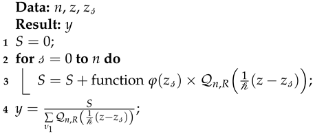
Next, we give several illustrative examples with the help of Matlab algorithms to verify the convergence behavior, computational efficiency, and consistency of the interpolation neural network operators activated by the ramp function ${\varsigma }_R\left(\mathcal{z}\right)$. The possible effects of the ramp function on the absolute error of approximation of the operators ${\mathcal{F}}_{\mathcal{n}}\left(\phi \right)$ are examined in the following tables and graphs in one case. Also, through Algorithm 1, we will give the implementation steps.

Algorithm 1: Implementing the interpolation NN operators (4) activated by smooth ramp functions.

Example 1. 

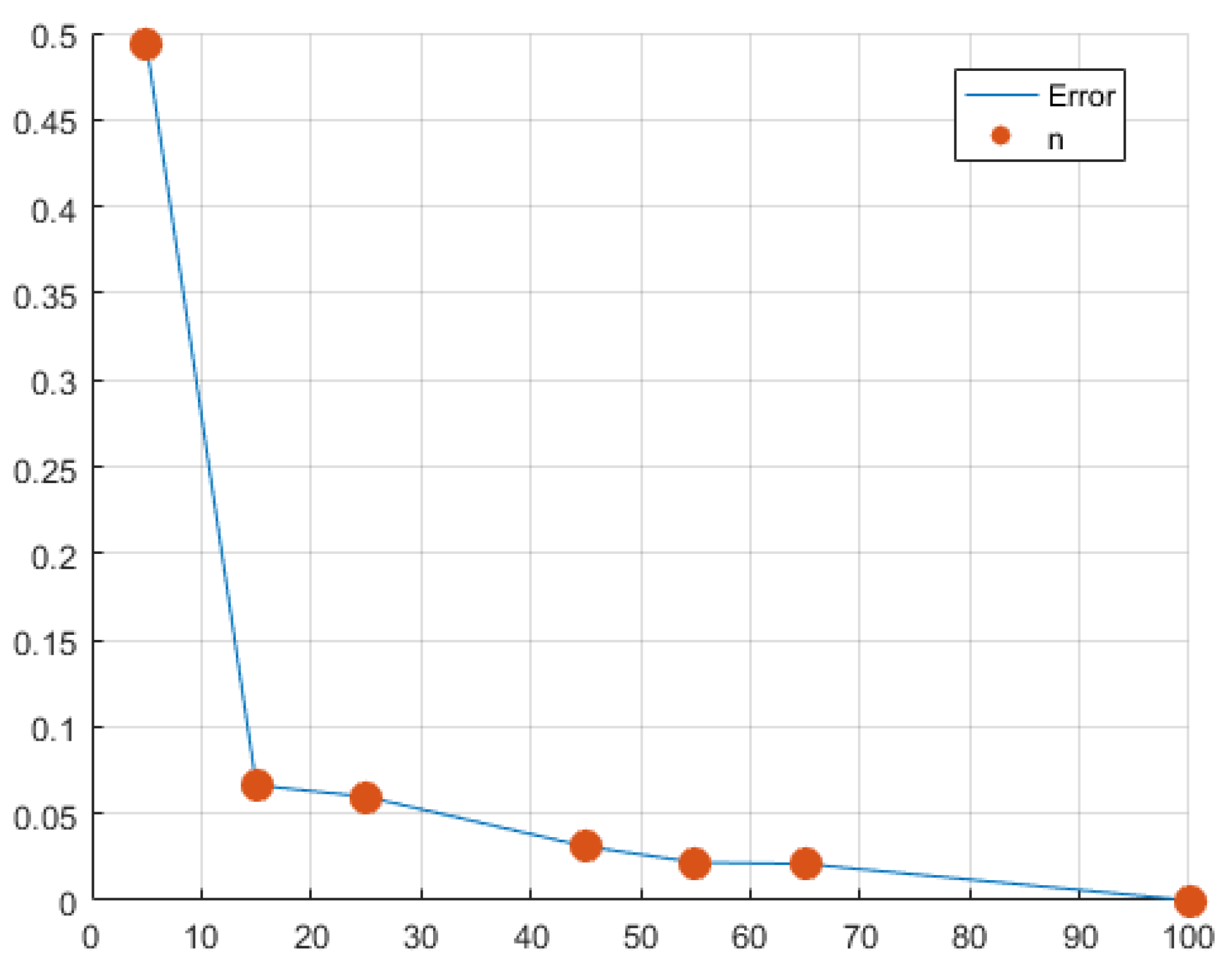
Let us take the operators defined in the relation (4). We now apply the interpolation neural network operators activated by ramp function ${\varsigma }_R\left(\mathcal{z}\right)$ to the function $\psi \left(\mathcal{z}\right)=6e^{-3{\mathcal{z}}^2}sin(2\pi \mathcal{z}/3)$ with $\mathcal{n}=5,15,25,45,55,65$, and $100.$ Let ${\mathcal{E}}_{\mathcal{n}}(\phi ;\mathcal{z})=|{\mathcal{F}}_{\mathcal{n}}\left(\phi \right)\left(\mathcal{z}\right)-\phi \left(\mathcal{z}\right)|,$ the error function of approximation by ${\mathcal{F}}_{\mathcal{n}}\left(\phi \right)$ operators. Figure 1a demonstrates that the operators ${\mathcal{F}}_{\mathcal{n}}\left(\phi \right)$ have a good approximation performance in the one-dimensional case while the error in the approximation is shown in Figure 1b. In

Table 1. Error of approximation ${\mathcal{E}}_{\mathcal{n}}$ for $\mathcal{n}$ = 5, 15, 25, 45, 55, 65, and 100.

$\mathcal{z}$	${\mathcal{E}}_5$	${\mathcal{E}}_{15}$	${\mathcal{E}}_{25}$	${\mathcal{E}}_{45}$	${\mathcal{E}}_{55}$	${\mathcal{E}}_{65}$	${\mathcal{E}}_{100}$
−1	0	0	0	0	0	0	0
−0.8	0.2235	0.0283	0.0103	0.0032	0.0021	0.0015	0
−0.7	0.392	0.1005	0.0669	0.0364	0.0285	0.025	0
−0.5	0.4932	0.0663	0.0597	0.0311	0.0219	0.021	0
−0.4	0.7079	0.0833	0.0301	0.0093	0.0062	0.0045	4.44$·{10}^{-16}$
−0.1	0.5057	0.2479	0.1222	0.0701	0.0617	0.0491	0
0.1	0.5057	0.2479	0.1222	0.0701	0.0617	0.0491	0
0.4	0.7079	0.0833	0.0301	0.0093	0.0062	0.0045	0
0.5	0.4932	0.0663	0.0597	0.0311	0.0219	0.021	0
0.7	0.392	0.1005	0.0669	0.0364	0.0285	0.025	1.55$·{10}^{-15}$
0.8	0.2235	0.0283	0.0103	0.0032	0.0021	0.0015	0
1	0	0	0	0	0	0	0

, we have computed the error at certain points in $[-1,1]$. We observe that, as the value of $\mathcal{n}$ increases, the approximation becomes better, i.e., for the largest value of $\mathcal{n}$, the error is minimal. In Figure 2 we give correlation between $\mathcal{n}$ = 5, 15, 25, 45, 65, 100, and error in point 0.5.

If we take test points uniformly, the results are shown in

Table 2. Error of approximation ${\mathcal{E}}_{\mathcal{n}}$ for $\mathcal{n}$ = 5, 15, 25, 45, 55, 65, and 100.

$\mathcal{z}$	${\mathcal{E}}_5$	${\mathcal{E}}_{15}$	${\mathcal{E}}_{25}$	${\mathcal{E}}_{45}$	${\mathcal{E}}_{55}$	${\mathcal{E}}_{65}$	${\mathcal{E}}_{100}$
−0.8	0.2235	0.0283	0.0103	0.0032	0.0021	0.0015	0
−0.4	0.7079	0.0833	0.0301	0.0093	0.0062	0.0045	4.44$·{10}^{-16}$
0	1.55$·{10}^{-15}$	0	0	0	0	0	0
0.4	0.7079	0.0833	0.0301	0.0093	0.0062	0.0045	0
0.8	0.2235	0.0283	0.0103	0.0032	0.0021	0.0015	0

.

Example 2. 

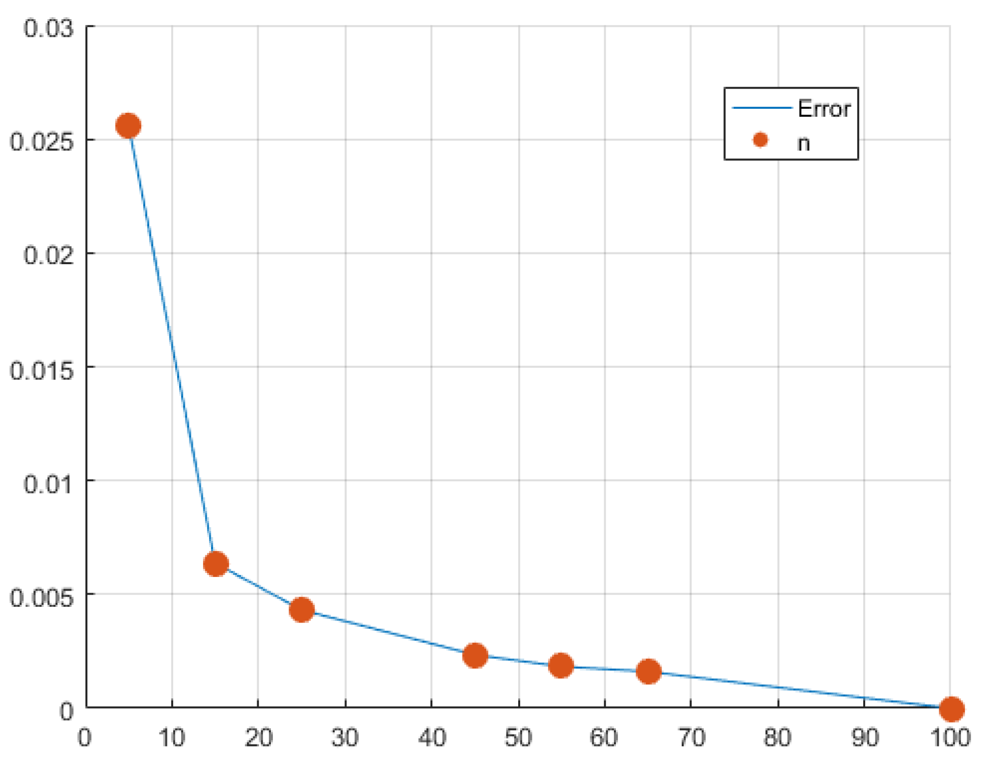
We now apply the interpolation neural network operators activated by the ramp function ${\varsigma }_R\left(\mathcal{z}\right)$ to the function $\psi \left(\mathcal{z}\right)={\mathcal{z}}^{2}sin(1/(\mathcal{z}+1)$ with $\mathcal{n}=5,15,25,45,55,65$, and $100.$ Figure 3a demonstrates that the operators ${\mathcal{F}}_{\mathcal{n}}\left(\phi \right)$ have a good approximation performance in the one-dimensional case while the error in the approximation is shown in Figure 3b. In

Table 3. Error of approximation ${\mathcal{E}}_{\mathcal{n}}$ for $\mathcal{n}$ = 5, 15, 25, 45, 55, 65, and 100.

$\mathcal{z}$	${\mathcal{E}}_5$	${\mathcal{E}}_{15}$	${\mathcal{E}}_{25}$	${\mathcal{E}}_{45}$	${\mathcal{E}}_{55}$	${\mathcal{E}}_{65}$	${\mathcal{E}}_{100}$
−0.9	0.1397	0.0319	0.0228	0.0123	0.0095	0.0085	0
−0.7	0.0423	0.0259	0.0128	0.0074	0.0065	0.0052	0
−0.4	0.0348	0.0038	0.0014	4.26$·{10}^{-4}$	2.85$·{10}^{-4}$	2.04$·{10}^{-4}$	5.55$·{10}^{-17}$
−0.1	0.5057	0.2479	0.1222	0.0701	0.0617	0.0491	0
0.3	0.0082	0.0053	0.0025	0.0015	0.0013	0.001	0
0.5	0.0256	0.0064	0.0043	0.0024	0.0018	0.0016	0
0.9	0.0335	0.0098	0.0062	0.0034	0.0027	0.0024	0

, we have computed the error at certain points in $[-1,1]$. We observe that, as the value of $\mathcal{n}$ increases, the approximation becomes better, i.e., for the largest value of $\mathcal{n}$, the error is minimal. The computational efficiency lies in the fact that, with the increase of $\mathcal{n}$, the error very quickly reaches a value close to zero. In Figure 4 we give correlation between $\mathcal{n}$ = 5, 15, 25, 45, 65, 100, and error in point 0.5.

If we take test points uniformly, the results are shown in

Table 4. Error of approximation ${\mathcal{E}}_{\mathcal{n}}$ for $\mathcal{n}$ = 5, 15, 25, 45, 55, 65, and 100.

$\mathcal{z}$	${\mathcal{E}}_5$	${\mathcal{E}}_{15}$	${\mathcal{E}}_{25}$	${\mathcal{E}}_{45}$	${\mathcal{E}}_{55}$	${\mathcal{E}}_{65}$	${\mathcal{E}}_{100}$
−0.8	0.0649	0.0072	0.0026	8.01$·{10}^{-4}$	5.36$·{10}^{-4}$	3.84$·{10}^{-4}$	0
−0.4	0.0348	0.0038	0.0014	4.26$·{10}^{-4}$	2.85$·{10}^{-4}$	2.04$·{10}^{-4}$	5.55$·{10}^{-17}$
0	0.0193	0.0021	7.67$·{10}^{-4}$	2.37$·{10}^{-4}$	1.59$·{10}^{-4}$	1.13E-04	0
0.4	0.0116	0.0013	4.60$·{10}^{-4}$	1.42$·{10}^{-4}$	9.50$·{10}^{-5}$	6.80$·{10}^{-5}$	0
0.8	0.0074	8.18$·{10}^{-4}$	2.94$·{10}^{-4}$	9.08$·{10}^{-5}$	6.08$·{10}^{-5}$	4.35$·{10}^{-5}$	0

.

5. Conclusive Remarks

In this paper, we studied the approximation properties of a novel family of interpolation NN operators based on the ramp function. The construction and approximation results for the family of operators ${\mathcal{F}}_{\mathcal{n}}\left(\phi \right)\left(\mathcal{z}\right)$ in order to improve the approximation rate to smooth functions have been discussed. We have extended our study to the iterated and complex cases of the operators ${\mathcal{F}}_{\mathcal{n}}\left(\phi \right)\left(\mathcal{z}\right).$ It is interesting to mention that, in the approximation process by our proposed family of operators, one can consider the known sample values in ${\mathcal{F}}_{\mathcal{n}}\left(\phi \right)\left(\mathcal{z}\right)$ as a training data for the network. The convergence results for the proposed operators in this article demonstrate its ability to depict the values extending beyond the confines of the training set. Finally, we gave several illustrative examples with the help of Matlab algorithms to verify the convergence behavior, computational efficiency, and consistency of the neural network operators activated by smooth ramp functions.

References

1. Costarelli, D.; Vinti, G. Approximation by nonlinear multivariate sampling-Kantorovich type operators and applications to image processing. Numer. Funct. Anal. Optim. 2013, 34, 819–844. [Google Scholar] [CrossRef]
2. Cybenko, G. Approximation by superpositions of sigmoidal function. Math. Control Signals Syst. 1989, 2, 303–314. [Google Scholar] [CrossRef]
3. Barron, A.R. Universal approximation bounds for superpositions of a sigmodal function. IEEE Trans. Inform. 1993, 39, 930–945. [Google Scholar] [CrossRef]
4. Costarelli, D.; Spigler, R. Convergence of a family of neural network operators of the Kantorovich type. J. Approx. Theory 2014, 185, 80–90. [Google Scholar] [CrossRef]
5. Anastassiou, G.A. Rate of Convergence of Some Neural Network Operators to the Unit-Univariate Case. J. Math. Anal. Appl. 1997, 212, 237–262. [Google Scholar] [CrossRef]
6. Anastassiou, G.A. Univariate hyperbolic tangent neural network approximation. Math. Comput. Model. 2011, 53, 1111–1132. [Google Scholar] [CrossRef]
7. Anastassiou, G.A. Multivariate hyperbolic tangent neural network approximation. Comput. Math. Appl. 2011, 61, 809–821. [Google Scholar] [CrossRef]
8. Cardaliaguet, P.; Euvrard, G. Approximation of a function and its derivative with a neural network. Neural Netw. 1992, 5, 207–220. [Google Scholar] [CrossRef]
9. Costarelli, D.; Spigler, R. Approximation results for neural network operators activated by sigmoidal functions. Neural Netw. 2013, 44, 101–106. [Google Scholar] [CrossRef]
10. Yu, D.S. Approximation by neural networks with sigmoidal functions. Acta Math. Sin. 2013, 29, 2013–2026. [Google Scholar] [CrossRef]
11. Yu, D.S.; Zhou, P. Approximation by neural network operators activated by smooth ramp functions. Acta Math. Sin. (Chin. Ed.) 2016, 59, 623–638. [Google Scholar]
12. Costarelli, D.; Spigler, R.; Vinti, G. A survey on approximation by means of neural network operators. J. NeuroTechnol. 2016, 1, 29–52. [Google Scholar]
13. Costarelli, D.; Vinti, G. Rate of approximation for multivariate sampling Kantorovich operators on some function spaces. J. Int. Equ. Appl. 2014, 26, 455–481. [Google Scholar] [CrossRef]
14. Costarelli, D.; Vinti, G. Quantitative estimates involving K-functionals for neural network-type operators. Appl. Anal. 2019, 98, 2639–2647. [Google Scholar] [CrossRef]
15. Uyan, H.; Aslan, O.A.; Karateke, S.; Büyükyazıcı, Í. Interpolation for neural network operators activated with a generalized logistic-type function. Preprint 2024. [Google Scholar] [CrossRef]
16. Costarelli, D.; Vinti, G. Voronovskaja type theorems and high-order convergence neural network operators with sigmoidal functions. Mediterr. J. Math. 2020, 17, 23. [Google Scholar] [CrossRef]
17. Coroianu, L.; Costarelli, D.; Kadak, U. Quantitative estimates for neural network operators implied by the asymptotic behaviour of the sigmoidal activation functions. Mediterr. J. Math. 2022, 19, 211. [Google Scholar] [CrossRef]
18. Kadak, U. Multivariate neural network interpolation operators. J. Comput. Appl. Math. 2022, 414, 114426. [Google Scholar] [CrossRef]
19. Qian, Y.Y.; Yu, D.S. Rates of approximation by neural network interpolation operators. Appl. Math. Comput. 2022, 418, 126781. [Google Scholar] [CrossRef]
20. Costarelli, D.; Vinti, G. Approximation by max-product neural network operators of Kantorovich type. Results Math. 2016, 69, 505–519. [Google Scholar] [CrossRef]
21. Costarelli, D.; Vinti, G. Max-product neural network and quasi-interpolation operators activated by sigmoidal functions. J. Approx. Theory 2016, 209, 1–22. [Google Scholar] [CrossRef]
22. Wang, G.S.; Yu, D.S.; Guan, L.M. Neural network interpolation operators of multivariate function. J. Comput. Appl. Math. 2023, 431, 115266. [Google Scholar] [CrossRef]
23. Qian, Y.Y.; Yu, D.S. Neural network interpolation operators activated by smooth ramp functions. Anal. Appl. 2022, 20, 791–813. [Google Scholar] [CrossRef]
24. Wang, G.; Yu, D.; Zhou, P. Neural network interpolation operators optimized by Lagrange polynomial. Neural Netw. 2022, 153, 179–191. [Google Scholar] [CrossRef] [PubMed]
25. Bajpeyi, S.; Kumar, A.S. Approximation by exponential type neural network operators. Anal. Math. Phys. 2021, 11, 108. [Google Scholar] [CrossRef]
26. Bajpeyi, S. Order of approximation for exponential type neural network operators. Results Math. 2023, 78, 99. [Google Scholar] [CrossRef]
27. Mahmudov, N.; Kara, M. Approximation properties of the Reimann–Liouville fractional integral type Szász–Mirakyan–Kantorovich operators. J. Math. Inequal. 2022, 16, 1285–1308. [Google Scholar] [CrossRef]
28. Kadak, U. Fractional type multivariate neural network operators. Math. Methods Appl. Sci. 2023, 46, 3045–3065. [Google Scholar] [CrossRef]
29. Li, F.J. Constructive function approximation by neural networks with optimized activation functions and fixed weights. Neural Comput. Appl. 2019, 31, 4613–4628. [Google Scholar] [CrossRef]
30. Anastassiou, G.A. Fractional Korovkin theory. Chaos Solit. Fract. 2009, 42, 2080–2094. [Google Scholar] [CrossRef]
31. Anastassiou, G. On right fractional calculus. Chaos Solit. Fract. 2009, 42, 365–376. [Google Scholar] [CrossRef]
32. Diethelm, K. The Analysis of Fractional Differential Equations, Lecture Notes in Mathematics 2004; Springer: Berlin/Heidelberg, Germany, 2010. [Google Scholar]
Figure 1. As we increase the value of n , the approximation is good, i.e., for the largest value of n , the error is minimal.
Computation 12 00136 g001
Figure 2. Correlation between n = 5, 15, 25, 45, 65, 100, and error in point 0.5.
Computation 12 00136 g002
Figure 3. As we increase the value of n , the approximation is good, i.e., for the largest value of n , the error is minimal.
Computation 12 00136 g003
Figure 4. Correlation between n = 5, 15, 25, 45, 65, 100 and, error in point 0.5.
Computation 12 00136 g004