Abstract
This work continues the study of the process of friction between a steel spherical indenter and a soft elastic elastomer previously published in our paper. It is done in the context of our previous experimental results obtained on systems with strongly pronounced adhesive interaction between the surfaces of contacting bodies during the process of friction between a steel spherical indenter and a soft elastic elastomer. In the present paper, we concentrate on the theoretical study of the processes developing in a vertical cross-section of the system. For continuity, here the case of indenter motion at a low speed at different indentation depths is considered as before. The analysis of the evolution of normal and tangential contact forces, mean normal pressure, tangential stresses, as well as the size of the contact area is performed. Despite its relative simplicity, a numerical two-dimensional (2D = 1 + 1) model, which is used here, satisfactorily reproduces experimentally observed effects. Furthermore, it allows direct visualization of the motion in the vertical cross-section of the system, which is currently invisible experimentally. Partially, it recalls two-dimensional (2D = 1 + 1) models recently proposed to describe the “turbulent” shear flow of solids under torsion and in cellular materials. The observations extracted from the model help us to understand better the adhesive processes that underlie the experimental results.
1. Introduction
The study of adhesive contacts is one of the actively developing fields of contact mechanics. In normal contact, adhesion can significantly increase the pull-off strength, and in tangential contact, the presence of adhesive interaction can lead to additional energy dissipation. As a result, it can increase friction. Constantly growing interest in the study of adhesion processes is caused by the relationship between the following two factors. First of all, adhesion effects are common in the formation, restructuring and destruction of the contact. Often, they are even easily seen by the naked eye, and their experimental study does not require any expensive equipment. On the other hand, these seemingly simple processes are actually quite complex, requiring the creation of corresponding theories that adequately describe them.
Furthermore, the adhesive technologies have found extensive use in wide range of practically important application areas, for example, in robotics [1,2,3] and medicine [4,5]. The adhesive properties of contacting surfaces play a decisive role in such common technological processes as painting [6,7], soldering [8,9], welding [10,11], gluing surfaces [12,13], coatings [14], etc. The surface roughness partially prevents the creation of good contact [15,16], and as a result, adhesion often does not manifest itself. However, adhesion should be taken into account when developing certain types of microelectronic devices, where the size of contacting objects is small, and adhesive forces between them are significant [17,18]. This is especially critical, for example, for MEMS (micro electric mechanical systems), where contacting surfaces can spontaneously stick to each other due to adhesion [19,20].
The first rigorous theory of adhesive contact was published more than 50 years ago, in 1971. It is the JKR theory [21], which is based on the principle of energy balance and describes the normal adhesive contact between a spherical body and an elastic half-space. In JKR, the radius of action of adhesive forces is assumed to be small compared to other geometric parameters of the problem, such as indentation depth and contact radius. The opposite case of long-range adhesive forces is described by the DMT theory [22], which was published a few years after JKR. Both theories give significantly different results, and only in 1992 in [23] was it shown that they are both limiting cases of the general theory of adhesion, in which the radius of adhesion interaction was introduced as a free parameter.
However, in real experiments, additional effects are almost always observed, that cannot be described using classical theories. For example, there is secondary adhesion hysteresis, which refers to the fact that the loading and unloading phases of the contact formation correspond to different dependences of the normal force on the indentation depth [24,25]. Such hysteresis leads to the additional dissipation of mechanical energy in oscillating adhesive contacts. It must be taken into account in the design of the devices and technological processes wherein adhesion plays an important role. Tangential adhesive contacts, compared to normal ones, show even more complex processes. One can mention, for example, the propagation of elastic waves in the contact zone with simultaneous restructuring of its boundary (Schallamach waves [26,27,28]), changes in the geometric shape of the contact and its area [29,30,31], etc.
Schallamach waves are one of the intriguing phenomena of modern contact mechanics. As a rule, they are observed during the restructuring of contact between soft materials with large elastic deformations (so-called “elastomers”). Elastic gels, which were created recently, are good materials to use to study Schallamach waves. They are optically transparent, have high viscosity and adhesion as well as being able to withstand large elastic deformations. For example, in works [32,33], the sliding of gel samples on a silicate glass surface is studied. They demonstrate a transition between different types of stick–slip motion, which have been studied at different velocities of gel samples driven along the glass. At high speeds, the stick–slip mode is periodic. While velocity decreases, motion becomes irregular and even demonstrates stochastic behavior. Here, chaotic behavior is caused by the fact that at any given moment, the contact between the elastomer and the glass exists in multiple areas, and this complex contact configuration is constantly rearranged during motion. Systems wherein full contact occurs between rubbing surfaces in the stick phase typically exhibit a regular periodic stick–slip motion regime [34,35]. Since the gel material used in [32,33] is transparent, it is possible not only to observe directly the dynamic processes in the contact zone, but also quantitatively determine the corresponding contact area. In turn, one can calculate the value of shear stresses, on which the nature of the propagating elastic waves in the contact zone depends.
In our previous work [36], we experimentally investigated the tangential adhesive contact between a hard steel spherical indenter and a much softer elastomer, at different indentation depths. As an elastomer, the soft gel sheet (thermoplastic polystyrene-type gel sheet, CRG N3005, TANAC Co., Ltd., Gifu, Japan) with thickness h = 25 mm and linear horizontal dimensions 100 mm × 100 mm was used. Note that the much softer CRG N0505 material, produced by the same company, was used in the work cited above [32]. The work [36] considered a quasi-static mode in which the indenter shifted at a very low speed, which was only 1 μm/s. It was shown that, regardless of the indentation depth, in a stationary sliding mode, a regime is established in which constant tangential stresses are distributed throughout the entire contact area, which is a characteristic of the contact, and does not depend on external pressure. In this regime, the friction coefficient becomes meaningless, since the friction force Fx is proportional to the contact area Fx = τ0A, where the stress τ0 is kept constant for all the indentation depths and contact areas.
The constant shear stress τ0 during sliding is often observed in adhesive contacts, and there are two reasons for it. The first reason is that the process of the destruction of adhesive bonds during tangential movement is weakly influenced by external pressure. And the second reason is that in the case wherein one of the contact bodies is sufficiently soft, it is easily deformed and well fills the roughness existing on the surface of the indenter [37]. In this case, the observed (nominal) contact area A is always close to the real one. These two reasons lead to constant shear stresses in contacts in which macroscopic adhesion is observed. In addition to the experiment, ref. [36] proposed a dynamic model of adhesive contact, which confirms the experimental results.
Let us mention, however, one important feature of the work [36] and, in general, of all the experimental works related to the study of quasi-static tangential contact. Despite the fact that in [36], the indenter was moved with a low speed, at the moment when shear stress reached a critical value, partial sliding of rubber developed over the whole surface of the indenter. It ran at a speed many times higher than the shear rate of the indenter by itself and led to the appearance of elastic waves at the interface. This type of systemic excitation causes a propagation of the elastic waves running not only in the interface (which are observed visually), but also inside the bulk of the elastomer material. At the same time, it is quite difficult to experimentally detect these waves without violating the integrity of the system. The creation of dynamic models should help us understand the processes that develop inside the bulk of an adhesive material in this specific friction mode. Let us stress that numerical models are widely applied now as powerful instruments for the visualization of processes in the adhesion contact cross-section. As examples of the frequently used techniques, one can mention the finite element method (FEM) [38,39], molecular dynamics (MD) [40,41] and the method of the movable digital automata [42,43,44,45]. Further, plural analytical models [21,22,23,29,30,31,46,47] are often applied to investigate the adhesion phenomena.
In the present paper, based on the method of interacting movable automata, a model is proposed, with the help of which the modeling of an elastic medium can be naturally performed. Since the purpose of the work is mainly a qualitative description of the processes, a relatively simple and less time-consuming two-dimensional version of the model is considered. The dynamics of this system is quite clear, and one can treat it as a visualization of a two-dimensional cross-section of the adhesive elastomer. The present study continues and compliments the experimental study [36] by a dynamic picture of the propagation of the elastic waves inside an elastomer, in the orthogonal projection, where direct observation in real experiment is a difficult task due to various technological reasons. One has to note that there are fresh works that have experimentally observed the processes in the orthogonal cross-section of the adhesive contact (see, for example, [48]). Their observations look closely at the numerical results that we obtained in the model that is described below.
2. Experimental Technique
The elastic modulus of the elastomer used in experiments in [36] was E ≈ 0.324 MPa, and its Poisson’s ratio was ν ≈ 0.48. The elastomer is several orders of magnitude softer than the other materials used: the substrate (silicon glass) and indenter (steel). So, in the experiment, only the elastomer layer could deform. The elastomeric sample consisted of 5 sheets superimposed on each other; every layer of h = 5 mm thick. Due to mutual adhesion, they were firmly attached to each other. As a result, the elastomer could be practically considered as a solid one with thickness h = 25 mm. In the horizontal direction, the elastomer size was 100 mm × 100 mm.
The radius of the steel indenter, which was pressed into the elastomer, was R = 22 mm. To avoid misunderstandings, let us note that the illustrative photograph in Figure 1 shows only one such elastomer sheet, having the thickness h = 5 mm. The indenter, with a larger radius R than in experiments in [36], is also shown in Figure 1.
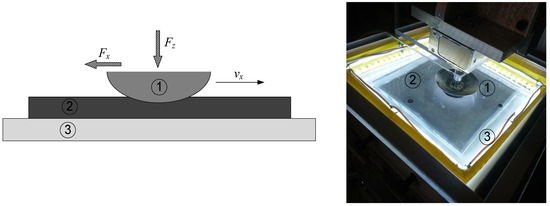
Figure 1.
(Left panel) Simplified experimental design; (right panel) real photograph of the contact zone from [36]: ① indenter, ② elastomeric sample, ③ rigid silicate glass substrate.
3. Numerical Model
Below, to simulate the dynamic behavior of the system under consideration, we apply a combination of numerically generated elastic substrate and movable hard ball with appropriately defined repulsive and adhesion interactions between them. Different possibilities to construct an elastic substrate were described in our previous works (see for example [36,43,44,45]). In particular, one can keep a fixed distance between the particles in the nodes of the mesh of any nature with 4th order potential with two minimums, . Close results can be achieved if one uses quadratic 2-valley potential, . It can be treated, in fact, as a mathematical procedure wherein every node is attracted according to Hook’s law to a local minimum formed by its neighbors in the distances to each of them.
Another possibility was used in the studies [43,44,45], where a lattice was naturally formed by a set of the interacting movable automata supplied by a combination of the short-range repulsion and long-range attraction between the automata, which naturally form a lattice having a fixed distance between the neighbors. Such a system can reproduce a behavior of any viscous “lubricant” placed between two rigid contact surfaces of different forms (planar, spherical, etc.) moving in 3D space. The main features of the system, which have to be reproduced in the model frames, should include an external pressure (including gravitation) acting on at least one of the surfaces. Below, we will call a surface under pressure the “upper” one and describe a shear force caused by the mutual motion of the surfaces.
Let us note that here and below, all the values used in the numerical experiment are normalized to the corresponding measured ones. In particular, a series of experiments, previously published in [36], was carried out with varied indentation depths Dind = 0.0, 0.2, 0.4, 0.6, 0.8 and 1 mm. Normal forces FN at the end of the indentation phase (before the onset of tangential shear), corresponding to the listed indentation depths, were equal to Fz = −0.027, 0.261, 0.765, 1.44, 2.3 and 3.3 N. The corresponding contact areas were equal to A = 6.1, 17.1, 33.66, 51.71, 70.85 and 88.72 mm2, respectively. These values make it possible to calculate the average pressure acting in the contact at different indentation depths <P> = FN/A = −0.0044, 0.015, 0.023, 0.028, 0.032 and 0.037 kPa.
Let us note, additionally, that negative values of normal force Fz and contact pressure <P> at zero indentation depth Dind = 0.0 mm are caused by the fact that in this case, the contact exists only due to adhesion. The adhesive component of the force tends to “pull” the indenter into the elastomer. As a result, to ensure an indentation depth Dind close to zero, it is necessary to apply a negative normal force Fz, i.e., change the direction of its action (see Figure 1). It is interesting that if we formally calculate the friction coefficient μ = Fx/Fz, then it will turn out negative in this case [36]. This fact will be reflected by the numerical results described below.
In our case, one of these surfaces is a rigid spherical ball and another one is the planar substrate. Certainly, such a combination represents quite a standard tribological situation, which should be characterized by the specific geometrical configuration, adhesion, pressure, tangential velocity and other parameters of the problem. In fact, such a model is not restricted to elastic systems only. It allows for a changeable amount of the “lubricant” moving between the surfaces over time. The lubricant can be either gradually added into the space between the surfaces, or extracted from the system, arbitrarily redistributed between them in the course of the whole process or during some transient period, while a balance between the external pressure and bearing force caused by the “lubricant” particles (automata) will be reached. Such a “lubricant” substance combines the ability of extremely strong elastic deformations, including irreversible plastic ones, and some transverse stiffness that allows it to support the upper surface against external pressure. One more advantage of the approach is the following: to hold the automata confined together in arbitrary form, one does not need artificial boundary conditions in addition to the natural ones. Only physical conditions are needed. For example, to keep the system under external load, one needs a repulsing rigid boundary supporting it. We will exploit this advantage below.
Different materials such as those described above were recently simulated by us in the work [43]. Basically, the model used there describes a system of N particles represented by the vector radius ri, the momentum pi, and the interaction potential corresponding to the following Hamiltonian [49]:
For our goals, it is convenient to represent the interaction potential by a pair of the potentials:
where C and D define the magnitude, while c and d describe the radii of attraction and repulsion, respectively. The minimization condition corresponding to an equilibrium reads as follows:
One of the surfaces is moving along a direction x. In different experiments, it can be any of the boundaries between which the automata “particles” are confined. The only physically important things are the following: the particular direction in which an external pressure is applied and the direction in which (normally, orthogonal to it) some of the plates are moving. In this paper, we always treat an “upper” plate as a movable ball of the radius R.
As we mentioned above, the boundary conditions in the horizontal directions of 3D space are not needed. But, one can apply them in some modifications of the model; typically, on a rectangle with the side lengths of [0, Lx] and [0, Ly]. For example, in the case of shear deformation, it is convenient sometimes to employ periodic boundary conditions, wherein a particle leaving the interval [0, Lx] is returned to it at the opposite side of the system. On the vertical axis, the system is limited by a substrate plate at y = 0 that supports the system against gravitation force and/or the normal load P with a reflecting boundary:
To simulate an elastic system, one has to define the initial positions of the automata on some grid where each node is connected with its neighbors by an elastic force. Elastic force tends to conserve the initial distance between the nodes, so such an interaction can be described by the following potential:
Here, R0 is a correlation radius that describes a distance wherein the elastic interaction of the nodes is essentially large. It leads to a linear elastic force at small deviations and automatically keeps the nodes connected with one another on equilibrium distance a. It provides effective longitudinal and lateral stiffness of the material and returns it to the original form when external force is removed.
As in the previous work [36], we add also an interaction between the ball and segments of the elastic substrate. Each particular interaction should be a combination of the repulsion of an elastic segment from the hard “wall” of the ball’s surface and the short-range (adhesive) attraction to the ball in a close proximity to its surface.
It is convenient to simulate them numerically by the sufficiently sharp, but still continuous, potentials. For definiteness, we actually use strong exponential repulsion:
and short-range attraction in a narrow spherical belt around the surface:
Here, and , respectively, while both characteristic distances are much smaller than the radius Rsphere of the spherical ball: Rrepuls << Rsphere, Radh << Rsphere.
The equations of motion have the following form [49]:
where vi is the velocity of the i-th particle. Interacting automata exchange momentum pi, and, hence, a dissipation channel acting to equilibrate relative velocities of the particles that happen to be within the relatively short mutual distance cv, close to the equilibrium one, needs to be introduced. This can be done by including an additive dissipation force,
acting on every particle from the surrounding ones, with corresponding dissipation constant η. As a result, the equations of motion formally assume the following form:
Let us note that here, one deals with a dissipative system, which consists of large numbers of effective particles. So, it is generally expected to demonstrate complex chaotic behavior, typical for such systems [50,51]. Such a behavior can be a topic for an independent study, but it is not a particular aim of the present work. The equations of motion can be integrated by using Verlet’s method, which conserves the energy of the system at each time step, provided no energy is supplied externally through mechanical work or temperature variation.
However, to simulate the effect of adhesion realistically, one has to complete the equations of motion by a condition that specifies when a segment of the substrate follows the ball, being practically glued to it by the adhesion force. Such a condition counts two important features of the adhesion:
- It attaches a given segment of the substrate to the spherical surface when the distance between them is small enough ;
- It detaches the elastic segment from the ball when its deviation from the ball’s surface exceeds a threshold , corresponding to some critical force at given elastic constant k.
In fact, the description above corresponds to a numerical procedure applied at every stage of the simulation routine. But, it also can be formally written in the analytical from as a product of two formal conditions:
where θ is the Heaviside step-function, defined by the standard relations [52]:
The corresponding numerical procedure either solves a set of the dynamic equations for the particular segment, if these threshold conditions are not satisfied, or shifts this elastic segment together with the contacting ball surface, moving according to its own motion. The adhesion indicators are defined (in the same dimensionless units as above) by the distance equal to the unit, as well as the mutual difference of the velocities between the individual automata and indenter and the critical force caused by their displacements from the equilibrium (original) distances , where is the effective elastic constant in Equation (5).
According to above description of the model, our simulation procedure is organized as follows. First of all, we place the ball on the top upper boundary of the elastic slab and allow the system to relax to a state close to equilibrium. This stage is necessary to exclude the errors related to uncertainty in the original position of the elastic mesh at the present values of the repulsion and adhesive potentials of the ball, repulsion of the elastic continuum from the basal (hard solid boundary in the bottom) and other components of the numerical model.
After this, we apply positive (or negative) external load P. If the load is positive, the elastic substrate obviously deforms under its pressure. It causes an opposite force on the ball, which tends to fix it on some equilibrium indentation depth Dind > 0. The motion of the slowly moving ball is described by the equation of motion:
Here, the variables Y and 1/γ describe the vertical position of the ball’s center and the effective relaxation time for the overdamped motion of ball. The ball monotonously moves while all the vertical components of the force balance one another in a self-consistent equilibrium. The balance of the pressure P and total repulsion force naturally defines equilibrium indentation depth Dind. This equilibrium is automatically established despite the uncertainty in the initial position of the ball, elastic medium and external pressure.
When the depth Dind > 0 is defined, one can start pulling the ball in a horizontal direction. This motion obviously causes some nonzero friction in the horizontal direction.
One has to note that in the presence of adhesion, some nonzero indentation depth is still possible at formally negative values of the external load P < 0. In this case, the behavior of the system is not so obvious and trivial, because the adhesive component of the force pulls the ball down. If this force overpowers the external negative load P, the ball goes down to the elastic substrate. Due to the curvature of the spherical ball, the deeper it dives inside the elastic foundation, the larger is the contact area that is formed and, respectively, stronger adhesion becomes possible. In turn, mutual repulsion between rigid ball and elastic foundation, due to the compressibility of the elastic subsystem, grows as well. As a result, some equilibrium distance from the surface can still be established.
However, if negative “load” P < 0 is stronger than some critical one, it overpowers the attraction caused by the adhesion. In this case, some equilibrium negative depth Dind < 0 can be reached. In this case, the ball “levitates” at some positive distance from the (trial) position of the upper boundary of the elastic subsystem. By changing the value P < 0, one can find out a critical value of the negative “load” Pcrit < 0 starting from which the adhesion cannot balance external pulling at all. In this case, the distance between the indenter and surface increases with time because the short-range adhesion force exponentially decreases simultaneously. Adhesion already cannot prevent the vertical motion of the ball, and it leaves proximity of the surface completely. In other words, the absolute value of |Dind(t)| infinitely increases with time: . It is interesting to note that, despite the levitation, up to this threshold P ≤ |Pcrit|, nonzero friction caused by the adhesion is conserved. It is very small, but it still exists.
Results, which are shown in the next section of the article, were obtained with fixed parameters of the model: “length” of the elastomer Lx = 200; “thickness” of the elastomer Ly = 35; number of automata N = 8000; mass of the automata in Equation (1): m = 0.1; parameters of potentials in Equations (2) and (4): C = 10, c = 1, D = 0.1, d = 10; parameters of potential in Equation (5): Kij ≡ K0 = 1, a = 1, R0 = 10−5; parameters of potentials in Equations (6) and (7): radius of the sphere Rsphere = 30, Rrepuls = 1, , Radh = 0.1, ; in Equation (9): cv = 2; “viscosity” in Equation (10): η = 0.25; “adhesive” parameters in Equation (11): δRcrit = 1, fcrit = 3, k = 3; damping coefficient in Equation (13): γ = 0.1; horizontal velocity of the sphere V = 1.
4. Results and Discussion
To establish the difference between the particular regimes, we have performed a numerical simulation of the system under consideration with a sequence of the physically interesting normal loads, including negative ones: P = −50, −45, −10, −5, 0, 25, 50, 75, 100. The main results of the simulation are accumulated in Figure 2, where the time evolution of the contact area, tangential force, normal force and indentation depth are reproduced in the subplots (a)–(d), respectively.
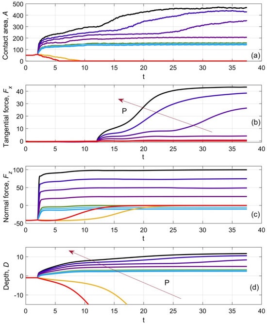
Figure 2.
Time evolution of the contact area A (a), tangential force Fx (b), normal force Fz (c) and indentation depth Dind (d). Saddle point, corresponding to the equilibrium indentation depth close to zero, is shown by the blue line in all the subplots. It is seen from the subplot (a) that it corresponds to a relatively small but nonzero contact area. The yellow and red curves mark the regimes caused by negative pressure smaller than critical Pcrit < 0. Starting from this pressure, the adhesion cannot balance external pulling. It is especially clear from the subplot (d) where red and yellow curves go to infinity. Simultaneously, the contact area falls down to zero after a short transient process. Cian and light blue curves depict the regime wherein the normal force must be negative to support equilibrium indentation P ≤ |Pcrit|. It corresponds to a relatively small but nonzero contact area in asymptotics t→∞ shown in the subplot (a). Ordinary friction regimes that correspond to the monotonously growing positive normal load are depicted by the curves with the colors regularly changing in the fixed color gamma (from magenta to black). Correlation between the particular value of the equilibrium pressure and the color of each curve in the subplots (b,d) is marked by the arrow.
The initial relaxation of the system to the equilibrium continues from t = 0 to t = 2. After this preliminary relaxation, the vertical indentation is performed up to the moment t = 12. After this moment, a tangential shift starts. A corresponding change is clearly seen in the curves drawn in all the subplots, (a)–(d). In addition, one can notice a qualitative change in the behavior in the vicinity of a “saddle point” Pcrit ≈ −10 in the parametric space where the standard friction regime with a relatively deep indentation under a sufficiently strong positive normal load changes into “levitation” or even to detachment regimes. As was expected, the value corresponding to this “saddle point” Pcrit ≈ −10 indentation depth is close to zero. It is depicted by the blue curve in all the subplots of Figure 2.
In particular, the critical regime corresponds to a relatively small but nonzero contact area, as is seen from the subplot (a). The yellow and red curves in the same subplot mark the regimes caused by negative pressure that is smaller than the critical one. As was discussed above, a situation starting from a sufficiently strong negative “load” weakening due to external pulling adhesion cannot balance the negative pressure. This fact is especially clear from the subplot (d), where red and yellow curves, after a short transient process, diverge to infinity. The rate of the divergency definitely depends on the strength of the pulling force. It is different for two presented values of the parameter: P = −50, −45. Simultaneously with the deviation of the ball from the surface, the contact area quickly falls down to zero after a short transient process.
Cian and light blue curves depict the regime wherein, due to the adhesion, the normal force must be negative to support static equilibrium indentation. It corresponds to a relatively small but nonzero asymptotic contact area at t→∞, shown by the curves of the same color in the subplot (a). The family of other curves represents ordinary friction regimes at a monotonously growing normal load. Their colors gradually vary from magenta to black. The correlation between the particular value of the equilibrium pressure and the color of each curve in the subplots (b) and (d) is marked by the arrows. In both cases, when the ball is completely detached from the substrate at the end of the process (red and yellow curves), the asymptotic vertical force monotonously tends toward zero after the moment of detaching.
The fine structure of the instant configuration of the system during tangential motion at intermediate normal load P = 25 is presented in Figure 3.
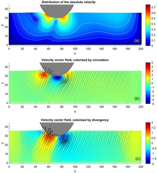
Figure 3.
Typical instant configuration of the system at intermediate normal load P = 25. Subplot (a) reproduces spatial distribution of the absolute local velocities normalized to the pulling velocity , where deep red and blue colors correspond to the large and small values, respectively. It can be seen directly that the elastic substrate is involved in the motion of the ball mainly near a region of the contact. The subplot (b) reproduces the vector field of the local velocity that overlaps the density of its circulation, shown by a colormap. From the comparison with the subplot (a), one can see that two regions of the maximal absolute velocity correspond to the couple of the opposite vortices caused by the ball. The vortex rotates clockwise almost under its bottom, and the anti-vortex rotates counterclockwise behind it. These rotations are accompanied by the waves of the compression and extension shown in the subplot (c) together with the velocity vector field. One can see that the compression mainly takes place in front of the moving ball, while successive extension and compression waves (partially caused by an effect of the adhesion) follow the ball behind it.
Subplot (a) of this figure reproduces the spatial distribution of the absolute local velocities normalized to the tangential pulling velocity . For its visualization, we apply a scatter plot of the movable automata distribution, where deep red and blue colors correspond to the large and small values, respectively.
It can be seen directly from Figure 3a that the elastic substrate is involved in the motion of the ball mainly near a region of the contact. Subplot (b) reproduces the vector field of the same distribution of local velocity as shown in subplot (a), which overlaps the density of its circulation, shown by a colormap. One can establish a relation between the distributions of the absolute velocity and intensity of the circulation from the subplots (a) and (b), respectively. The only mutual relation of the calculated values has a meaning. The distances are measured in the units shown directly on the vertical and horizontal axes of the plots. In these units, the radius of the indenter, used for the particular simulation (also shown by the part of the gray circle) is equal to R = 30. The tangential velocity is equal to the unit as well: Vx = 1. All the densities are reproduced in the standard MatLab colormap "jet" and distributed (in the same dimensionless units). For the movable digital automata, it is done by a so-called “scatter-plot” of MatLab, where every automaton has an individual color corresponding to the desirable value. The continuous densities seen in Figure 3 are a kind of “optical illusion” caused by the large number of automata densely parked in the picture.
In particular, it can be seen that two regions of the maximal absolute velocity in subplot (a) actually correspond to a couple of the opposite vortices, caused by the directed motion of the ball. One of them is a vortex, rotating clockwise almost under the bottom of the ball. The second one is anti-vortex, which rotates counterclockwise behind it. These rotations are accompanied by the waves of compression and extension shown in the subplot (c) together with the velocity vector field.
From Figure 3c, one can see also that the compression mainly takes place in front of the moving ball. In contrast to it, successive extension caused by its weaker compression waves follow the ball behind. Partially, the extension of the elastic substance behind the ball is caused by its compression under it, but partially it appears to be due to the adhesion, which can pull the elastic medium to follow the ball behind, because of its attraction to the ball’s surface.
It is interesting to compare vortex structures caused by the motion of the ball in vertical and horizontal directions, which consequently take place at different stages of the process: during its indentation and pulling. For such a comparison, we have plotted the same snapshots, analogous to those shown in Figure 3, but calculated during a stage of vertical indentation without tangential motion at an extremely strong normal load, P = 100.
The corresponding picture is reproduced in Figure 4. The difference in the symmetry of the velocity distribution in subplot (a), as well as in the circulation structure of its vector field, and the compression presented for this case in subplots (b) and (c), respectively, can be seen directly. One can see in Figure 4b a couple of the symmetrical-appearing vortex and antivortex. They are accompanied by the obvious region of compression that emerged under the ball due to the simultaneous extrusion of the material symmetrically to the left and right sides of the ball. It is useful, also, to compare the vortex structure caused by the motion of the ball in the vertical direction at a positive (as in Figure 4) and “negative” normal load. In the second case, the ball is actually lifted from a trial position, which will be either stopped by the adhesion force, with a relatively weak lifting force, or will continue to move out with infinitely increasing distance.
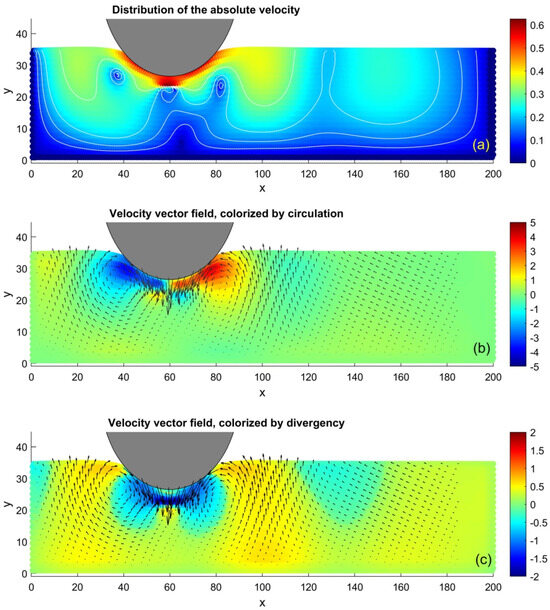
Figure 4.
The same as in Figure 3, calculated in a stage of vertical indentation at large normal load P = 100 for a comparison with the horizontal pulling. The difference in the symmetry of the velocity distribution in the subplot (a), as well as in the circulation structure of its vector field and compression in the subplots (b) and (c), respectively, can be seen directly. One can see here a couple of the symmetric vortex and antivortex accompanied by the obvious compression under the ball leading to the extrusion of the material to its left and right sides.
The typical configuration obtained for the “negative” load P = −40 is reproduced in Figure 5. The difference in the velocity distribution shown in subplot (a) of this figure, as well as in the circulation structure of its vector field and compression in subplots (b) and (c) at positive indentation force P = 100, shown in Figure 4, can be seen directly. In Figure 5b, on each side of the ball, one can see vortex–antivortex pairs. This combination of the vortices is caused here by a combination of the compression of the elastic foundation directly under the ball and its extension on both sides, seen in subplot (c). Respectively, the complexity of these motions leads to more complexity than in the distribution of absolute velocity shown in Figure 4a. In Figure 5a, this distribution has three maximums: under the ball directly and on both of its sides. These maximums are separated by the belts of smaller velocity between them.
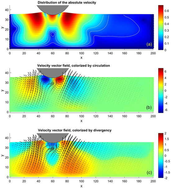
Figure 5.
The same as in Figure 4, calculated in a stage of vertical lifting of the ball with “negative normal load” P = −40. The complexity of deformations leads to a corresponding distribution of the absolute velocity shown in subplot (a). It has a maximum directly under the ball and two maximums on both its sides. They are separated by belts of small absolute velocity. On each side of the ball in subplot (b), one can see a couple of vortex–antivortex pairs, caused here by a combination of compression of the elastic foundation directly under the ball and its extension on both sides. These deformations are seen in subplot (c).
Time evolution of the system in dynamics is reproduced in the Supplementary Materials: Videos S1–S3, where the process in dynamics is presented for different normal loads, respectively:
- (a)
- At positive normal load P = 25;
- (b)
- Strong “negative normal load” P = −40, strong enough to detach the ball from the adhesive surface;
- (c)
- Intermediate “negative load” P = −5 at which, despite the vertically pulling force, the ball and adhesive substrate attract one another and, as result, move along the deformed surface with some nonzero indentation.
The history of the process is recorded in the static form of the time–space maps in Figure 6. In this figure, the top layer’s tangential velocity and the inverse distance from the ball are plotted in subplots (a) and (b), respectively.
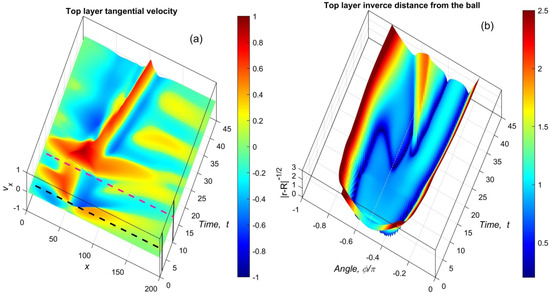
Figure 6.
Time–space distributions of the top layer’s tangential velocity (a) and inverse distance between the ball and top layer (b). The distributions are calculated during a relatively short run after an initial preparation of the system and indentation of the ball. The system is adjusted to the static configuration close to equilibrium during the time interval t1 = 2 and the indentation period after it is up to t2 = 10. They are marked by black and magenta dashed lines, respectively.
These pictures are plotted for a relatively short run of the system to make them clear. As is described above, the system has been preliminary adjusted to the natural static configuration close to equilibrium during the initial time interval, equal to t1 = 2. After this, an indentation with normal load P = 75 during t2 = 10 has been applied. These two time moments are marked by the black and magenta dashed lines in the subplot (a) of the figure, respectively. During this time, as was found in the previous numerical experiments, the system practically stabilizes at the equilibrium indentation. After this, the horizontal motion of the ball is performed with constant velocity. The dimensionless velocity Vx = 1 is shown in all the figures (in fact, all the velocities of the problem are normalized to the pulling one). Both temporal maps in Figure 6a,b are plotted by the surfaces, where large and small values are shown by the deep red and blue colors, respectively.
5. Conclusions
To conclude, in this paper we presented the investigation that continues the study of the process of friction between a steel spherical indenter and a soft elastic elastomer previously published in our paper [36]. It was done in the context of the same experimental studies performed on the systems with strongly pronounced adhesive interactions between a steel spherical indenter and a soft elastic elastomer. In the present paper, we concentrate on the theoretical study of the processes developing in a vertical cross-section of the system. It is shown that despite its relative simplicity, a numerical two–dimensional (2D = 1 + 1) model describes quite well the system under consideration.
The advantage of the model is that it allows visualization of the motion in the vertical cross-section of the system through experimental observation, which became available very recently [48]. It is still very hard to observe this, and information about it is still quite limited. At the same time, the model satisfactorily describes the experimentally observed effects and qualitatively reproduces the correct behavior of the physical system. Numerical experiments in the frame of this model can be used to obtain a better understanding of the adhesive processes, which underlie our physical expectations and are very difficult to observe visually.
Supplementary Materials
The following supporting information can be downloaded at https://www.mdpi.com/article/10.3390/computation12050107/s1, Video S1: Dynamics of the indentation at positive normal load P = 25. Spatial distributions of the absolute local velocities, velocity vector field circulation and local extensions and compressions (divergency) are shown by MatLab colormap “jet” in the corresponding subplots. Three stages: preliminary preparation of the equilibrium system, static indentation and pulling are seen consequently. Video S2: The same as in the first movie, obtained at strong "negative normal load", P = −40. It can be seen that after an initial (preparation) stage, the ball detaches from the surface, being pulled by the external force, and moves further in a vertical direction. Video S3: The same as in the first movie, obtained at a relatively weak “negative normal load”, P = −5. It can be seen that after an initial (preparation) stage, the ball remains touching the surface and moves with some indentation depth corresponding to an equilibrium between adhesion and the vertical component of the pulling force. It can be seen also that despite a “negative load”, a horizontal motion of the ball causes density waves and circulations in a manner qualitatively analogous to that caused by the positive normal load.
Author Contributions
Scientific supervision, project administration, writing—review and editing, V.L.P.; conceptualization, methodology, software, simulation, data analysis, visualization (figures, Supplementary Videos), writing—original draft preparation, A.E.F.; data analysis, writing—original draft preparation, writing—review and editing, I.A.L. All authors have read and agreed to the published version of the manuscript.
Funding
This research was funded by Deutsche Forschungsgemeinschaft (Project DFG PO 810/55-3).
Data Availability Statement
The datasets generated for this study are available upon request from the corresponding author.
Acknowledgments
We acknowledge support by the Open Access Publication Fund of TU Berlin.
Conflicts of Interest
The authors declare no conflicts of interest.
References
- Weston-Dawkes, W.P.; Adibnazari, I.; Hu, Y.-W.; Everman, M.; Gravish, N.; Tolley, M.T. Gas-Lubricated Vibration-Based Adhesion for Robotics. Adv. Intell. Syst. 2021, 3, 2100001. [Google Scholar] [CrossRef]
- Zheng, M.; Wang, D.; Zhu, D.; Cao, S.; Wang, X.; Zhang, M. PiezoClimber: Versatile and Self-Transitional Climbing Soft Robot with Bioinspired Highly Directional Footpads. Adv. Funct. Mater. 2023, 34, 2308384. [Google Scholar] [CrossRef]
- Son, C.; Jeong, S.; Lee, S.; Ferreira, P.M.; Kim, S. Tunable Adhesion of Shape Memory Polymer Dry Adhesive Soft Robotic Gripper via Stiffness Control. Robotics 2023, 12, 59. [Google Scholar] [CrossRef]
- Ge, L.; Chen, S. Recent Advances in Tissue Adhesives for Clinical Medicine. Polymers 2020, 12, 939. [Google Scholar] [CrossRef] [PubMed]
- Mitchell, J.; Lo, K.W.-H. The Use of Small-Molecule Compounds for Cell Adhesion and Migration in Regenerative Medicine. Biomedicines 2023, 11, 2507. [Google Scholar] [CrossRef]
- Suzuki, H.; Ejima, H.; Ohnishi, I.; Ichiki, T.; Shibuta, Y. Molecular Dynamics Simulation of Adhesion of Additive Molecules in Paint Materials toward Enhancement of Anticorrosion Performance. ACS Omega 2024, 9, 4656–4663. [Google Scholar] [CrossRef]
- Peng, X.; Zhang, Z. Improvement of paint adhesion of environmentally friendly paint film on wood surface by plasma treatment. Prog. Org. Coat. 2019, 134, 255–263. [Google Scholar] [CrossRef]
- Fischer-Hirchert, U.H.P. Soldering, Adhesive Bonding, and Bonding. In Photonic Packaging Sourcebook; Springer: Berlin/Heidelberg, Germany, 2015. [Google Scholar] [CrossRef]
- De Rose, A.; Kamp, M.; Mikolasch, G.; Kraft, A.; Nowottnick, M. Adhesion improvement for solder interconnection of wet chemically coated aluminum surfaces. AIP Conf. Proc. 2019, 2156, 020014. [Google Scholar] [CrossRef]
- Antelo, J.; Akhavan-Safar, A.; Carbas, R.J.C.; Marques, E.A.S.; Goyal, R.; da Silva, L.F.M. Replacing welding with adhesive bonding: An industrial case study. Int. J. Adhes. Adhes. 2022, 113, 103064. [Google Scholar] [CrossRef]
- Sancaktar, E. Polymer adhesion by ultrasonic welding. J. Adhes. Sci. Technol. 1999, 13, 179–201. [Google Scholar] [CrossRef]
- Szewczak, A. Influence of Epoxy Glue Modification on the Adhesion of CFRP Tapes to Concrete Surface. Materials 2021, 14, 6339. [Google Scholar] [CrossRef] [PubMed]
- Kreitschitz, A.; Kovalev, A.; Gorb, S.N. Plant Seed Mucilage as a Glue: Adhesive Properties of Hydrated and Dried-in-Contact Seed Mucilage of Five Plant Species. Int. J. Mol. Sci. 2021, 22, 1443. [Google Scholar] [CrossRef] [PubMed]
- Makukha, Z.M.; Protsenko, S.I.; Odnodvorets, L.V.; Protsenko, I.Y. Magneto-strain effect in double-layer film systems. J. Nano-Electron. Phys. 2012, 4, 02043. [Google Scholar]
- Aghababaei, R.; Brodsky, E.E.; Molinari, J.F.; Chandrasekar, S. How roughness emerges on natural and engineered surfaces. MRS Bull. 2022, 47, 1229–1236. [Google Scholar] [CrossRef]
- Pogrebnjak, A.D.; Borisyuk, V.N.; Bagdasaryan, A.A.; Maksakova, O.V.; Smirnova, E.V. The multifractal investigation of surface microgeometry of (Ti-Hf-Zr-V-Nb)N nitride coatings. J. Nano-Electron. Phys. 2014, 6, 04018. [Google Scholar]
- Chernov, S.V.; Makukha, Z.M.; Protsenko, I.Y.; Nepijko, S.A.; Elmers, H.J.; Schönhense, G. Test object for emission electron microscope. Appl. Phys. A 2014, 114, 1383–1385. [Google Scholar] [CrossRef]
- Weinstein, T.; Gilon, H.; Filc, O.; Sammartino, C.; Pinchasik, B.-E. Automated Manipulation of Miniature Objects Underwater Using Air Capillary Bridges: Pick-and-Place, Surface Cleaning, and Underwater Origami. ACS Appl. Mater. Interfaces 2022, 14, 9855–9863. [Google Scholar] [CrossRef]
- Rusu, F.; Pustan, M.; Bîrleanu, C.; Müller, R.; Voicu, R.; Baracu, A. Analysis of the surface effects on adhesion in MEMS structures. Appl. Surf. Sci. 2015, 358 Pt B, 634–640. [Google Scholar] [CrossRef]
- Gkouzou, A.; Kokorian, J.; Janssen, G.C.A.M.; van Spengen, W.M. Controlling adhesion between multi-asperity contacting surfaces in MEMS devices by local heating. J. Micromech. Microeng. 2016, 26, 095020. [Google Scholar] [CrossRef]
- Johnson, K.L.; Kendall, K.; Roberts, A.D. Surface energy and the contact of elastic solids. Proc. R. Soc. Lond. A 1971, 324, 301–313. [Google Scholar] [CrossRef]
- Derjaguin, B.V.; Muller, V.M.; Toporov, Y.P. Effect of contact deformations on the adhesion of particles. J. Colloid Interface Sci. 1975, 53, 314–326. [Google Scholar] [CrossRef]
- Maugis, D. Adhesion of spheres: The JKR-DMT-transition using a Dugdale model. J. Colloid Interface Sci. 1992, 150, 243–269. [Google Scholar] [CrossRef]
- Attard, P. Interaction and Deformation of Elastic Bodies: Origin of Adhesion Hysteresis. J. Phys. Chem. B 2000, 104, 10635–10641. [Google Scholar] [CrossRef]
- Qian, L.; Yu, B. Adhesion Hysteresis. In Encyclopedia of Tribology; Wang, Q.J., Chung, Y.W., Eds.; Springer: Boston, MA, USA, 2013. [Google Scholar] [CrossRef]
- Schallamach, A. How does rubber slide? Wear 1971, 17, 301–312. [Google Scholar] [CrossRef]
- Barquins, M. Sliding Friction of Rubber and Schallamach Waves—A Review. Mater. Sci. Eng. 1985, 73, 45–63. [Google Scholar] [CrossRef]
- Rand, C.J.; Crosby, A.J. Insight into the periodicity of Schallamach waves in soft material friction. Appl. Phys. Lett. 2006, 89, 261907. [Google Scholar] [CrossRef]
- Savkoor, A.R.; Briggs, G.A.D. The effect of tangential force on the contact of elastic solids in adhesion. Proc. R. Soc. Lond. A. Math. Phys. Sci. 1977, 356, 103–114. [Google Scholar]
- Mergel, J.C.; Sahli, R.; Scheibert, J.; Sauer, R.A. Continuum contact models for coupled adhesion and friction. J. Adhes. 2019, 95, 1101–1133. [Google Scholar] [CrossRef]
- Salehani, M.K.; Irani, N.; Nicola, L. Modeling adhesive contacts under mixed-mode loading. J. Mech. Phys. Solids 2019, 130, 320–329. [Google Scholar] [CrossRef]
- Morishita, M.; Kobayashi, M.; Yamaguchi, T.; Doi, M. Observation of spatio-temporal structure in stick-slip motion of an adhesive gel sheet. J. Phys. Condens. Matter 2010, 22, 365104. [Google Scholar] [CrossRef]
- Yamaguchi, T.; Ohmata, S.; Doi, M. Regular to chaotic transition of stick-slip motion in sliding friction of an adhesive gel-sheet. J. Phys. Condens. Matter 2009, 21, 205105. [Google Scholar] [CrossRef]
- Lyashenko, I.A.; Khomenko, A.V.; Zaskoka, A.M. Hysteresis Behavior in the Stick-Slip Mode at the Boundary Friction. Tribol. Trans. 2013, 56, 1019–1026. [Google Scholar] [CrossRef]
- Chen, W.; Foster, A.S.; Alava, M.J.; Laurson, L. Stick-Slip Control in Nanoscale Boundary Lubrication by Surface Wettability. Phys. Rev. Lett. 2015, 114, 095502. [Google Scholar] [CrossRef] [PubMed]
- Lyashenko, I.A.; Filippov, A.E.; Popov, V.L. Friction in Adhesive Contacts: Experiment and Simulation. Machines 2023, 11, 583. [Google Scholar] [CrossRef]
- Ozaki, S.; Mieda, K.; Matsuura, T.; Maegawa, S. Simple Prediction Method for Rubber Adhesive Friction by the Combining Friction Test and FE Analysis. Lubricants 2018, 6, 38. [Google Scholar] [CrossRef]
- Luo, J.; Liu, J.; Xia, H.; Ao, X.; Fu, Z.; Ni, J.; Huang, H. Finite Element Analysis of Adhesive Contact Behaviors in Elastoplastic and Viscoelastic Media. Tribol. Lett. 2024, 72, 7. [Google Scholar] [CrossRef]
- Forsbach, F.; Heß, M.; Papangelo, A. A two-scale FEM-BAM approach for fingerpad friction under electroadhesion. Front. Mech. Eng. 2023, 8, 1074393. [Google Scholar] [CrossRef]
- Baker, A.J.; Vishnubhotla, S.B.; Chen, R.; Martini, A.; Jacobs, T.D.B. Origin of Pressure-Dependent Adhesion in Nanoscale Contacts. Nano Lett. 2022, 22, 5954–5960. [Google Scholar] [CrossRef] [PubMed]
- Tong, R.T.; Zhang, X.; Zhang, T.; Du, J.-T.; Liu, G. Molecular Dynamics Simulation on Friction Properties of Textured Surfaces in Nanoscale Rolling Contacts. J. Mater. Eng. Perform. 2022, 31, 5736–5746. [Google Scholar] [CrossRef]
- Smolin, A.Y.; Eremina, G.M.; Sergeev, V.V.; Shilko, E.V. Three-dimensional movable cellular automata simulation of elastoplastic deformation and fracture of coatings in contact interaction with a rigid indenter. Phys. Mesomech. 2014, 17, 292–303. [Google Scholar] [CrossRef]
- Beygelzimer, Y.; Filippov, A.E.; Estrin, Y. ‘Turbulent’ shear flow of solids under high-pressure torsion. Philos. Mag. 2023, 103, 1017–1028. [Google Scholar] [CrossRef]
- Fillipov, A.E.; Hu, B.; Li, B.; Zeltser, A. Energy transport between two attractors connected by a Fermi–Pasta–Ulam chain. J. Phys. A Math. Gen. 1998, 31, 7719–7728. [Google Scholar] [CrossRef]
- Filippov, A.E.; Klafter, J.; Urbakh, M. Friction through dynamical formation and rupture of molecular bonds. Phys. Rev. Lett. 2004, 92, 135503. [Google Scholar] [CrossRef]
- Lyashenko, I.A.; Liashenko, Z.M. Influence of tangential displacement on the adhesion force between gradient materials. Ukr. J. Phys. 2020, 65, 205–216. [Google Scholar] [CrossRef]
- Khudoynazarov, K. Longitudinal-Radial Vibrations of a Viscoelastic Cylindrical Three-Layer Structure. Facta Univ. Ser. Mech. Eng. 2024. [Google Scholar]
- Glover, J.D.; Yang, X.; Long, R.; Pham, J.T. Creasing in microscale, soft static friction. Nat. Commun. 2023, 14, 2362. [Google Scholar] [CrossRef]
- Landau, L.D.; Lifshitz, E.M. Mechanics, 3rd ed.; Butterworth-Heinemann: Oxford, UK, 1976; Volume 1, ISBN 978-0-7506-2896-9. [Google Scholar]
- Haken, H. Information and Self-Organization: A Macroscopic Approach to Complex Systems, 3rd ed.; Springer: Berlin/Heidelberg, Germany, 2006; ISBN 978-3-540-33021-9. [Google Scholar]
- Liashenko, Z.M.; Lyashenko, I.A. Influence of spatial inhomogeneity on the formation of chaotic modes at the self-organization process. Ukr. J. Phys. 2020, 65, 130–142. [Google Scholar] [CrossRef]
- Berg, E.J. “Unit Function”. Heaviside’s Operational Calculus, as Applied to Engineering and Physics; McGraw-Hill Education: New York, NY, USA, 1936; p. 5. [Google Scholar]
Disclaimer/Publisher’s Note: The statements, opinions and data contained in all publications are solely those of the individual author(s) and contributor(s) and not of MDPI and/or the editor(s). MDPI and/or the editor(s) disclaim responsibility for any injury to people or property resulting from any ideas, methods, instructions or products referred to in the content. |
© 2024 by the authors. Licensee MDPI, Basel, Switzerland. This article is an open access article distributed under the terms and conditions of the Creative Commons Attribution (CC BY) license (https://creativecommons.org/licenses/by/4.0/).