
Systematic Investigation of the Explicit, Dynamically Consistent Methods for Fisher’s Equation


Abstract
1. Introduction
2. The Studied Equation and Its Space Discretization
3. The Tested Methods
3.1. The Applied 12 Convex Combination Scheme for the Diffusion Equation
3.2. The Numerical Treatments of the Nonlinear Term
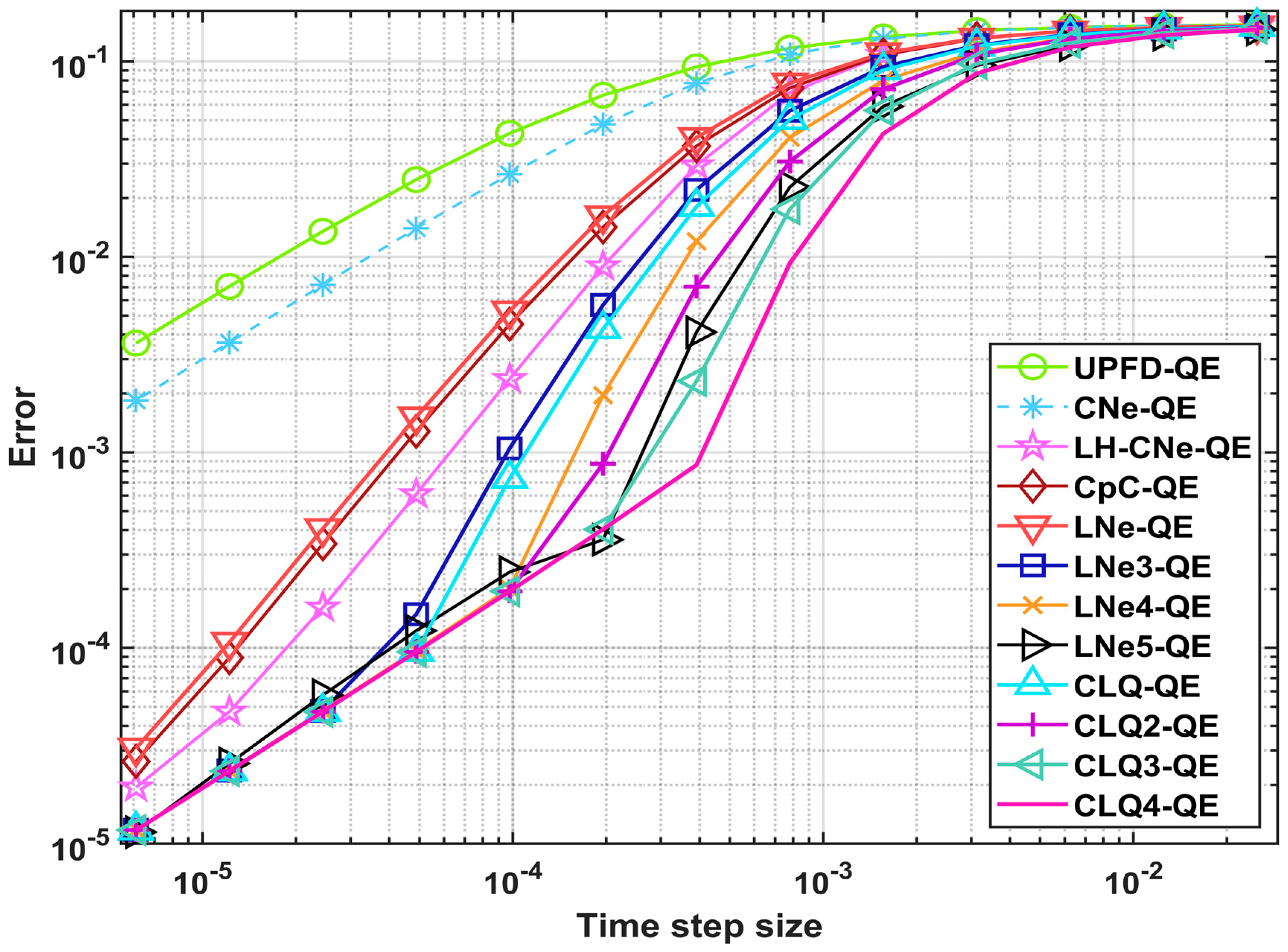
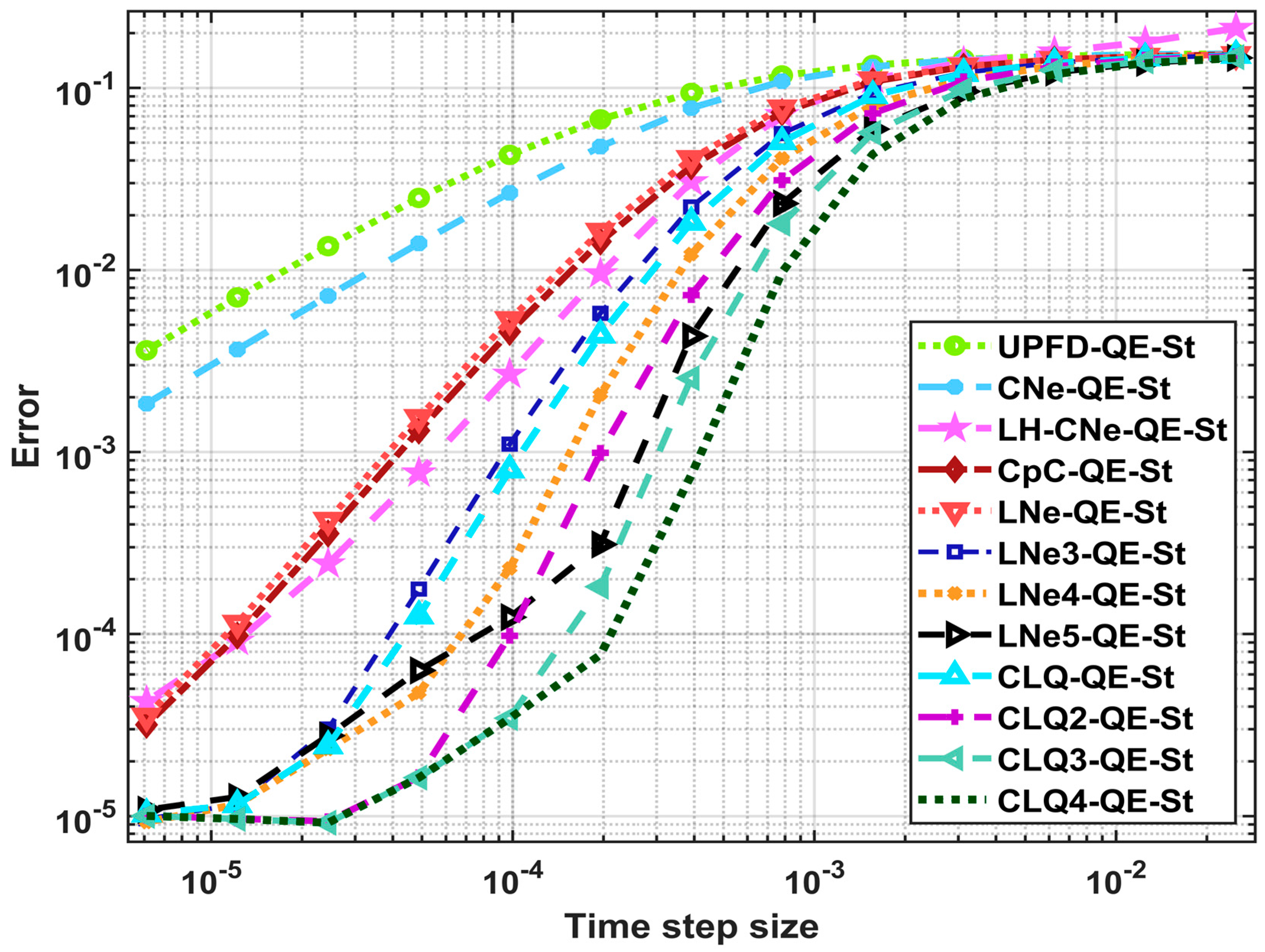
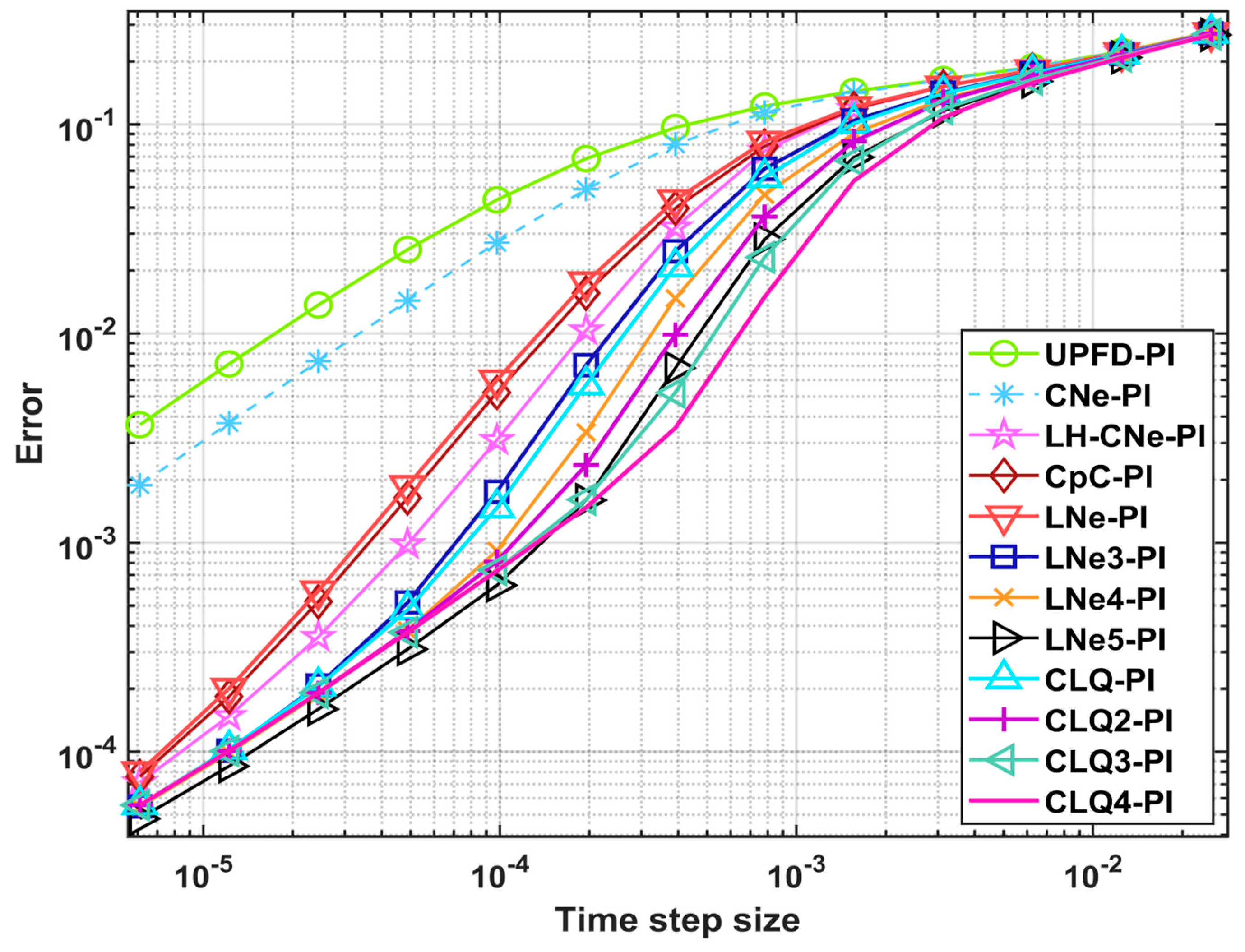
4. Verification in 1D
Experiment 1: One Space Dimension Using an Exact Solution
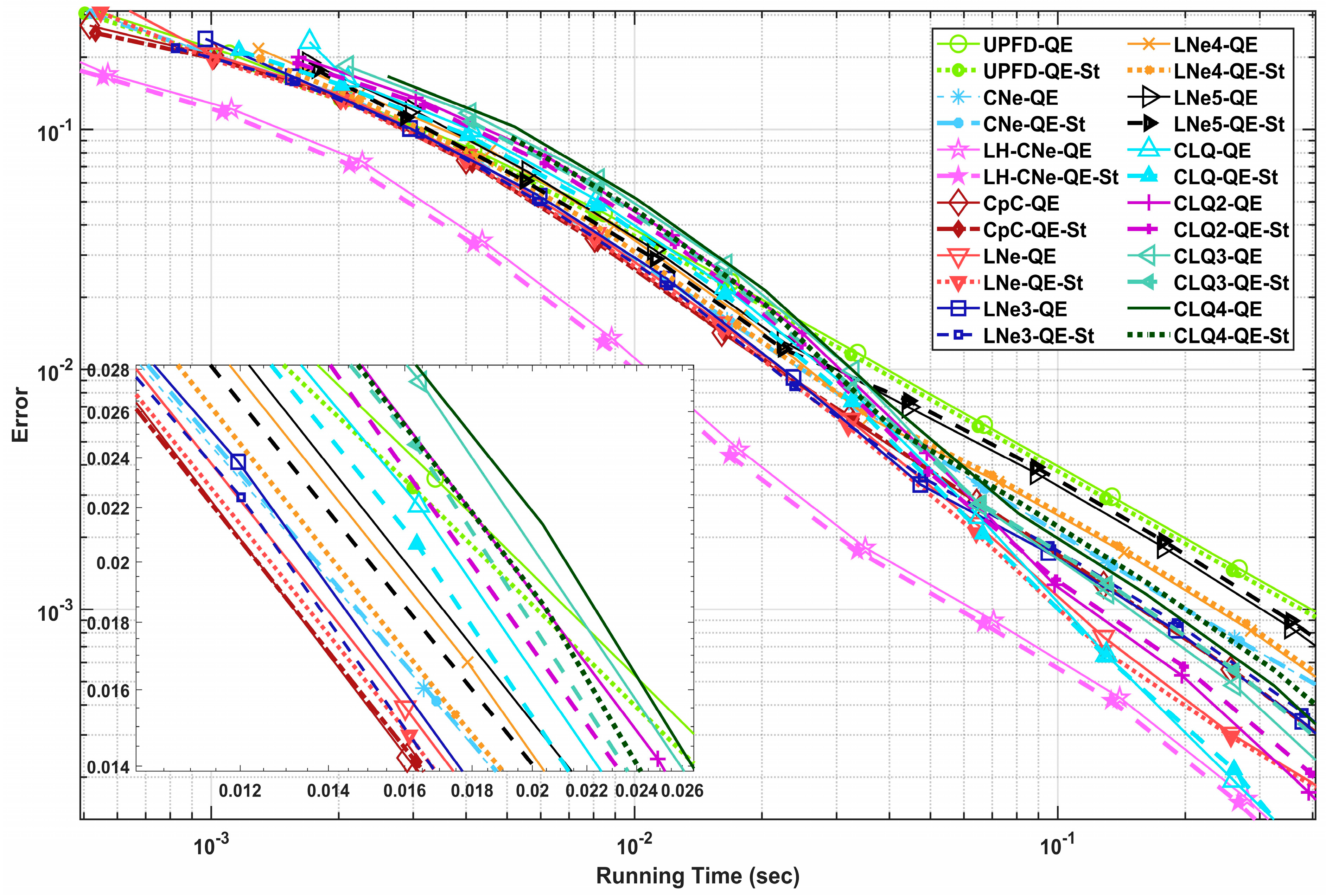
5. Testing of Performance with Running Time Measurements
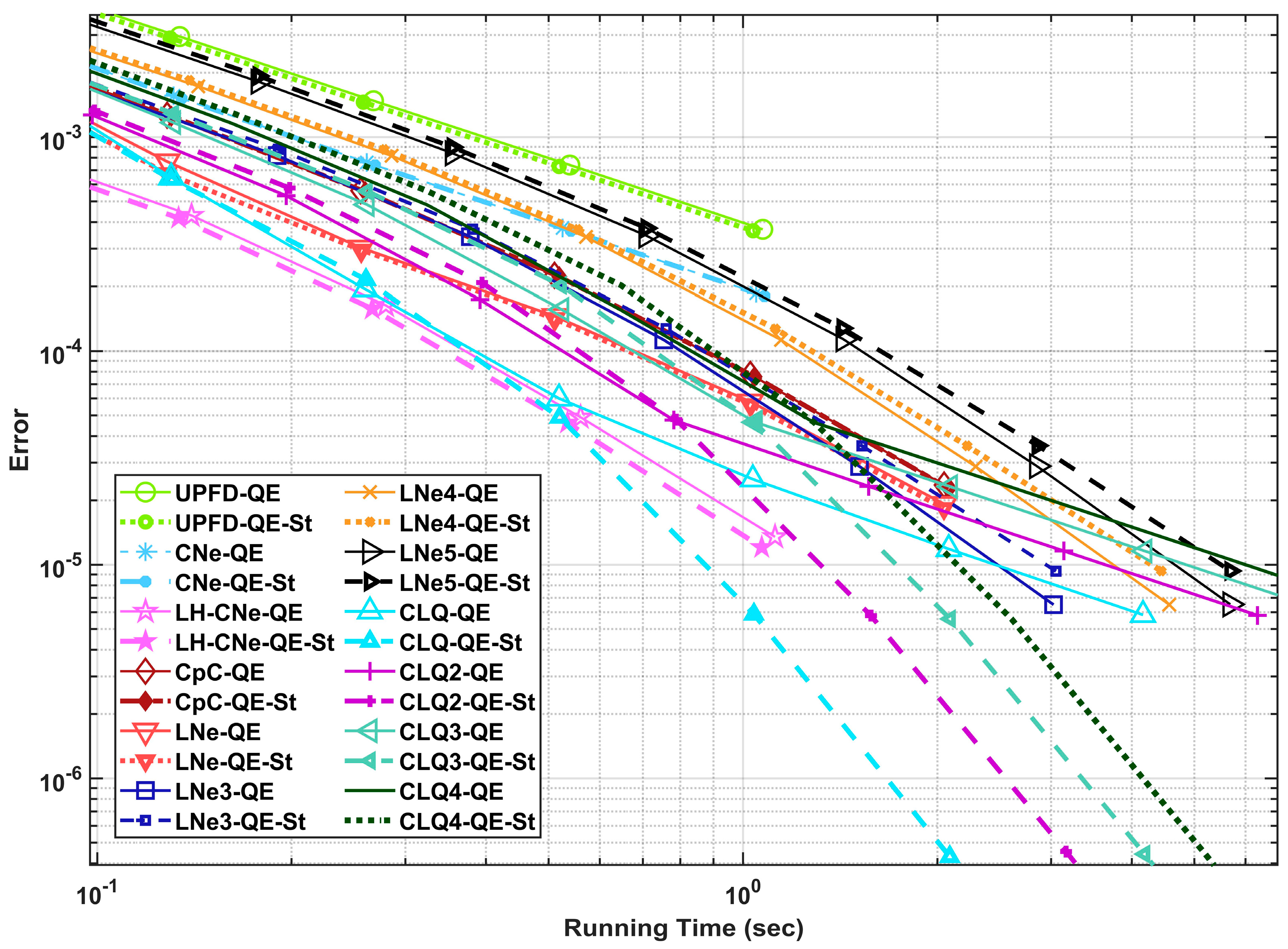
5.1. Experiment 2: Stiff System
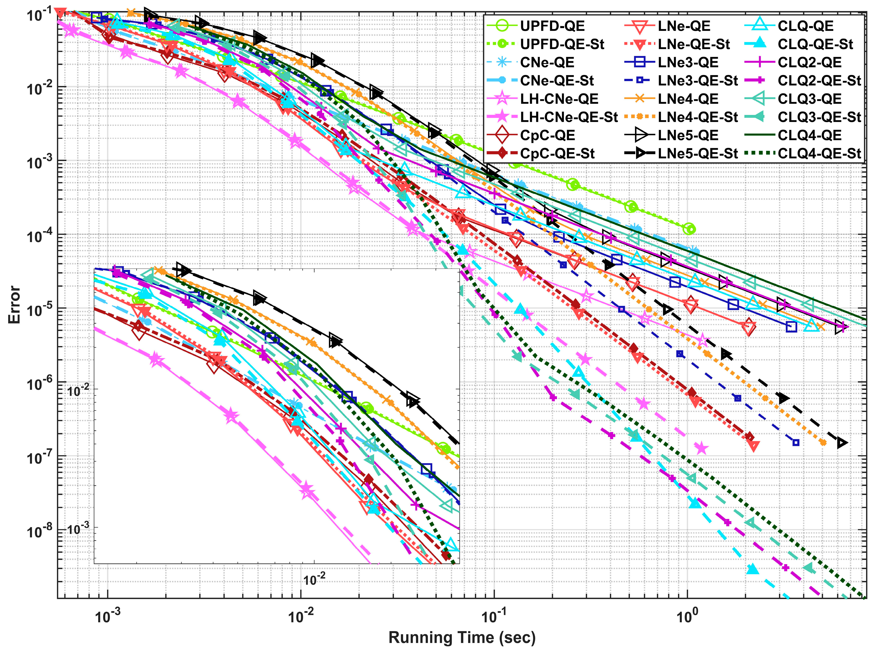
5.2. Experiment 2: Anysotropic System
6. Testing of Performance with Parameter Sweep for the Top 10 Methods
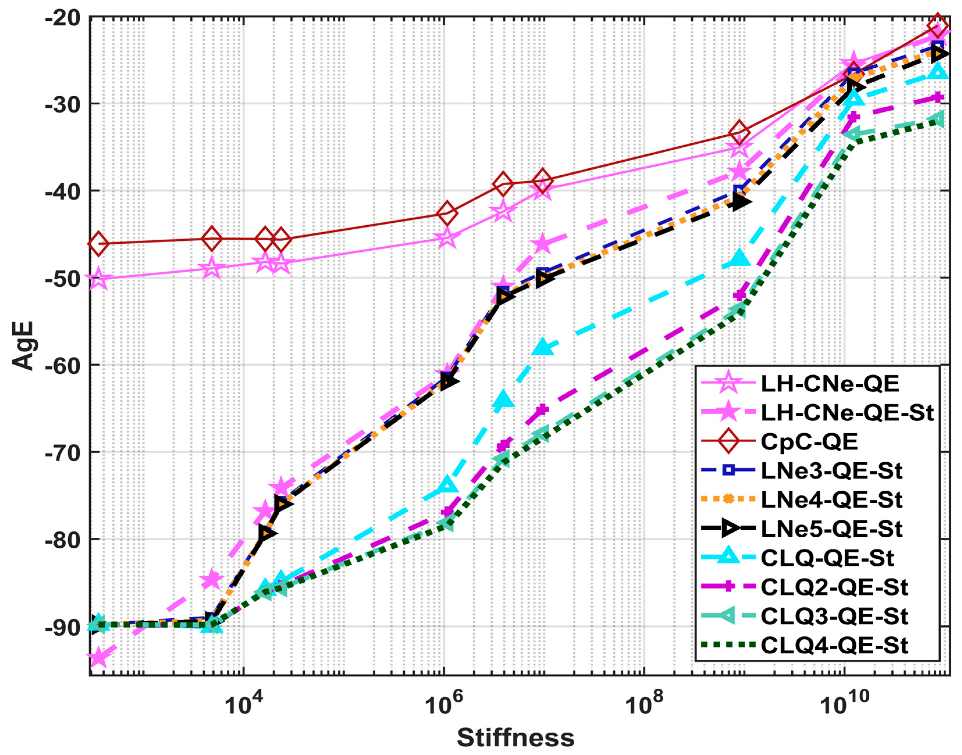
6.1. Comparison of the AgE Errors as Functions of the Stiffness Ratios
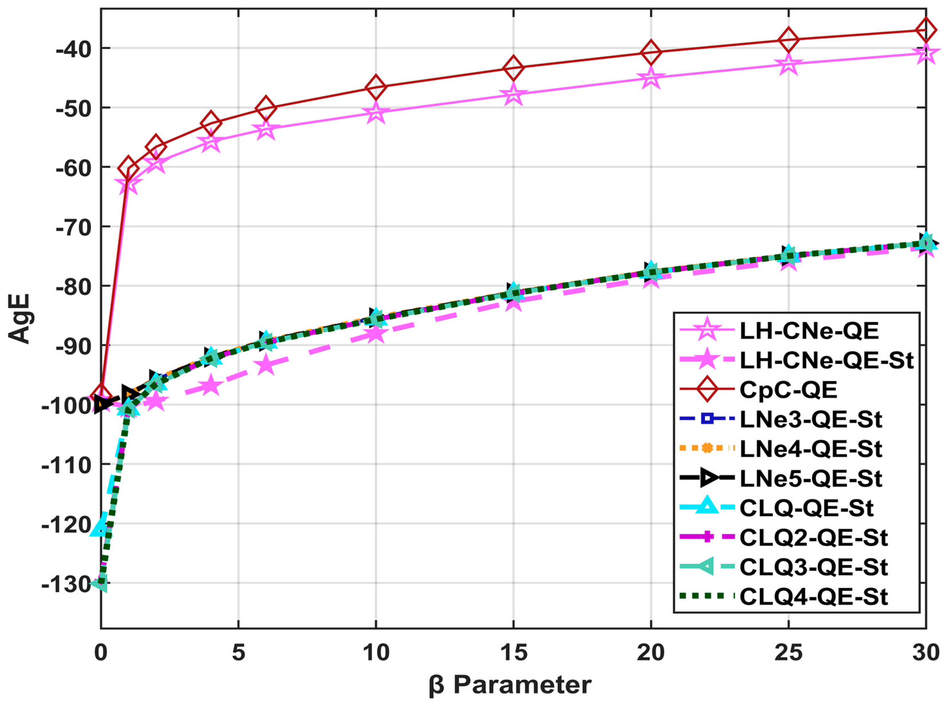
6.2. Comparison of the AgE Errors as Functions of the β Parameter
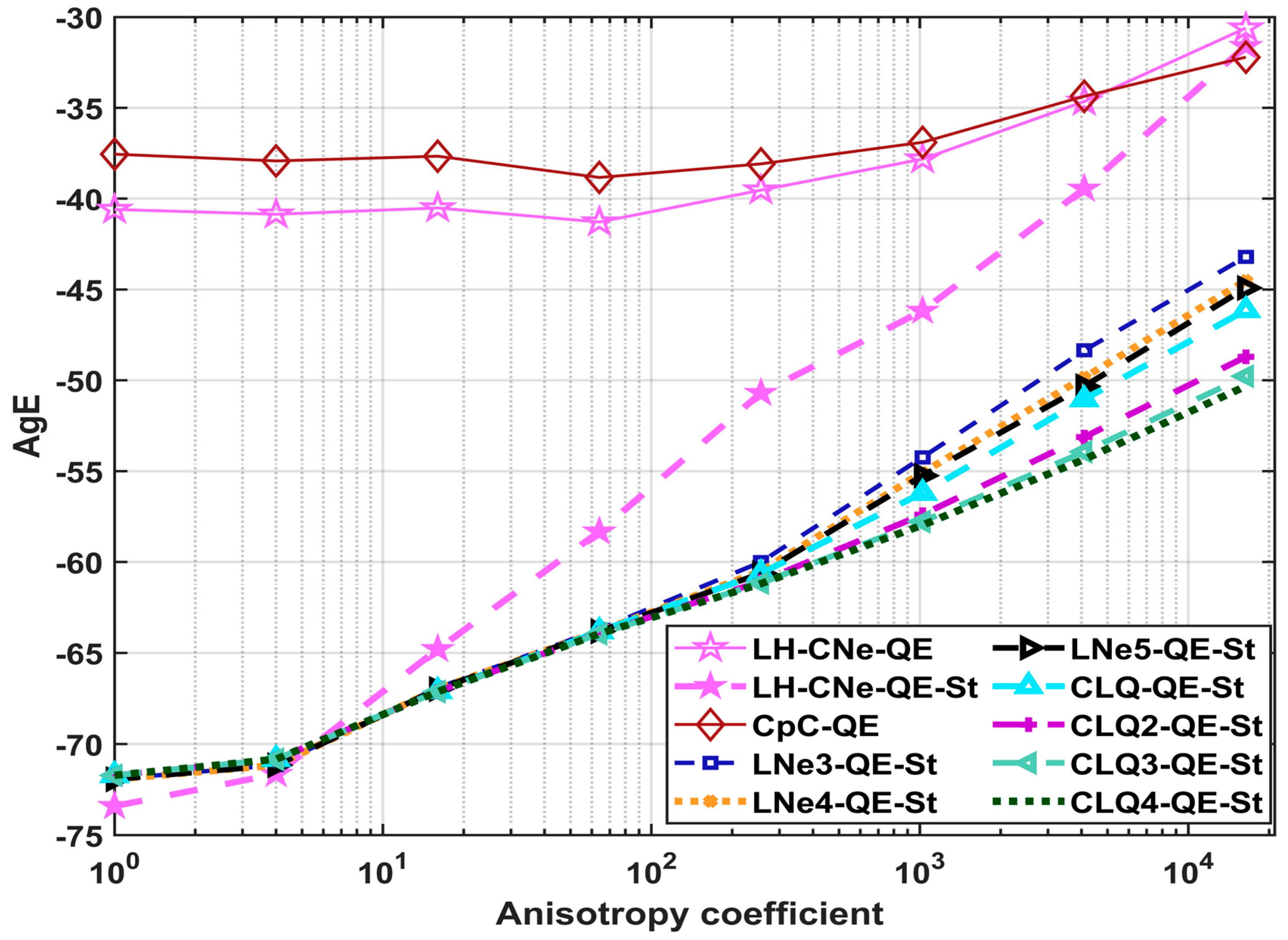
6.3. Comparison of the AgE Errors as Functions of the Anisotropy Coefficients (ACs)
7. Discussion and Conclusions
Author Contributions
Funding
Data Availability Statement
Conflicts of Interest
Appendix A
References
- Li, Y.; van Heijster, P.; Marangell, R.; Simpson, M.J. Travelling wave solutions in a negative nonlinear diffusion–reaction model. J. Math. Biol. 2020, 81, 1495–1522. [Google Scholar] [CrossRef]
- Weickenmeier, J.; Jucker, M.; Goriely, A.; Kuhl, E. A physics-based model explains the prion-like features of neurodegeneration in Alzheimer’s disease, Parkinson’s disease, and amyotrophic lateral sclerosis. J. Mech. Phys. Solids 2019, 124, 264–281. [Google Scholar] [CrossRef]
- Campos, D.; Llebot, J.E.; Fort, J. Reaction–diffusion pulses: A combustion model. J. Phys. A Math. Gen. 2004, 37, 6609–6621. [Google Scholar] [CrossRef]
- Columbu, A.; Frassu, S.; Viglialoro, G. Refined criteria toward boundedness in an attraction–repulsion chemotaxis system with nonlinear productions. Appl. Anal. 2024, 103, 415–431. [Google Scholar] [CrossRef]
- Li, T.; Frassu, S.; Viglialoro, G. Combining effects ensuring boundedness in an attraction–repulsion chemotaxis model with production and consumption. Z. Angew. Math. Phys. 2023, 74, 109. [Google Scholar] [CrossRef]
- Ma, W.; Fuchssteiner, B. Explicit and exact solutions to a Kolmogorov-Petrovskii-Piskunov equation. Int. J. Non-Linear Mech. 1996, 31, 329–338. [Google Scholar] [CrossRef]
- Hammond, J.F.; Bortz, D.M. Analytical solutions to Fisher’s equation with time-variable coefficients. Appl. Math. Comput. 2011, 218, 2497–2508. [Google Scholar] [CrossRef]
- Bastani, M.; Salkuyeh, D.K. A highly accurate method to solve Fisher’s equation. Pramana 2012, 78, 335–346. [Google Scholar] [CrossRef]
- Agbavon, K.M.; Appadu, A.R.; Khumalo, M. On the numerical solution of Fisher’s equation with coefficient of diffusion term much smaller than coefficient of reaction term. Adv. Differ. Equ. 2019, 2019, 146. [Google Scholar] [CrossRef]
- Tang, S.; Weber, R.O. Numerical study of Fisher’s equation by a Petrov-Galerkin finite element method. J. Aust. Math. Soc. Ser. B Appl. Math. 1991, 33, 27–38. [Google Scholar] [CrossRef]
- Chandraker, V.; Awasthi, A.; Jayaraj, S. A Numerical Treatment of Fisher Equation. Procedia Eng. 2015, 127, 1256–1262. [Google Scholar] [CrossRef]
- Dag, I.; Ersoy, O. The exponential cubic B-spline algorithm for Fisher equation. Chaos Solitons Fractals 2016, 86, 101–106. [Google Scholar] [CrossRef]
- Tamsir, M.; Huntul, M. A numerical approach for solving Fisher’s reaction–diffusion equation via a new kind of spline functions. Ain Shams Eng. J. 2021, 12, 3157–3165. [Google Scholar] [CrossRef]
- Holmes, M.H. Introduction to Numerical Methods in Differential Equations; Springer: New York, NY, USA, 2007. [Google Scholar] [CrossRef]
- Anguelov, R.; Lubuma, J.M.-S.; Shillor, M.; Anguelov, R.; Lubuma, J.M.-S.; Shillor, M. Dynamically consistent nonstandard finite difference schemes for continuous dynamical systems. Conf. Publ. 2009, 2009, 34–43. [Google Scholar] [CrossRef]
- Chen-Charpentier, B.M.; Kojouharov, H.V. An unconditionally positivity preserving scheme for advection–diffusion reaction equations. Math. Comput. Model. 2013, 57, 2177–2185. [Google Scholar] [CrossRef]
- Appadu, A.R. Performance of UPFD scheme under some different regimes of advection, diffusion and reaction. Int. J. Numer. Methods Heat Fluid Flow 2017, 27, 1412–1429. [Google Scholar] [CrossRef]
- Drljača, B.; Savović, S. Unconditionally positive finite difference and standard explicit finite difference schemes for power flow equation. Univ. Thought-Publ. Nat. Sci. 2019, 9, 75–78. [Google Scholar] [CrossRef]
- Dimitrov, D.T.; Kojouharov, H.V. Positive and elementary stable nonstandard numerical methods with applications to predator–prey models. J. Comput. Appl. Math. 2006, 189, 98–108. [Google Scholar] [CrossRef]
- Chertock, A.; Kurganov, A. A second-order positivity preserving central-upwind scheme for chemotaxis and haptotaxis models. Numer. Math. 2008, 111, 169–205. [Google Scholar] [CrossRef]
- Agbavon, K.M.; Appadu, A.R. Construction and analysis of some nonstandard finite difference methods for the FitzHugh–Nagumo equation. Numer. Methods Partial. Differ. Equ. 2020, 36, 1145–1169. [Google Scholar] [CrossRef]
- Songolo, M.E. A Positivity-Preserving Nonstandard Finite Difference Scheme for Parabolic System with Cross-Diffusion Equations and Nonlocal Initial Conditions. Am. Sci. Res. J. Eng. Technol. Sci. 2016, 18, 252–258. [Google Scholar]
- Chapwanya, M.; Lubuma, J.M.-S.; Mickens, R.E. Positivity-preserving nonstandard finite difference schemes for cross-diffusion equations in biosciences. Comput. Math. Appl. 2014, 68, 1071–1082. [Google Scholar] [CrossRef]
- Omle, I.; Askar, A.H.; Kovács, E. Systematic testing of explicit positivity preserving algorithms for the heat-equation. J. Math. Comput. Sci. 2022, 12, 162. [Google Scholar] [CrossRef]
- Kovács, E.; Majár, J.; Saleh, M. Unconditionally Positive, Explicit, Fourth Order Method for the Diffusion- and Nagumo-Type Diffusion–Reaction Equations. J. Sci. Comput. 2024, 98, 39. [Google Scholar] [CrossRef]
- Murray, M.Y. Comprehensive Biotechnology, 2nd ed.; Elsevier: Amsterdam, The Netherlands, 2011; Volume 1–6, pp. 1–4729. [Google Scholar]
- Nagy, Á.; Majár, J.; Kovács, E. Consistency and Convergence Properties of 20 Recent and Old Numerical Schemes for the Diffusion Equation. Algorithms 2022, 15, 425. [Google Scholar] [CrossRef]
- Ramos, J. A piecewise time-linearized method for the logistic differential equation. Appl. Math. Comput. 1998, 93, 139–148. [Google Scholar] [CrossRef]


| Numerical Method | Treatment of the Nonlinear Term | |||||
|---|---|---|---|---|---|---|
| PI | QE | PI-St | QE-St | PI-QE-St | QE-PI-St | |
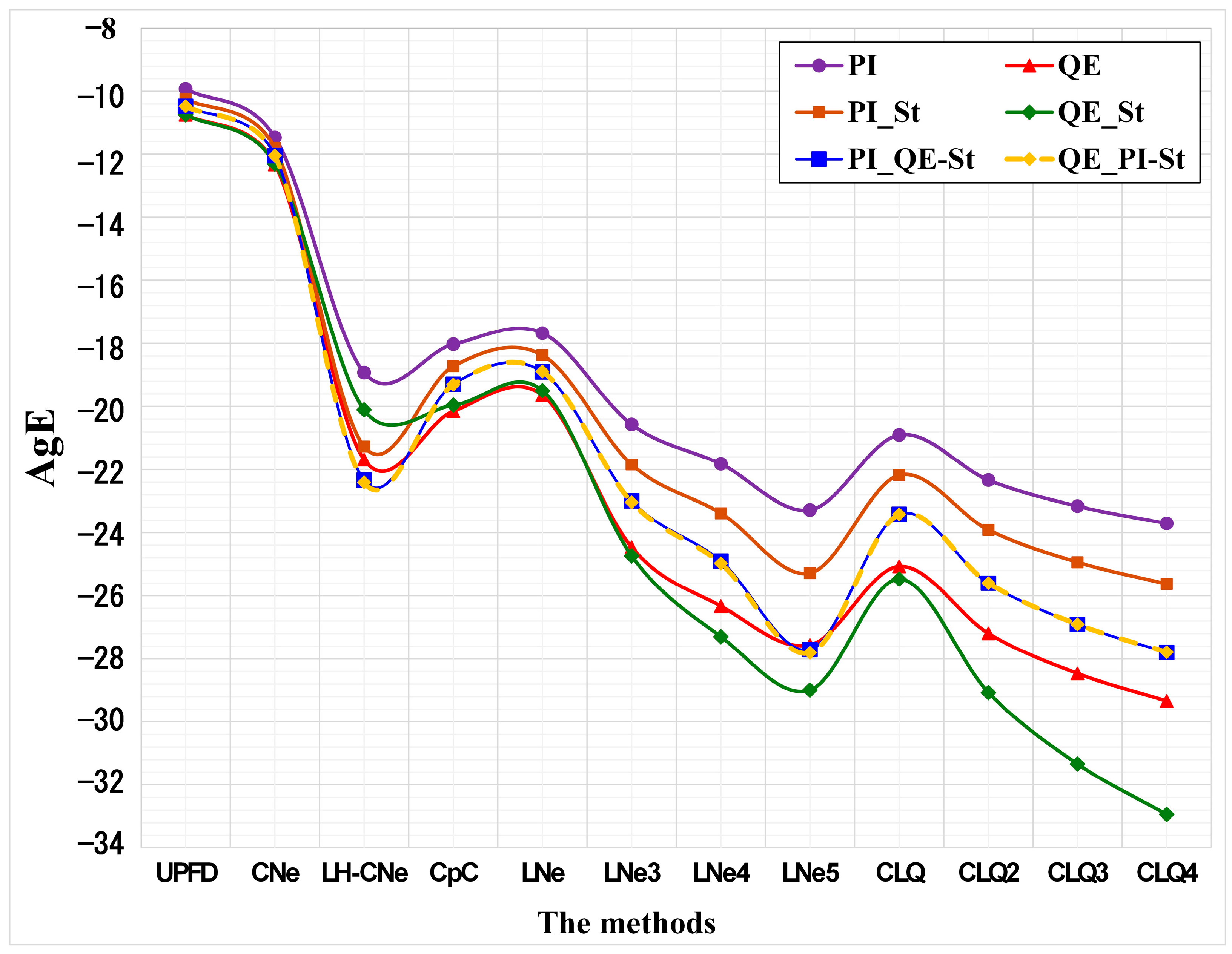
| UPFD | −9.93 | −10.74 | −10.25 | −10.74 | −10.48 | −10.48 |
| CNe | −11.46 | −12.32 | −11.80 | −12.31 | −12.043 | −12.04 |
| LH-CNe | −18.92 | −21.685 | −21.27 | −20.11 | −22.34 | −22.41 |
| CpC | −18.03 | −20.15 | −18.72 | −19.96 | −19.29 | −19.32 |
| LNe | −17.67 | −19.64 | −18.37 | −19.50 | −18.90 | −18.89 |
| LNe3 | −20.57 | −24.47 | −21.84 | −24.74 | −22.99 | −23.03 |
| LNe4 | −21.82 | −26.33 | −23.38 | −27.30 | −24.90 | −24.98 |
| LNe5 | −23.28 | −27.56 | −25.28 | −28.99 | −27.71 | −27.81 |
| CLQ | −20.90 | −25.07 | −22.18 | −25.47 | −23.42 | −23.42 |
| CLQ2 | −22.33 | −27.19 | −23.92 | −29.07 | −25.61 | −25.61 |
| CLQ3 | −23.16 | −28.47 | −24.94 | −31.34 | −26.91 | −26.91 |
| CLQ4 | −23.71 | −29.34 | −25.63 | −32.94 | −27.81 | −27.79 |
| Number | Type | ac | bc | aRX | bRx | aRz | bRz | Stiffness Ratios | hMax |
|---|---|---|---|---|---|---|---|---|---|
| 1 | Non Stiff | 0 | 0 | 0 | 0 | 0 | 0 | 356 | 0.251 |
| 2 | −1 | 1 | 0 | 0 | 0 | 0 | 4806.8 | 0.048 | |
| 3 | Mildly Stiff | −1 | 1 | −1 | 1 | 0 | 0 | 1.64 × 10⁴ | 0.012 |
| 4 | −1 | 1 | −1 | 1 | −1 | 1 | 2.36 × 10⁴ | 0.007 | |
| 5 | Moderately Stiff | −2 | 2 | −1 | 1 | −1 | 1 | 1.11 × 10⁶ | 0.001 |
| 6 | −2 | 2 | −2 | 2 | −1 | 1 | 3.92 × 10⁶ | 2.98 × 10⁻⁴ | |
| 7 | −2 | 2 | −2 | 2 | −2 | 2 | 9.74 × 10⁶ | 1.45 × 10⁻⁴ | |
| 8 | Very Stiff | −3 | 3 | −2 | 2 | −2 | 2 | 8.97 × 10⁸ | 2.04 × 10⁻⁵ |
| 9 | −3 | 3 | −3 | 3 | −2 | 2 | 1.34 × 10¹⁰ | 1.48 × 10⁻⁶ | |
| 10 | −3 | 3 | −3 | 3 | −3 | 3 | 8.56 × 10¹⁰ | 1.48 × 10⁻⁶ |
| Algorithms | The Stiffness Values | |||||||||
|---|---|---|---|---|---|---|---|---|---|---|
| 356 | 4806.8 | 1.6 × 10⁴ | 2.4 × 10⁴ | 1.1 × 10⁶ | 3.9 × 10⁶ | 9.7 × 10⁶ | 8.9 × 10⁸ | 1.3 × 10¹⁰ | 8.5 × 10¹⁰ | |
| AgE Errors | ||||||||||
| LH-CNe-QE | −50.18 | −48.94 | −48.20 | −48.36 | −45.42 | −42.39 | −39.90 | −35.03 | −25.41 | −22.08 |
| LH-CNe-QE-St | −93.60 | −84.68 | −76.80 | −74.15 | −61.08 | −51.02 | −46.17 | −37.83 | −25.72 | −22.21 |
| CpC-QE | −46.11 | −45.52 | −45.55 | −45.63 | −42.61 | −39.25 | −38.87 | −33.33 | −26.64 | −21.05 |
| LNe3-QE-St | −89.78 | −88.97 | −79.07 | −75.70 | −61.40 | −51.58 | −49.43 | −39.96 | −26.50 | −23.40 |
| LNe4-QE-St | −89.80 | −89.34 | −79.31 | −75.96 | −61.82 | −51.99 | −49.97 | −40.76 | −27.05 | −24.01 |
| LNe5-QE-St | −89.80 | −89.41 | −79.35 | −76.00 | −61.90 | −52.19 | −50.14 | −41.28 | −28.14 | −24.28 |
| CLQ-QE-St | −89.76 | −89.99 | −85.79 | −84.86 | −73.93 | −64.14 | −58.19 | −47.9 | −29.52 | −26.51 |
| CLQ2-QE-St | −89.77 | −89.86 | −86.03 | −85.36 | −76.92 | −69.28 | −65.11 | −52.04 | −31.52 | −29.27 |
| CLQ3-QE-St | −89.77 | −89.81 | −86.03 | −85.57 | −78.15 | −70.77 | −67.88 | −53.59 | −33.56 | −31.76 |
| CLQ4-QE-St | −89.77 | −89.80 | −86.04 | −85.59 | −78.48 | −71.23 | −68.40 | −54.16 | −34.50 | −32.08 |
| Rx | 1 | 2 | 4 | 8 | 16 | 32 | 64 | 128 |
| Rz | 1 | 1/2 | 1/4 | 1/8 | 1/16 | 1/32 | 1/64 | 1/128 |
| A.C. | 1 | 4 | 16 | 64 | 256 | 1024 | 4096 | 16,384 |
| Algorithms | AgE Errors | |||||||
| LH-CNe-QE | −40.594 | −40.858 | −40.511 | −41.287 | −39.53 | −37.822 | −34.651 | −30.609 |
| LH-CNe-QE-St | −73.404 | −71.645 | −64.797 | −58.332 | −50.699 | −46.178 | −39.455 | −31.602 |
| CpC-QE | −37.551 | −37.922 | −37.662 | −38.833 | −38.085 | −36.896 | −34.363 | −32.209 |
| LNe3-QE-St | −71.916 | −71.156 | −66.913 | −63.708 | −60.004 | −54.236 | −48.351 | −43.201 |
| LNe4-QE-St | −71.933 | −71.163 | −66.973 | −63.82 | −60.507 | −55.078 | −49.844 | −44.516 |
| LNe5-QE-St | −71.933 | −71.163 | −66.988 | −63.818 | −60.624 | −55.251 | −50.331 | −44.917 |
| CLQ-QE-St | −71.706 | −70.835 | −67.107 | −63.826 | −60.625 | −56.201 | −51.046 | −46.136 |
| CLQ2-QE-St | −71.717 | −70.833 | −67.125 | −63.936 | −61.068 | −57.393 | −53.127 | −48.703 |
| CLQ3-QE-St | −71.717 | −70.832 | −67.125 | −63.95 | −61.163 | −57.778 | −53.932 | −49.774 |
| CLQ4-QE-St | −71.717 | −70.832 | −67.125 | −63.954 | −61.195 | −57.968 | −54.356 | −50.324 |
Disclaimer/Publisher’s Note: The statements, opinions and data contained in all publications are solely those of the individual author(s) and contributor(s) and not of MDPI and/or the editor(s). MDPI and/or the editor(s) disclaim responsibility for any injury to people or property resulting from any ideas, methods, instructions or products referred to in the content. |
© 2024 by the authors. Licensee MDPI, Basel, Switzerland. This article is an open access article distributed under the terms and conditions of the Creative Commons Attribution (CC BY) license (https://creativecommons.org/licenses/by/4.0/).
Share and Cite
Khayrullaev, H.; Omle, I.; Kovács, E. Systematic Investigation of the Explicit, Dynamically Consistent Methods for Fisher’s Equation. Computation 2024, 12, 49. https://doi.org/10.3390/computation12030049
Khayrullaev H, Omle I, Kovács E. Systematic Investigation of the Explicit, Dynamically Consistent Methods for Fisher’s Equation. Computation. 2024; 12(3):49. https://doi.org/10.3390/computation12030049
Chicago/Turabian StyleKhayrullaev, Husniddin, Issa Omle, and Endre Kovács. 2024. "Systematic Investigation of the Explicit, Dynamically Consistent Methods for Fisher’s Equation" Computation 12, no. 3: 49. https://doi.org/10.3390/computation12030049
APA StyleKhayrullaev, H., Omle, I., & Kovács, E. (2024). Systematic Investigation of the Explicit, Dynamically Consistent Methods for Fisher’s Equation. Computation, 12(3), 49. https://doi.org/10.3390/computation12030049