A Novel Megastable Chaotic System with Hidden Attractors and Its Parameter Estimation Using the Sparrow Search Algorithm

Abstract

This work proposes a new two-dimensional dynamical system with complete nonlinearity. This system inherits its nonlinearity from trigonometric and hyperbolic functions like sine, cosine, and hyperbolic sine functions. This system gives birth to infinite but countable coexisting attractors before and after being forced. These two megastable systems differ in the coexisting attractors’ type. Only limit cycles are possible in the autonomous version, but torus and chaotic attractors can emerge after transforming to the nonautonomous version. Because of the position of equilibrium points in different attractors’ attraction basins, this system can simultaneously exhibit self-excited and hidden coexisting attractors. This system’s dynamic behaviors are studied using state space, bifurcation diagram, Lyapunov exponents (LEs) spectrum, and attraction basins. Finally, the forcing term’s amplitude and frequency are unknown parameters that need to be found. The sparrow search algorithm (SSA) is used to estimate these parameters, and the cost function is designed based on the proposed system’s return map. The simulation results show this algorithm’s effectiveness in identifying and estimating parameters of the novel megastable chaotic system.

1. Introduction

Thirty years after Sprott struggled to find the most straightforward chaotic systems [1], there is still interest in finding new chaotic (or, in general, dynamical) systems with unique features [2]. A category of nonlinear dynamical systems is multistable systems [3]. In multistable systems, there is more than one attractor that the system’s trajectory can converge to [3]. The selection between different attractors only depends on the trajectory starting points; in other words, the dependence is on the system’s initial conditions and not the parameters. These attractors are called coexisting attractors [4,5]. Each attractor has its attraction basin; if the chosen initial condition falls in this region, the corresponding attractor will appear in the state space [4]. A subset of multistable systems belongs to megastable systems [6]. The property of these systems is that although they possess infinite coexisting attractors, they can be distinguished from each other and are countable [6]. This distinguishability is because their attraction basin presents a nested pattern [6]. Consequently, when considering the initial condition as the bifurcation parameter, each attractor is visited at specific intervals and then jumps to the neighboring attractor. This phenomenon causes a step-like pattern in their initial condition-dependent bifurcation diagrams.

Another property of such systems that attract the attention of researchers is the nested coexisting attractors that can present exciting patterns [7] like the objects around us [8,9]. Classically, megastability has been observed in forced nonlinear systems, which are also known as nonautonomous systems [6]. The forcing function can be selected from various mathematical expressions [10,11]; for instance, it can be periodic or quasi-periodic [12,13]. Recently, some studies have proposed unforced autonomous megastable systems [14,15]. From the energy consumption viewpoint, like any other nonlinear dynamical system, megastable systems can be dissipative or conservative [16,17]; there are some exceptional cases in which the system’s megastability relies on its Hamiltonian energy [15]. Megastability has also been observed in memristor-based [15,16] and delayed systems [13]. What makes studying megastability vital is that this feature has been reported in artificially designed sets of differential equations and systems representing the dynamics of the natural world and physical phenomena such as single-link manipulators [12] and Josephson junction snap oscillators [18]. Even artificially designed megastable systems, because of their various dynamics, can be applied in many engineering fields, such as image encryption and signal protection, which are especially crucial in medical environments to protect the privacy and security of patients [5,14,18].

For many years, it has been assumed that the system’s initial conditions should be chosen near its equilibrium point to find an attractor. Thus, all attractors can be discovered straightforwardly. Nevertheless, the concept of hidden attractors was introduced in 2011 [19]. These attractors are named hidden because no equilibrium point in their attraction basin helps to locate them [19]. As a result, the classic attractors with equilibrium points in their attraction basins have been called self-excited and the rest are hidden [19]. It may be considered that only systems without any equilibrium points [20,21,22] can show hidden attractors; however, it should be noted that systems with one stable equilibrium point [23], line [24], and the surfaces of equilibrium points [25] also represent hidden attractors. The reason is that, despite equilibrium points in such systems, they do not make the discovery of attractors easier. Chua’s circuit is the most famous example of a chaotic system with a hidden attractor [26]. Recently, some modifications have been made to the classic Chua circuit, and hidden attractors in these new versions have also been reported [27]. Apart from the classic example of Chua’s circuit, such attractors have been reported in other kinds of systems such as memristor [28,29,30] or meminductor-based [31] and fractional order [21,30,32,33] systems. Notably, a system can possess self-excited and hidden attractors simultaneously [33,34,35]; recently, the concept of hidden attractors has been leveraged to include strange nonchaotic attractors as well [36]. Searching for hidden attractors is computationally exhaustive, but some methods, like offset boosting [37], variable boosting [38], and connecting curves [39] have been introduced to make this procedure easier. After the first hidden attractor discovery, scientists have attempted to find other examples, most of which are based on systems representing physical or biological phenomena like dark energy and dark matter [32], plasma [40], quadrotor crewless aerial vehicles [41], the Moore–Spiegel system [42], the Hindmarsh–Rose neuron model [28] and the Hopfield neural network [29]. Because of the complexity of locating hidden attractors rather than self-excited ones, the chaotic systems with such attractors are potential candidates in image encryption [22,34,35], random number generation [35], and weak signal detection [43] in the engineering world.

Optimization algorithms have become an essential intelligence tool in almost all engineering fields [44]. Optimization is a process followed to make something better. A thought, idea, or design that a scientist or an engineer proposes is improved during the optimization process. During optimization, initial conditions are examined by various methods, and the information obtained is used to improve an idea or method. Optimization algorithms can be used to identify the chaotic systems’ unknown parameters [45]. Parameter estimation for chaotic systems is one of the most critical issues in nonlinear science [46]. A chaotic system parameter estimation problem can be expressed as a multivariate optimization problem; the optimization algorithm estimates the system parameters [47]. The algorithm finds the unknown parameters’ best value to obtain the objective function minimum value [48,49]. One of the new optimization algorithms is the sparrow search algorithm (SSA), which is modeled after the behavior of sparrows [50]. The SSA has been applied as a powerful and robust algorithm to search for the optimal response of the objective function [50].

This paper proposes a novel chaotic megastable system with an infinite but countable number of hidden coexisting attractors.

This work can be considered novel in many aspects; some of the most important aspects are highlighted here. First, among the cost functions that can be used for the parameter identification of chaotic systems, the one based on return maps similarity [51] is more reliable and robust against the intrinsic characteristic of such systems, which is the sensitivity to initial conditions. To the authors’ best knowledge, the capability of this cost function has never been examined in the parameter estimation of megastable chaotic systems. The presence of infinite coexisting attractors in such systems makes the design of suitable cost functions essential. Therefore, in this work, despite reporting the proposed megastable system for the first time, employing the above-mentioned cost function for its parameter identification is another new approach. Second, although the strength of the SSA in solving many optimization problems has been demonstrated, to the authors’ best knowledge, it has never been applied to the parameter estimation of megastable chaotic systems that could have more challenging cost functions with several local minima and abrupt changes, which necessitate the use of more powerful optimization algorithms.

Consequently, the selection of this algorithm is also novel. The results of this research can expand the practical application of the cost function based on return maps to multistable chaotic systems with infinite coexisting attractors. Its performance on extreme multistable, super-extreme multistable, and mega-extreme multistable chaotic systems can be considered in the future. In addition, since optimization algorithms evolve continuously, the ability of a recently introduced algorithm in the parameter identification of chaotic systems can be signified. This makes SSA a new candidate for the parameter estimation of chaotic and hyperchaotic systems with a single, or several coexisting, attractors.

Motivated by the cost function designed based on the similarity between return maps [51], and after studying the chaotic systems whose parameters have been identified using this approach, we have designed a new two-dimensional megastable chaotic system to test the ability of this technique in chaotic systems with more complicated dynamics and several coexisting attractors. After becoming familiar with the SSA algorithm and confirming its ability to solve many complex optimization problems, we were eager to employ it as the optimization algorithm for our problem of megastable chaotic system identification. We were curious to analyze the collaboration between the mentioned cost function and the SSA. In order to fill these research gaps, the contributions of this paper can be listed as follows:

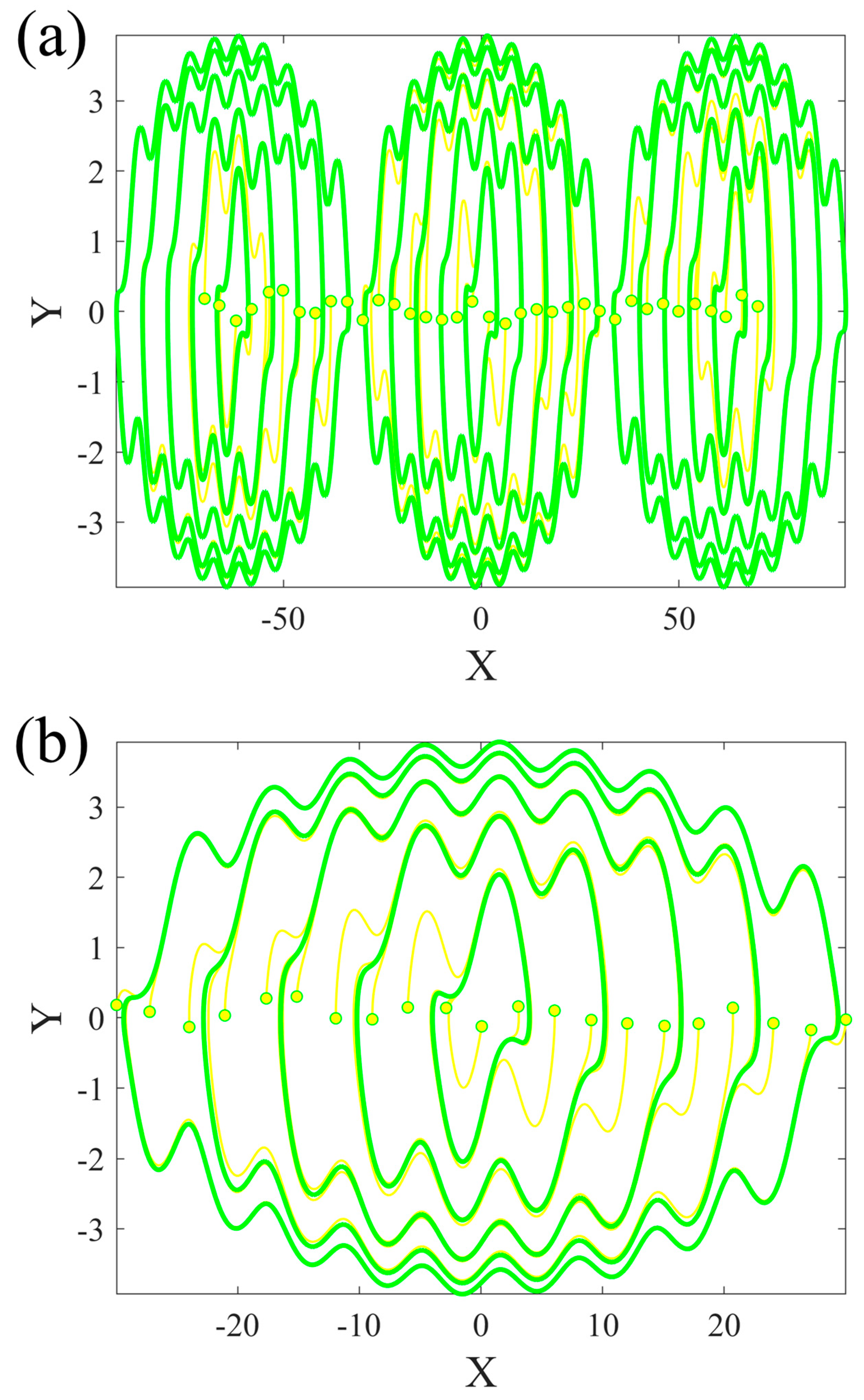
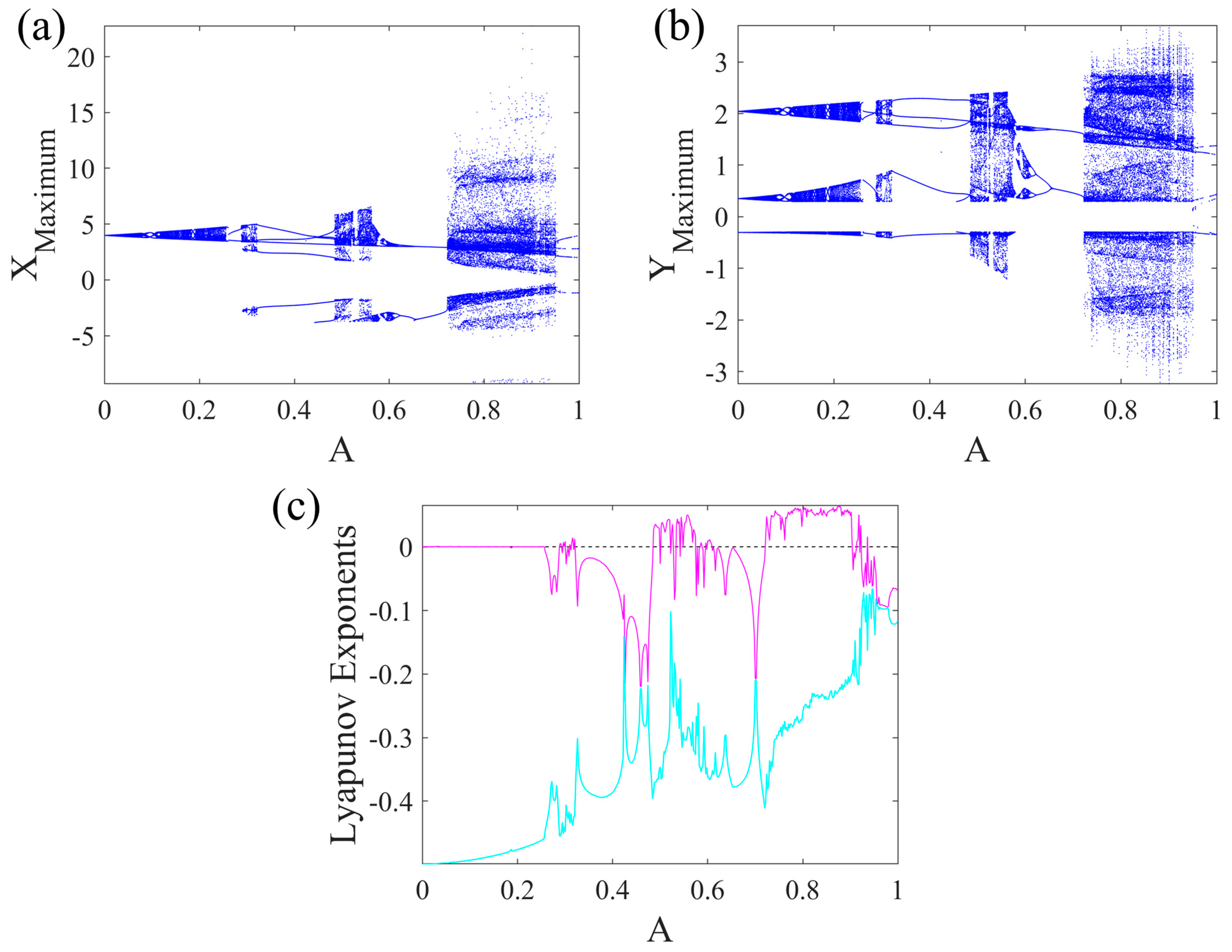
• Designing a new chaotic megastable system with hidden attractors and studying its dynamics by plotting the phase portraits of coexisting attractors, their attraction basin, bifurcation diagrams, and Lyapunov exponents spectrum;
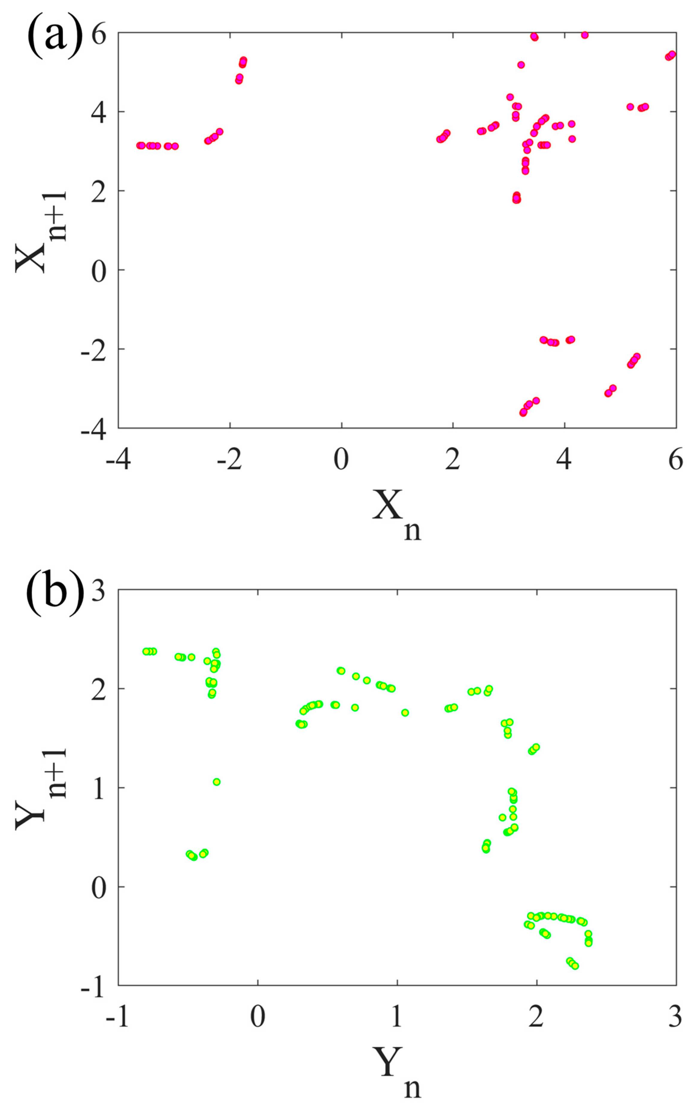
• Forming the cost function based on the similarity between the return maps obtained from the $x$ time series;
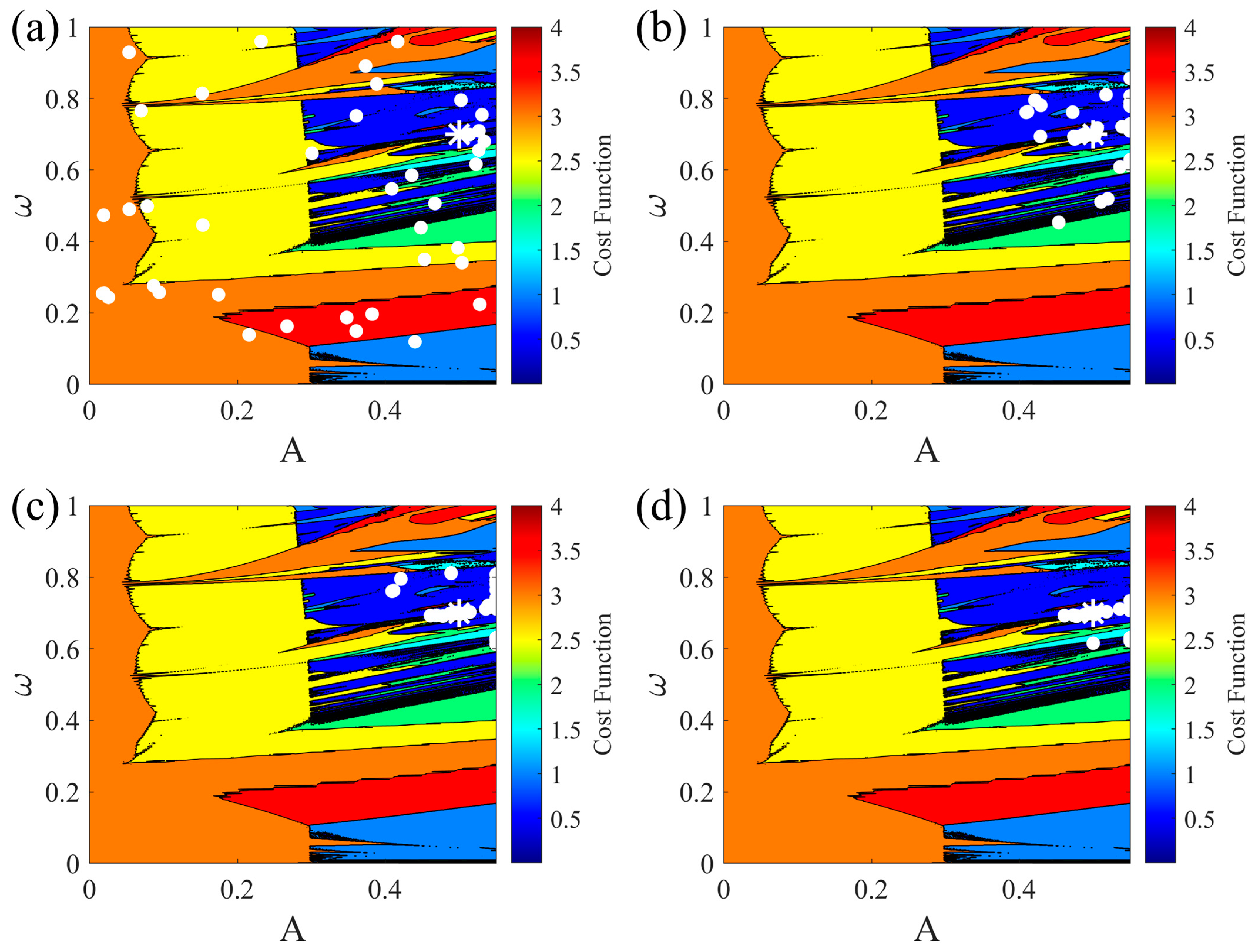
• Setting the amplitude and frequency of the sinusoidal forcing term as the unknown parameters and attempting to discover them with the help of the cost function on the previous step and the SSA.

The paper’s layout is as follows: The proposed system dynamics before and after applying the forcing function are thoroughly analyzed in Section 2. The unforced system symmetry and equilibrium points are studied in this section. Moreover, the coexisting attractors and their attraction basins in the unforced and forced systems are reported alongside the bifurcation diagrams and LEs spectrum after being forced. The SSA estimates two forcing term parameters, amplitude and frequency, and a cost function based on the system’s return map, which is designed in Section 3. The cost function at each iteration and the sparrows’ position evolution are reported in this section. The paper is then summarized and briefly explained in Section 4.

2. The Megastable Chaotic System

This part introduces a new two-dimensional autonomous megastable system as System (1).

$$\begin{array}{l}\dot{x}=\sinh \left(y\right)\\ \dot{y}=-\sin \left(0.1x\right)+y\cos \left(x\right)\end{array}$$

(1)

System (1) is fully nonlinear and composed of hyperbolic and trigonometric functions such as sine, cosine, and hyperbolic sine functions. This system is symmetric around the origin because its equations do not change when $\left(x,y\right)\to \left(-x,-y\right)$, which results in symmetric attractors (or symmetric coexisting attractors). System (1) has infinite symmetric coexisting limit cycle groups, as shown in Figure 1. Each group consists of five symmetric limit cycles. These symmetric coexisting limit cycles’ initial conditions are chosen randomly around the $y$ axis and are depicted by yellow circles. The transient and steady-state parts are plotted in yellow and green. This system has an infinite number of equilibrium points located on the $x$-axis at $\left[10n\pi ,0\right], n\in \mathbb{Z}$, which are presented by red circles in Figure 2 for $n\in \{-3,-2,-\mathrm{1,0},\mathrm{1,2},3\}$. The attraction basin for the central group of symmetric coexisting limit cycles is also portrayed in this figure. Yellow represents the initial conditions that cause the innermost limit cycle to appear; by growing the limit cycle size, the color tends to be blue. The dark blue region corresponds to the initial conditions associated with the limit cycles outside the central group. Each group’s innermost and outermost limit cycles are self-excited (their attraction basins contain at least one equilibrium point), while the three middle limit cycles are hidden by definition. Therefore, System (1) possesses self-excited and hidden attractors at the same time.

Adding a periodic driving force to System (1), a two-dimensional nonautonomous megastable system is achieved as System (2), as follows:

$$\begin{array}{l}\dot{x}=\sinh \left(y\right)+A\mathrm{s}\mathrm{i}\mathrm{n}\left(\omega t\right)\\ \dot{y}=-\sin \left(0.1x\right)+y\cos \left(x\right)\end{array}$$

(2)

$A$ and $\omega$ stand for the periodic driving force amplitude and frequency. System (2) has no equilibrium point; therefore, all its coexisting attractors belong to the hidden category. In order to find more complex dynamics other than the limit cycle, such as torus and chaos in System (2), many combinations of $\left(A,\omega \right)$ were tested by trial and error. Selecting$\omega =0.7$, amplitude $A$ is considered as the bifurcation parameter in the $\left[\mathrm{0,1}\right]$ interval. It is shown that this bifurcation parameter can result in different dynamical solutions. The central attractor bifurcation and Lyapunov exponents (LEs) diagram is illustrated in Figure 3. The bifurcation diagrams are attained by plotting the $x$ and $y$ time series local maximum values. Although they present consistent behaviors in an identical bifurcation parameter, plotting them side by side makes it easier to imagine that the space occupied by the attractor. For small values of $A$ ($A\in \left[\mathrm{0,0.254}\right]$), the dynamical solution is a torus. The ordered pattern of the bifurcation diagrams in this interval can highlight this behavior. In contrast, for higher values of $A$, periodic and chaotic solutions can also be detected. The period doubling, period halving, and crisis can be detected in the bifurcation diagrams. The observable crises are interior and exterior ones. An interior crisis, known as an explosive bifurcation, occurs when the attractor’s shape or size changes abruptly. On the other hand, an exterior or boundary crisis is when a chaotic attractor emerges or vanishes suddenly. It should be noted that increasing the bifurcation parameter constantly makes the attractor size more prominent in the entire interval. In addition, compared to System (1), periodic solutions can have periods higher than one; several periodic windows are observable in the chaotic zones. The LEs confirm the behaviors observed in the bifurcation diagrams. One of the LEs is always negative, demonstrated in cyan, and the other can be positive, zero, or negative, as plotted in magenta. When System (2) converges to periodic, torus, and chaotic solutions, the magenta LE becomes negative, zero, and positive. A black dashed line shows the zero line; the magenta LE touches it at the bifurcation points. As can be inferred from Figure 3, the absolute value of the negative LE is always larger than the positive one. Because the sum of all LEs quantifies the system’s dissipativity, it can be concluded that the sum of LEs is always negative; hence, for the selected parameters and initial conditions, the system is dissipative and all trajectories are attractors.

Choosing $A=0.2$ in the bifurcation diagrams torus area and keeping $\omega =0.7$, interestingly, some of the previous five limit cycles have been merged and formed four torus attractors. These four central torus attractors with their attraction basins are presented in Figure 4. Yellow represents the initial conditions that cause the innermost attractor to appear; by growing the attractor size, the color tends to be blue. The dark blue region corresponds to the initial conditions associated with the attractors outside the central group.

Choosing $A=0.5$ in the bifurcation diagrams chaotic area and keeping $\omega =0.7$, some of the previous five limit cycles have been merged and formed four attractors. Surprisingly, there are three chaotic and one limit cycle attractors now. These four central coexisting attractors with their attraction basins are presented in Figure 5. Yellow represents the initial conditions that cause the innermost attractor to appear; by growing the attractor size, the color tends to be blue. The dark blue region corresponds to the initial conditions associated with the attractors outside the central group.

3. Cost Function and Parameter Estimation

The parameter estimation of chaotic systems, and, especially, megastable systems is challenging because a slight error can result in completely wrong answers. Consider a chaotic system with unknown parameters where only its time series is accessible. In order to find the unknown parameters, an optimization algorithm should be deployed; before that, a cost function should be introduced. The optimization algorithm aims to discover the parameter values for which the cost function becomes the least. Such cost functions are usually designed based on similarity indices. In nonchaotic systems, this cost function can be stated in terms of the difference between the model and system time series. However, because of the sensitivity to initial conditions in chaotic systems, such time domain-based cost functions are ineffective. In other words, the model and the system can have similar parameters but different initial conditions that lead to entirely different time series. On the other hand, they have similar patterns in the phase space.

In 2014, a cost function was introduced to solve the parameter estimation problem in chaotic systems [51]. This method does not directly compare the system and model time series, but their return maps are used. This means that their local maxima are found and form a sequence after their time series are obtained. The return map states each sample of this sequence depending on its previous sample. Thus, it is a recursive method that defines its name well. It should be noted that the local maxima are found after removing enough transient parts. The return maps of System (2) with $A=0.5$, $\omega =0.7$, and initial conditions $\left(x_0,y_0\right)=\left(\mathrm{0.1,0}\right),$ based on both $x$ and $y$ time series, are portrayed in Figure 6. The irregular pattern of the points in both return maps without uniform density confirms the chaotic behavior of System (2) for these parameter sets that agrees with the discussions in the previous section.

Assume that the points number in the system and the model sequences are $L_s$ and $L_m$, respectively. In the proposed cost function, at first, the distance between points ($D$) is set to zero. Then, two loops occur: one for the system ($i=1$ to $L_s$) and one for the model ($j=1$ to $L_m$). At each iteration of the system loop, the Euclidean distance between the $i$th system data point and all model data points is calculated. The minimum value among them is selected as $d_i$ and $D$ is updated as $D=D+d_i$. The model loop starts after the system loop ends, and a similar procedure is performed. At each step, the nearest system data point to the $j$th model data point is considered as $d_j$ and $D$ is changed as $D=D+d_j$. Finally, after completing these two loops, the selected parameters’ cost function is calculated as Equation (3), as follows:

$$Cost={\displaystyle \frac{D}{L_s+L_m}}$$

(3)

The unknown parameters of System (2) are the periodic forcing term’s amplitude and frequency. The allowed search interval for each of them is $A\in \left[\mathrm{0,0.55}\right]$ and $\omega \in \left[\mathrm{0,1}\right]$. By constructing a grid of these two parameters with a step size equal to $0.001$, the cost function of each pair of parameters in this grid can be obtained by repeating the explained procedure. If the unknown parameters’ real value is set as $A=0.5$ and $\omega =0.7$, and with initial conditions $\left(x_0,y_0\right)=\left(\mathrm{0.1,0}\right)$, the cost function of System (2) based on the $x$ return maps is demonstrated in Figure 7. Both three-dimensional and two-dimensional views are color-coded. As the cost function value increases, the color changes from blue to red. The optimal parameters pair corresponding to the cost function minimum value is marked with a white asterisk.

After preparing the cost function, it is time to use it in an optimization algorithm. The SSA is a novel swarm-based meta-heuristic algorithm proposed in 2020 and has attracted much attention due to its simple and optimal features [50]. The lifestyle, foraging, and anti-predator behavior of sparrows inspired the SSA. This algorithm assumes $N$ sparrows that are divided into two groups of producers and scroungers. The producers actively search for food; the scroungers are passive sparrows who follow the producers and take advantage of their efforts. The producers’ number is considered as $PD$. The sparrows are scattered in the search area and their position is denoted by an $N\times d$ matrix named as $Z$. $d$ is the unknown parameters number or the dimension of variables to be optimized. The producers’ position is updated at each iteration according to the formula in Equation (4). $t$ denotes the current iteration and $Z_{i, j}^t$ is the value of the $j$th dimension of the $i$th sparrow at iteration $t$ ($j=\mathrm{1,2},\dots d$). In order to avoid predation, when the sparrows sense danger they produce alarms. $R_2\in [0, 1]$ is the alarm value, which is selected randomly at each iteration. A safety threshold is considered that is denoted by $ST\in [0.5, 1]$. If the alarm value is greater than the safety threshold, the danger is severe, and the producers lead the scroungers to secure areas. On the other hand, when the alarm value is less than the safety threshold, the producers can search for food freely in a broad area. In the first line of Equation (4), ${iter}_{Max}$ is the maximum number of iterations and $\alpha \in (0, 1)$ is a random number. In the second line of this equation, $Q$ is a random number obeying the normal distribution and $L$ is a $1\times d$ matrix with all elements equal to one, as follows:

$$Z_{i,j}^{t+1}=\left\{\begin{array}{l}{Z}_{i,j}^t.e^{\left({\displaystyle \frac{-i}{\alpha .{iter}_{Max}}}\right)}, R_2<ST\\ Z_{i,j}^t+Q.L, R_2\ge ST\end{array}\right.$$

(4)

Generally, scroungers follow the producers to gain food. Nevertheless, some scroungers can fly to other places and unfollow the producers to gain energy. The scroungers’ position is updated at each iteration regarding the formula in Equation (5). $Z_P$ and $Z_{worst}$ are the producers’ optimal position and the current global worst position, respectively. $B$ is a $1\times d$ matrix with randomly assigned $+1$ or $-1$ elements and $B^{+}$ is calculated based on $B$ as $B^{+}=B^T{\left(B{B}^T\right)}^{-1}$, as follows:

$$Z_{i,j}^{t+1}=\left\{\begin{array}{l}Q.e^{\left({\displaystyle \frac{Z_{worst}^t-Z_{i,j}^t}{i^2}}\right)}, i>{\displaystyle \frac{N}{2}}\\ Z_P^{t+1}+\left|Z_{i,j}^t-Z_P^{t+1}\right|.B^{+}.L, O.W.\end{array}\right.$$

(5)

In addition, about $10–20\%$ of the sparrows’ total population are danger-aware, and their number is denoted by $SD$. In case of danger, these sparrows quickly fly to the middle of the group, which is a safer area because of the sparrows’ closeness. The danger-aware sparrows’ position is updated at each iteration concerning the formula in Equation (6). $Z_{best}$ is the current global optimal position, and $K\in [-\mathrm{1,1}]$ is a random number that sets the sparrows’ movement direction and is the step size control coefficient. The fitness value of all sparrows is stored in an $N\times 1$ matrix called $F_Z$. In Equation (6), $f_i$, $f_g$, and $f_w$ are the present sparrow, current global best, and current global worst fitness values, respectively. $\epsilon$ is a small constant added to avoid a zero-division error, as follows:

$$Z_{i,j}^{t+1}=\left\{\begin{array}{l}{Z}_{best}^t+\beta .\left|Z_{i,j}^t-Z_{best}^t\right|, f_i>f_g\\ Z_{i,j}^t+K.\left({\displaystyle \frac{\left|Z_{i,j}^t-Z_{worst}^t\right|}{\left(f_i-f_w\right)+\epsilon }}\right), f_i=f_g\end{array}\right.$$

(6)

It should be noted that the proportion of producers and scroungers in the total population of sparrows is fixed; however, each sparrow can change its role at each iteration based on its fitness value. The sparrows’ initial position is chosen randomly in the search area, and their initial fitness matrix is calculated. When the algorithm begins, the sparrows’ position changes based on Equations (4)–(6). The fitness values are updated at each iteration, and the sparrows are sorted to identify the producers and scroungers. If the new position is better than the current one, the sparrow will fly to the new one; otherwise, it will not move. All symbols used in this work and their meanings are summarized in

Table 1. The symbols used in this paper and their meanings.

Symbol	Meaning	Symbol	Meaning
$x$	System (1)’s first state variable	$Z$	Sparrows’ position
$y$	System (1)’s second state variable	$Z_P$	Optimal position of the producer sparrows
$x_0$	System (1)’s first state variable’s initial condition	$Z_{best}$	Global best position of sparrows
$y_0$	System (1)’s second state variable’s initial condition	$Z_{worst}$	Global worst position of sparrows
$t$	Time (continuous) or iteration (discrete)	$F_Z$	Sparrows’ fitness value
$A$	Periodic forcing amplitude	$f_g$	The global best fitness value
$\omega$	Periodic forcing frequency	$f_w$	The global worst fitness value
$L_s$	Number of points in the system	$d$	Number of unknown parameters
$L_m$	Number of points in the model	$R_2$	Alarm value
$D$	Distance between points	$ST$	Safety threshold
$Cost$	Cost function based on return maps	${iter}_{Max}$	The maximum number of iterations
$N$	Total number of sparrows	$\alpha$$, Q$$, K$	Random numbers
$PD$	Number of producer sparrows	$L$	$\mathrm{A} \mathrm{matrix} \mathrm{with} \mathrm{all}+1$ elements
$SD$	Number of danger-aware sparrows	$B$	$\mathrm{A} \mathrm{matrix} \mathrm{with} \mathrm{randomly} \mathrm{assigned} +1$$\mathrm{or} -1$ elements

.

In order to identify the optimal parameters of System (2), the SSA is implemented with $N=40$, $d=2$, ${iter}_{Max}=100$, $PD=SD=0.2N$, and $ST=0.6$. The sparrows’ position evolution at iterations $1$, $25$, $50$, and $100$ is depicted in the two-dimensional cost function in Figure 8. White circles and the white asterisk show the sparrows and the optimal location. It can be observed that initially, they are distributed randomly in the search space, but that after a few iterations, they fly from areas with high-cost function values to areas with lower values. Gradually, they approach the unknown parameters’ optimal value, and finally, most can reach the optimal location. The minimum value of the cost function among all sparrows at each iteration is plotted in Figure 9. It can be seen that the best cost function gradually decreases as the algorithm proceeds and finally reaches zero because some of the sparrows have successfully reached the optimal location.

4. Discussion and Conclusions

In this paper, a novel two-dimensional megastable system was proposed. It was studied before and after applying a periodic driving force. In the autonomous version, all its infinite coexisting attractors are limit cycles divided into groups of five. Additionally, the autonomous system has an infinite number of equilibrium points located on the $x$ axis. After plotting the attraction basin of the central group of the coexisting limit cycles, it was found that in each group, the innermost and outermost limit cycles are self-excited, and the other three are hidden. Hence, this system can produce both categories of attractors at the same time. The system is symmetric about the origin; this feature was observed in the phase space plots. The system dynamics became more complex in the nonautonomous version, and torus and chaotic attractors were added to the previous behaviors. In contrast to the previous version, the coexisting attractors are divided into groups of four. The forced system has no equilibria; all its coexisting attractors are hidden. This system’s bifurcation and LEs diagrams were reported alongside the phase space plots and attraction basins.

Furthermore, a cost function based on the return maps of the forced system was constructed that used the local maxima of $x$ as the samples. The forcing function amplitude and frequency were assumed to be unknown parameters, and the SSA algorithm was implemented to find the optimal parameter values with the help of the calculated cost function. It was shown that the sparrows, positioned randomly at the first iteration, can successfully discover the optimal parameter value where the cost function is the lowest. The SSA performed well in estimating the parameters of the proposed megastable chaotic system with hidden attractors. Before 100 iterations, the correct parameter values were found. The cost function was challenging, with several local minimums; however, the SSA could avoid trapping in those regions and converge to the goal at an acceptable speed.

Table 2. Comparison of this work with those in the literature using the return maps’ similarity as the cost function.

Refs.	Dimensions	Autonomous	Hidden Attractor	Megastability	Optimization Algorithm
[52]	3	Yes	Yes	No	-
[53]	4	Yes	Yes	No	Krill herd
[54]	3	Yes	Yes	No	Whale
[55]	4	Yes	No	No	Ions motion
This work	2	No	Yes	Yes	SSA

compares other research in the literature that has employed the cost function based on the return maps for their parameter identification problem. As inferred from this table, all other works are autonomous chaotic systems with more than three dimensions [52,53,54,55]. In contrast, the introduced system in this work is a two-dimensional nonautonomous chaotic system with a sinusoidal forcing function; furthermore, even though Refs. [52,53,54] have hidden attractors, none of the systems in Refs. [52,53,54,55] are megastable. In other words, this work is the first example of employing the before-mentioned cost function on megastable chaotic systems with or without hidden attractors. From the optimization algorithm viewpoint, previous works have taken advantage of older algorithms such as the Krill herd, whale, and ions motion algorithms. In comparison, this work has tested the modern SSA.

Chaotic and hyperchaotic continuous and discrete systems have been used in many practical applications, most of which benefit from the unpredictability and randomness of the generated time series from these systems. Since memristor-based or multistable systems can strengthen flexibility and the ability to produce time series with more randomness and less predictability, such systems can be successfully used in these fields. Consequently, the proposed megastable system with hidden attractors can be used to code and protect signals [14] and images [5,18,22,34] against security attacks. Additionally, in two-factor authentication systems, a timed one-time password should be generated that can be produced based on the proposed system [56]. Another vital application of such chaotic systems is in the design of latent variables in generative adversarial networks to improve the performance of the generator and the discriminator networks; two well-known examples of such networks are auxiliary classifiers [57] and Wasserstein nets [58]. Future research could focus on investigating the application of the designed megastable system in the aforementioned topics.

References

1. Sprott, J.C. Some simple chaotic flows. Phys. Rev. E 1994, 50, R647. [Google Scholar] [CrossRef]
2. Lin, H.; Wang, C.; Sun, Y. A universal variable extension method for designing multiscroll/wing chaotic systems. IEEE Trans. Ind. Electron. 2024, 71, 7806–7818. [Google Scholar] [CrossRef]
3. Wang, X.; Kuznetsov, N.V.; Chen, G. Chaotic Systems with Multistability and Hidden Attractors; Springer: Berlin/Heidelberg, Germany, 2021; Volume 40. [Google Scholar]
4. Ahmadi, A.; Parthasarathy, S.; Natiq, H.; Rajagopal, K.; Huerta-Cuellar, G.; Jafari, S. Coexisting attractors and multi-stability within a Lorenz model with periodic heating function. Phys. Scr. 2023, 98, 055219. [Google Scholar] [CrossRef]
5. Xu, Q.; Huang, L.; Wang, N.; Bao, H.; Wu, H.; Chen, M. Initial-offset-boosted coexisting hyperchaos in a 2D memristive Chialvo neuron map and its application in image encryption. Nonlinear Dyn. 2023, 111, 20447–20463. [Google Scholar] [CrossRef]
6. Sprott, J.C.; Jafari, S.; Khalaf, A.J.M.; Kapitaniak, T. Megastability: Coexistence of a countable infinity of nested attractors in a periodically-forced oscillator with spatially-periodic damping. Eur. Phys. J. Spec. Top. 2017, 226, 1979–1985. [Google Scholar] [CrossRef]
7. Joshi, M.; Bhatt, V.; Ranjan, A. A single parametrically controlled megastable multiscroll attractor with an unstable node. Eur. Phys. J. B 2023, 96, 62. [Google Scholar] [CrossRef]
8. Ahmadi, A.; Sriram, S.; Ali Ali, A.M.; Rajagopal, K.; Pal, N.; Jafari, S. A Nonlinear Megastable System with Diamond-Shaped Oscillators. Int. J. Bifurc. Chaos 2024, 34, 2450053. [Google Scholar] [CrossRef]
9. Moalemi, T.; Ahmadi, A.; Jafari, S.; Chen, G. A novel mega-stable system with attractors in real-life object shapes. Sci. Iran. 2023. [Google Scholar] [CrossRef]
10. Karami, M.; Ramakrishnan, B.; Hamarash, I.I.; Abd El-Latif, A.A.; Pham, V.-T. Investigation of the Simplest Megastable Chaotic Oscillator with Spatially Triangular Wave Damping. Int. J. Bifurc. Chaos 2022, 32, 2230016. [Google Scholar] [CrossRef]
11. Karami, M.; Ramamoorthy, R.; Ali, A.M.A.; Pham, V.-T. Jagged-shape chaotic attractors of a megastable oscillator with spatially square-wave damping. Eur. Phys. J. Spec. Top. 2022, 231, 2445–2454. [Google Scholar] [CrossRef]
12. Singh, J.P.; Koley, J.; Lochan, K.; Roy, B.K. Presence of megastability and infinitely many equilibria in a periodically and quasi-periodically excited single-link manipulator. Int. J. Bifurc. Chaos 2021, 31, 2130005. [Google Scholar] [CrossRef]
13. Mohanty, N.P.; Dey, R.; Roy, B.K. A novel quasi-periodically forced system with time-delay exhibiting megastability and hyperchaos. IFAC-PapersOnLine 2022, 55, 934–937. [Google Scholar] [CrossRef]
14. Akgul, A.; Boyraz, O.F.; Rajagopal, K.; Guleryuz, E.; Yildiz, M.Z.; Kutlu, M. An unforced megastable chaotic oscillator and its application on protecting electrophysiological signals. Z. Für Naturforschung A 2020, 75, 1025–1037. [Google Scholar] [CrossRef]
15. Li, R.; Dong, E.; Tong, J.; Du, S. A new autonomous memristive megastable oscillator and its Hamiltonian-energy-dependent megastability. Chaos Interdiscip. J. Nonlinear Sci. 2022, 32, 013127. [Google Scholar] [CrossRef]
16. Vijayakumar, M.; Natiq, H.; Meli, M.I.T.; Leutcho, G.D.; Njitacke, Z.T. Hamiltonian energy computation of a novel memristive mega-stable oscillator (MMO) with dissipative, conservative and repelled dynamics. Chaos Solitons Fractals 2022, 155, 111765. [Google Scholar] [CrossRef]
17. Rajagopal, K.; Singh, J.P.; Akgul, A.; Karthikeyan, A.; Duraisamy, P.; Roy, B.K.; Karaca, A. A novel dissipative and conservative megastable oscillator with engineering applications. Mod. Phys. Lett. B 2020, 34, 2150007. [Google Scholar] [CrossRef]
18. Ramakrishnan, B.; Tsafack, N.; Kemnang Tsafack, A.S.; Tabekoueng Njitacke, Z.; Kingni, S.T. Josephson junction snap oscillator with megastability: Microcontroller implementation and its applications to secure medical images. Pramana 2022, 96, 175. [Google Scholar] [CrossRef]
19. Bragin, V.; Vagaitsev, V.; Kuznetsov, N.; Leonov, G. Algorithms for finding hidden oscillations in nonlinear systems. The Aizerman and Kalman conjectures and Chua’s circuits. J. Comput. Syst. Sci. Int. 2011, 50, 511–543. [Google Scholar] [CrossRef]
20. Nag Chowdhury, S.; Ghosh, D. Hidden attractors: A new chaotic system without equilibria. Eur. Phys. J. Spec. Top. 2020, 229, 1299–1308. [Google Scholar] [CrossRef]
21. Zhang, L.; Ahmad, S.; Ullah, A.; Akgül, A.; Akgül, E.K. Analysis of hidden attractors of non-equilibrium fractal-fractional chaotic system with one signum function. Fractals 2022, 30, 2240139. [Google Scholar] [CrossRef]
22. Wang, N.; Cui, M.; Yu, X.; Shan, Y.; Xu, Q. Generation of no-equilibrium multi-fold chaotic attractor for image processing and security. Appl. Math. Model. 2024, 133, 271–285. [Google Scholar] [CrossRef]
23. Deng, Q.; Wang, C.; Yang, L. Four-wing hidden attractors with one stable equilibrium point. Int. J. Bifurc. Chaos 2020, 30, 2050086. [Google Scholar] [CrossRef]
24. Tian, H.; Wang, Z.; Zhang, H.; Cao, Z.; Zhang, P. Dynamical analysis and fixed-time synchronization of a chaotic system with hidden attractor and a line equilibrium. Eur. Phys. J. Spec. Top. 2022, 231, 2455–2466. [Google Scholar] [CrossRef]
25. Zhang, R.; Xi, X.; Tian, H.; Wang, Z. Dynamical analysis and finite-time synchronization for a chaotic system with hidden attractor and surface equilibrium. Axioms 2022, 11, 579. [Google Scholar] [CrossRef]
26. Kuznetsov, N.; Mokaev, T.; Ponomarenko, V.; Seleznev, E.; Stankevich, N.; Chua, L. Hidden attractors in Chua circuit: Mathematical theory meets physical experiments. Nonlinear Dyn. 2023, 111, 5859–5887. [Google Scholar] [CrossRef]
27. Wang, N.; Zhang, G.; Kuznetsov, N.V.; Bao, H. Hidden attractors and multistability in a modified Chua’s circuit. Commun. Nonlinear Sci. Numer. Simul. 2021, 92, 105494. [Google Scholar] [CrossRef]
28. Zhang, S.; Zheng, J.; Wang, X.; Zeng, Z. Multi-scroll hidden attractor in memristive HR neuron model under electromagnetic radiation and its applications. Chaos Interdiscip. J. Nonlinear Sci. 2021, 31, 011101. [Google Scholar] [CrossRef] [PubMed]
29. Tang, D.; Wang, C.; Lin, H.; Yu, F. Dynamics analysis and hardware implementation of multi-scroll hyperchaotic hidden attractors based on locally active memristive Hopfield neural network. Nonlinear Dyn. 2024, 112, 1511–1527. [Google Scholar] [CrossRef]
30. Yu, F.; Xu, S.; Xiao, X.; Yao, W.; Huang, Y.; Cai, S.; Li, Y. Dynamic analysis and FPGA implementation of a 5D multi-wing fractional-order memristive chaotic system with hidden attractors. Integration 2024, 96, 102129. [Google Scholar] [CrossRef]
31. Qi, A.; Muhammad, K.; Liu, S. Dynamical analysis of the meminductor-based chaotic system with hidden attractor. Fractals 2021, 29, 2140020. [Google Scholar] [CrossRef]
32. Danca, M.-F. Chaotic hidden attractor in a fractional order system modeling the interaction between dark matter and dark energy. Commun. Nonlinear Sci. Numer. Simul. 2024, 131, 107838. [Google Scholar] [CrossRef]
33. Liu, T.; Yan, H.; Banerjee, S.; Mou, J. A fractional-order chaotic system with hidden attractor and self-excited attractor and its DSP implementation. Chaos Solitons Fractals 2021, 145, 110791. [Google Scholar] [CrossRef]
34. Peng, X.; Zeng, Y. Image encryption application in a system for compounding self-excited and hidden attractors. Chaos Solitons Fractals 2020, 139, 110044. [Google Scholar] [CrossRef]
35. Gong, L.-H.; Luo, H.-X.; Wu, R.-Q.; Zhou, N.-R. New 4D chaotic system with hidden attractors and self-excited attractors and its application in image encryption based on RNG. Phys. A Stat. Mech. Appl. 2022, 591, 126793. [Google Scholar] [CrossRef]
36. Danca, M.-F.; Kuznetsov, N. Hidden strange nonchaotic attractors. Mathematics 2021, 9, 652. [Google Scholar] [CrossRef]
37. Wen, J.; Feng, Y.; Tao, X.; Cao, Y. Dynamical analysis of a new chaotic system: Hidden attractor, coexisting-attractors, offset boosting, and DSP realization. IEEE Access 2021, 9, 167920–167927. [Google Scholar] [CrossRef]
38. Wang, J.; Dong, C.; Li, H. A new variable-boostable 3d chaotic system with hidden and coexisting attractors: Dynamical analysis, periodic orbit coding, circuit simulation, and synchronization. Fractal Fract. 2022, 6, 740. [Google Scholar] [CrossRef]
39. Guan, X.; Xie, Y. Connecting curve: A new tool for locating hidden attractors. Chaos Interdiscip. J. Nonlinear Sci. 2021, 31, 113143. [Google Scholar] [CrossRef]
40. Yang, Y.; Qi, G.; Hu, J.; Faradja, P. Finding method and analysis of hidden chaotic attractors for plasma chaotic system from physical and mechanistic perspectives. Int. J. Bifurc. Chaos 2020, 30, 2050072. [Google Scholar] [CrossRef]
41. Bi, H.; Qi, G.; Hu, J.; Faradja, P.; Chen, G. Hidden and transient chaotic attractors in the attitude system of quadrotor unmanned aerial vehicle. Chaos Solitons Fractals 2020, 138, 109815. [Google Scholar] [CrossRef]
42. Azam, A.; Naheed, R.; Aqeel, M.; Ahmad, S.; Ayub, J.; Khan, S. Archive of novel hidden attractor with multistability and multidirectional chaotic attractors of Moore–Spiegel oscillator. Eur. Phys. J. Plus 2023, 138, 938. [Google Scholar] [CrossRef]
43. Luo, W.; Ou, Q.; Yu, F.; Cui, L.; Jin, J. Analysis of a new hidden attractor coupled chaotic system and application of its weak signal detection. Math. Probl. Eng. 2020, 2020, 8849283. [Google Scholar] [CrossRef]
44. Li, H.; Liu, X.; Huang, Z.; Zeng, C.; Zou, P.; Chu, Z.; Yi, J. Newly emerging nature-inspired optimization-algorithm review, unified framework, evaluation, and behavioural parameter optimization. IEEE Access 2020, 8, 72620–72649. [Google Scholar] [CrossRef]
45. Quaranta, G.; Lacarbonara, W.; Masri, S.F. A review on computational intelligence for identification of nonlinear dynamical systems. Nonlinear Dyn. 2020, 99, 1709–1761. [Google Scholar] [CrossRef]
46. Ribeiro, A.H.; Tiels, K.; Umenberger, J.; Schön, T.B.; Aguirre, L.A. On the smoothness of nonlinear system identification. Automatica 2020, 121, 109158. [Google Scholar] [CrossRef]
47. Maraia, R.; Springer, S.; Haario, H.; Hakkarainen, J.; Saksman, E. Parameter estimation of stochastic chaotic systems. Int. J. Uncertain. Quantif. 2021, 11, 49–62. [Google Scholar] [CrossRef]
48. Yousri, D.; Mirjalili, S. Fractional-order cuckoo search algorithm for parameter identification of the fractional-order chaotic, chaotic with noise and hyper-chaotic financial systems. Eng. Appl. Artif. Intell. 2020, 92, 103662. [Google Scholar] [CrossRef]
49. Peng, Y.; He, S.; Sun, K. Parameter identification for discrete memristive chaotic map using adaptive differential evolution algorithm. Nonlinear Dyn. 2022, 107, 1263–1275. [Google Scholar] [CrossRef]
50. Xue, J.; Shen, B. A novel swarm intelligence optimization approach: Sparrow search algorithm. Syst. Sci. Control Eng. 2020, 8, 22–34. [Google Scholar] [CrossRef]
51. Jafari, S.; Sprott, J.C.; Pham, V.-T.; Hashemi Golpayegani, S.M.R.; Jafari, A.H. A New Cost Function for Parameter Estimation of Chaotic Systems Using Return Maps as Fingerprints. Int. J. Bifurc. Chaos 2014, 24, 1450134. [Google Scholar] [CrossRef]
52. Kingni, S.T.; Jafari, S.; Simo, H.; Woafo, P. Three-dimensional chaotic autonomous system with only one stable equilibrium: Analysis, circuit design, parameter estimation, control, synchronization and its fractional-order form. Eur. Phys. J. Plus 2014, 129, 76. [Google Scholar] [CrossRef]
53. Panahi, S.; Jafari, S.; Pham, V.-T.; Kingni, S.T.; Zahedi, A.; Sedighy, S.H. Parameter Identification of a Chaotic Circuit with a Hidden Attractor Using Krill Herd Optimization. Int. J. Bifurc. Chaos 2016, 26, 1650221. [Google Scholar] [CrossRef]
54. Kapitaniak, T.; Mohammadi, S.A.; Mekhilef, S.; Alsaadi, F.E.; Hayat, T.; Pham, V.-T. A new chaotic system with stable equilibrium: Entropy analysis, parameter estimation, and circuit design. Entropy 2018, 20, 670. [Google Scholar] [CrossRef]
55. Kong, G.; Zhang, Y.; Khalaf, A.J.M.; Panahi, S.; Hussain, I. Parameter estimation in a new chaotic memristive system using ions motion optimization. Eur. Phys. J. Spec. Top. 2019, 228, 2133–2145. [Google Scholar] [CrossRef]
56. Bao, H.; Su, Y.; Hua, Z.; Xu, Q.; Chen, M.; Bao, B. 2-D Threshold Hyperchaotic Map and Application in Timed One-Time Password. IEEE Trans. Ind. Inform. 2024, 20, 13058–13068. [Google Scholar] [CrossRef]
57. Bao, H.; Hua, Z.; Li, H.; Chen, M.; Bao, B. Memristor-based hyperchaotic maps and application in auxiliary classifier generative adversarial nets. IEEE Trans. Ind. Inform. 2021, 18, 5297–5306. [Google Scholar] [CrossRef]
58. Gu, Y.; Bao, H.; Yu, X.; Hua, Z.; Bao, B.; Xu, Q. Hybrid tri-memristor hyperchaotic map and application in Wasserstein Generative Adversarial Nets. Sci. China Technol. Sci. 2024, 67, 1855–1865. [Google Scholar] [CrossRef]
Figure 1. The symmetric coexisting limit cycles of System (1): (a) three groups; and (b) one group. The initial conditions are chosen randomly around the y -axis and shown by yellow circles. The transient parts are shown in yellow, while the steady states are shown in green.
Computation 12 00245 g001
Figure 2. The symmetric coexisting limit cycles of System (1) and their attraction basin: (a) three groups of coexisting attractors with seven equilibrium points of System (1) for n { 3 , 2 , 1,0 , 1,2 , 3 } ; and (b) the attraction basin for the central group (five central coexisting attractors) that corresponds to Figure 1b. Red circles show the equilibrium points. The initial conditions result in the innermost attractor being shown in yellow; as the attractor size grows, the color tends to be blue. The initial conditions that result in other attractors other than these five central ones are shown in dark blue.
Computation 12 00245 g002
Figure 3. Bifurcation and LEs diagrams of System (2) for A [ 0,1 ] and with ω = 0.7 and initial conditions x 0 , y 0 = 0.1,0 : (a) local maximum values of x time-series; (b) local maximum values of y time-series; and (c) corresponding LEs (magenta: the largest LE and cyan: the always negative LE). A black dashed line shows the zero line.
Computation 12 00245 g003
Figure 4. The coexisting attractors of System (2) and their attraction basin for A = 0.2 and ω = 0.7 : (a) four torus attractors (central group); and (b) their attraction basin. The initial conditions result in the innermost attractor being shown in yellow; as the attractor size grows, the color tends to be blue. The initial conditions that result in attractors other than these four central ones are shown in dark blue.
Computation 12 00245 g004
Figure 5. The coexisting attractors of System (2) and their attraction basin for A = 0.5 and ω = 0.7 : (a) one limit cycle and three chaotic attractors (central group); and (b) their attraction basin. The initial conditions result in the innermost attractor being shown in yellow; as the attractor size grows, the color tends to be blue. The initial conditions that result in attractors other than these four central ones are shown in dark blue.
Computation 12 00245 g005
Figure 6. The return maps of System (2) with A = 0.5 , ω = 0.7 , and initial conditions x 0 , y 0 = 0.1,0 based on the local maxima of: (a) x ; and (b) y .
Computation 12 00245 g006
Figure 7. The cost function of System (2) in A [ 0,0.55 ] and ω [ 0,1 ] and with initial conditions x 0 , y 0 = 0.1,0 : (a) the three dimensional surface; and (b) the two-dimensional projection. Cost function lower values are shown in blue; its color tends to be red as this value increases. A white asterisk shows the optimal parameters pair.
Computation 12 00245 g007
Figure 8. The sparrows’ location evolution in SSA with N = 40 , d = 2 , i t e r M a x = 100 , P D = S D = 0.2 N , and S T = 0.6 at iteration: (a) 1 ; (b) 25 ; (c) 50 ; and (d) 100 . White circles and the white asterisk show the sparrows and the optimal location. The sparrows are located randomly at the first iteration.
Computation 12 00245 g008
Figure 9. The best cost function among all sparrows at each iteration in SSA with N = 40 , d = 2 , i t e r M a x = 100 , P D = S D = 0.2 N , and S T = 0.6 .
Computation 12 00245 g009