A New Mixed Fractional Derivative with Applications in Computational Biology

Abstract

This study develops a new definition of a fractional derivative that mixes the definitions of fractional derivatives with singular and non-singular kernels. This developed definition encompasses many types of fractional derivatives, such as the Riemann–Liouville and Caputo fractional derivatives for singular kernel types, as well as the Caputo–Fabrizio, the Atangana–Baleanu, and the generalized Hattaf fractional derivatives for non-singular kernel types. The associate fractional integral of the new mixed fractional derivative is rigorously introduced. Furthermore, a novel numerical scheme is developed to approximate the solutions of a class of fractional differential equations (FDEs) involving the mixed fractional derivative. Finally, an application in computational biology is presented.

1. Introduction

In recent years, fractional mathematical modeling involving non-local fractional derivatives has become a robust tool and constituted a new resource that could capture the dynamics of complex systems with memory effects and hereditary characteristics. Such systems can be found in various fields, including physics, fluid mechanics, material science, signal processing, engineering, chemistry, biology, medicine, finance, social sciences, economics, and ecology.

In the literature, there are two main types of non-local fractional derivatives. The first are fractional derivatives with singular kernels, like the Riemann–Liouville fractional derivative [1,2], as well as the Caputo fractional derivative introduced by Caputo in 1967 [3] to find the analytical expression for a linear dissipative mechanism where the quality factor (Q) is nearly frequency independent in large frequency ranges. The second types have non-singular kernels and include the Caputo–Fabrizio (CF) derivative [4], which was introduced by Caputo and Fabrizio in 2015 in order to mitigate the singularity that existed in [3]. In 2016, Atangana and Baleanu [5] proposed a fractional derivative to model the flow of heat transfer through heterogeneous materials at different scales. In 2020, Al-Refai [6] presented a weighted fractional derivative based on the Atangana–Baleanu (AB) fractional derivative [5]. By means of the Laplace transform, the author solved an associated linear fractional differential equation.

Recently, a new generalized Hattaf fractional (GHF) derivative with a non-singular kernel has been introduced in [7] to improve on the CF [4], AB [5], and weighted-AB [6] fractional derivatives. A new class of fractal-fractional derivatives was derived from the GHF derivative, and a new generalized fractal derivative [8] that improved on the Hausdorff fractal derivative [9] was used to model anomalous diffusion processes. Furthermore, the new GHF derivative has been used by many researchers to describe the dynamics of various phenomena arising from several areas of science and engineering [10,11,12].

Therefore, motivated by the above studies, we focus the first aim of this study on introducing a new definition for a non-local fractional derivative that includes and generalizes numerous fractional derivatives with singular and non-singular kernels, such as Riemann–Liouville [1,2], Caputo [3], CF [4], AB [5], and the weighted-AB [6] fractional derivatives. This definition also includes the GHF derivative [7], the power fractional derivative [13], and the novel fractional derivative with a Mittag–Leffler kernel of two parameters, which had been introduced in [14] and applied in thermal science.

However, most fractional differential equations (FDEs) involving non-local fractional derivatives have been complex and unable to be solved analytically. For this reason, various numerical methods have been proposed to approximate the solutions of these FDEs. For example, a numerical method that recovered the classical Euler’s scheme for ordinary differential equations (ODEs) was introduced in [15] to approximate the solutions of FDEs with GHF derivative. Another numerical method for the GHF derivative was developed in [16] to solve numerically nonlinear biological systems of FDEs found in virology.

The second aim of our study is to develop a numerical method to approximate the solutions of FDEs with the new mixed fractional derivative, as mentioned in the first objective. The developed numerical method includes the three recent numerical schemes, as presented in [16,17,18], and it is based on Lagrange polynomial interpolation.

The remainder of the present paper is organized as follows. Section 2 defines the new mixed fractional derivative, in both Caputo and Riemann–Liouville aspects, and presents specific examples of such mixed fractional derivatives presented in previous studies. Section 3 describes the Laplace transform of the new mixed fractional derivative. Section 4 provides the fractional integral associated with the new mixed fractional derivative and its special cases. Section 5 establishes the formulas and properties for the new differential and integral operators. Section 6 focuses on the new numerical method. Section 7 presents an application in computational biology. Finally, Section 8 presents our conclusions.

2. The New Mixed Fractional Derivative

This section defines the new mixed fractional derivative in the sense of Caputo and Riemann– Liouville.

Definition 1.

Let $(p,q)\in {[0,1]}^2$, $r,m>0$, and $u\in H^1(a,b)$. The mixed fractional derivative of the function $u\left(t\right)$ of order p in Caputo sense with respect to the weight function $w\left(t\right)$ is defined as follows:

$${}^C{D}_{a,t,w,\delta }^{p,q,r,m}u\left(t\right)=\frac{H(p+q-1)}{2-p-q}\frac{1}{w\left(t\right)}{\int }_a^t{(t-\tau )}^{q-1}{E}_{r,q}[-\delta {\mu }_{p,q}{(t-\tau )}^m]\frac{d}{d\tau }\left(wu\right)\left(\tau \right)d\tau ,$$

(1)

where $\delta \in {\mathbb{R}}^{\ast }$, $w\in C^1(a,b)$, with $w>0$ on $[a,b]$; $H(.)$ is a normalization function such that $H\left(0\right)=H\left(1\right)=1$, ${\mu }_{p,q}={\displaystyle \frac{p+q-1}{2-p-q}}$; and ${\displaystyle E_{r,q}\left(t\right)=\sum _{k=0}^{+\infty }\frac{t^k}{\mathsf{\Gamma }(rk+q)}}$ is the Wiman function [19], also called the Mittag–Leffler function, with two parameters r and q.

Definition 1 includes several existing fractional derivatives with singular and non-singular kernels. For example,

• When $q=1-p$ and $w\left(t\right)=1$, we obtain the Caputo fractional derivative [3] with singular kernel, as follows:

  $${}^C{D}_{a,t,1,\delta }^{p,1-p,r,m}u\left(t\right)=\frac{1}{\mathsf{\Gamma }(1-p)}{\int }_a^t{(t-\tau )}^{-p}{u}^{\prime }\left(\tau \right)d\tau .$$
• When $q=r=m=\delta =1$ and $w\left(t\right)=1$, we obtain the CF fractional derivative [4] with non-singular kernel, as follows:

  $${}^C{D}_{a,t,1,1}^{p,1,1,1}u\left(t\right)=\frac{H\left(p\right)}{1-p}{\int }_a^{t}exp[-{\mu }_{p,1}{(t-\tau )}^m]u^{\prime }\left(\tau \right)d\tau ,$$

  where ${\mu }_{p,1}=\frac{p}{1-p}$.
• When $q=\delta =1$, $r=m=p$, and $w\left(t\right)=1$, we obtain the AB fractional derivative [5], as follows:

  $${}^C{D}_{a,t,1,1}^{p,1,p,p}u\left(t\right)=\frac{H\left(p\right)}{1-p}{\int }_a^t{E}_p[-{\mu }_{p,1}{(t-\tau )}^p]u^{\prime }\left(\tau \right)d\tau .$$
• When $q=\delta =1$ and $r=m=p$, we find the weighted-AB fractional derivative [6], as follows:

  $${}^C{D}_{a,t,w,1}^{p,1,p,p}u\left(t\right)=\frac{H\left(p\right)}{1-p}\frac{1}{w\left(t\right)}{\int }_a^t{E}_p[-{\mu }_{p,1}{(t-\tau )}^p]\frac{d}{d\tau }\left(wu\right)\left(\tau \right)d\tau .$$
• When $q=\delta =1$, we obtain the GHF derivative [7], as follows:

  $${}^C{D}_{a,t,w,1}^{p,1,r,m}u\left(t\right)=\frac{H\left(p\right)}{1-p}\frac{1}{w\left(t\right)}{\int }_a^t{E}_r[-{\mu }_{p,1}{(t-\tau )}^m]\frac{d}{d\tau }\left(wu\right)\left(\tau \right)d\tau .$$
• When $q=1$, $m=r$ and $\delta =ln\left(\overline{p}\right)$ (with $\overline{p}>0$), we obtain the power fractional derivative [13], as follows:

  $${}^C{D}_{a,t,w,ln\left(\overline{p}\right)}^{p,1,r,r}u\left(t\right)=\frac{H\left(p\right)}{1-p}\frac{1}{w\left(t\right)}{\int }_a^t{E}_r[-ln\left(\overline{p}\right){\mu }_{p,1}{(t-\tau )}^r]\frac{d}{d\tau }\left(wu\right)\left(\tau \right)d\tau .$$
• When $\delta =1$, $m=r=p$, and $w\left(t\right)=1$, we obtain the fractional derivative introduced in [14], as follows:

  $${}^C{D}_{a,t,1,1}^{p,q,p,p}u\left(t\right)=\frac{H(p+q-1)}{2-p-q}{\int }_a^t{(t-\tau )}^{q-1}{E}_{p,q}[-{\mu }_{p,q}{(t-\tau )}^p]u^{\prime }\left(\tau \right)d\tau .$$

Now, we define the new mixed fractional derivative in Riemann–Liouville sense.

Definition 2.

Let $(p,q)\in {[0,1]}^2$, $r,m>0$, and $u\in H^1(a,b)$. The mixed fractional derivative of the function $u\left(t\right)$ of order p in Riemann–Liouville sense with respect to the weight function $w\left(t\right)$ is defined as follows:

$${}^R{D}_{a,t,w,\delta }^{p,q,r,m}u\left(t\right)=\frac{H(p+q-1)}{2-p-q}\frac{1}{w\left(t\right)}\frac{d}{dt}{\int }_a^t{(t-\tau )}^{q-1}{E}_{r,q}[-\delta {\mu }_{p,q}{(t-\tau )}^m]w\left(\tau \right)u\left(\tau \right)d\tau .$$

(2)

Obviously, when $q=1-p$ and $w\left(t\right)=1$, we obtain the Riemann–Liouville fractional derivative [1,2] with singular kernel. In addition, we have the following result.

Theorem 1.

Let $t\in [a,b]$ and $wu$ be an analytic function satisfying:

${\displaystyle \left(wu\right)\left(\tau \right)=\sum _{n=0}^{+\infty }\frac{{\left(wu\right)}^{\left(n\right)}\left(t\right)}{n!}{(\tau -t)}^n}$ for all $\tau \in [a,t]$. Then

$${\displaystyle {}^R{D}_{a,t,w,\delta }^{p,q,r,m}u\left(t\right)={}^C{D}_{a,t,w,\delta }^{p,q,r,m}u\left(t\right)+\frac{H(p+q-1){(t-a)}^{q-1}}{(2-p-q)w\left(t\right)}{E}_{r,q}[-\delta {\mu }_{p,q}{(t-a)}^m]\left(wu\right)\left(a\right).}$$

(3)

Proof. 

Let $t\in [a,b]$. Since ${\displaystyle \left(wu\right)\left(\tau \right)=\sum _{n=0}^{+\infty }\frac{{\left(wu\right)}^{\left(n\right)}\left(t\right)}{n!}{(\tau -t)}^n}$ for all $\tau \in [a,t]$, we had the following:

$$\begin{array}{ccc}\hfill {\displaystyle {}^R{D}_{a,t,w,\delta }^{p,q,r,m}u\left(t\right)}& =& \frac{H(p+q-1)}{(2-p-q)w\left(t\right)}\frac{d}{dt}\sum _{n=0}^{+\infty }\sum _{k=0}^{+\infty }\frac{{(-1)}^n{(-\delta {\mu }_{p,q})}^k{\left(wu\right)}^{\left(n\right)}\left(t\right)}{n!\mathsf{\Gamma }(rk+q)}{\int }_a^t{(t-\tau )}^{mk+n+q-1}d\tau \hfill \\ & =& \frac{H(p+q-1)}{(2-p-q)w\left(t\right)}\frac{d}{dt}\sum _{n=0}^{+\infty }\sum _{k=0}^{+\infty }\frac{{(-1)}^n{(-\delta {\mu }_{p,q})}^k{\left(wu\right)}^{\left(n\right)}\left(t\right){(t-a)}^{mk+n+q}}{n!\mathsf{\Gamma }(rk+q)(mk+n+q)}\hfill \\ & =& \frac{H(p+q-1)}{(2-p-q)w\left(t\right)}[\sum _{n=0}^{+\infty }\sum _{k=0}^{+\infty }\frac{{(-1)}^n{(-\delta {\mu }_{p,q})}^k{\left(wu\right)}^{(n+1)}\left(t\right){(t-a)}^{mk+n+q}}{n!\mathsf{\Gamma }(rk+q)(mk+n+q)}\hfill \\ & & +\sum _{n=0}^{+\infty }\sum _{k=0}^{+\infty }\frac{{(-1)}^n{(-\delta {\mu }_{p,q})}^k}{n!\mathsf{\Gamma }(rk+q)}{\left(wu\right)}^{\left(n\right)}\left(t\right){(t-a)}^{mk+n+q-1}]\hfill \\ & =& \frac{H(p+q-1)}{(2-p-q)w\left(t\right)}[\sum _{n=0}^{+\infty }\sum _{k=0}^{+\infty }\frac{{(-1)}^n{(-\delta {\mu }_{p,q})}^k{\left(wu\right)}^{(n+1)}\left(t\right)}{n!\mathsf{\Gamma }(rk+q)}{\int }_a^t{(t-\tau )}^{mk+n+q-1}d\tau \hfill \\ & & +\sum _{n=0}^{+\infty }\frac{{(-1)}^n}{n!}{\left(wu\right)}^{\left(n\right)}\left(t\right){(t-a)}^{n+q-1}\sum _{k=0}^{+\infty }\frac{{(-\delta {\mu }_{p,q})}^k}{\mathsf{\Gamma }(rk+q)}{(t-a)}^{mk}]\hfill \\ & =& {\displaystyle {}^C{D}_{a,t,w,\delta }^{p,q,r,m}u\left(t\right)+\frac{H(p+q-1)}{(2-p-q)w\left(t\right)}{(t-a)}^{q-1}{E}_{r,q}[-\delta {\mu }_{p,q}{(t-a)}^m]\left(wu\right)\left(a\right).}\hfill \end{array}$$

This completes the proof. □

Theorem 1 extended the results in Theorem 1 of [7] for $q=\delta =1$ and, in Theorem 4.2 of [14], for $\delta =1$, $m=r=p$, and $w\left(t\right)=1$.

3. Laplace Transform of the New Mixed Fractional Derivative

In this section, we first needed the following result:

Lemma 1.

The Laplace transform of $t^{q-1}{E}_{r,q}(-\delta {\mu }_{p,q}{t}^m)$ is given by

$$\mathcal{L}\left\{t^{q-1}{E}_{r,q}(-\delta {\mu }_{p,q}{t}^m)\right\}\left(s\right)=\frac{1}{s^q}\sum _{k=0}^{+\infty }{\left(\frac{-\delta {\mu }_{p,q}}{s^m}\right)}^k\frac{\mathsf{\Gamma }(mk+q)}{\mathsf{\Gamma }(rk+q)}.$$

(4)

If $m=r$, then

$$\mathcal{L}\left\{t^{q-1}{E}_{r,q}(-\delta {\mu }_{p,q}{t}^r)\right\}\left(s\right)=\frac{s^{r-q}}{s^r+\delta {\mu }_{p,q}},\left|{\displaystyle \frac{\delta {\mu }_{p,q}}{s^m}}\right|<1.$$

(5)

Proof. 

According to the definition of the Wiman function, we obtained the following:

$$\begin{array}{ccc}\hfill \mathcal{L}\left\{t^{q-1}{E}_{r,q}(-\delta {\mu }_{p,q}{t}^m)\right\}\left(s\right)& =& \mathcal{L}\left\{\sum _{k=0}^{+\infty }\frac{{(-\delta {\mu }_{p,q})}^k}{\mathsf{\Gamma }(rk+q)}{t}^{mk+q-1}\right\}\left(s\right)\hfill \\ & =& \sum _{k=0}^{+\infty }\frac{{(-\delta {\mu }_{p,q})}^k}{\mathsf{\Gamma }(rk+q)}\mathcal{L}\left\{t^{mk+q-1}\right\}\left(s\right)\hfill \\ & =& \frac{1}{s^q}\sum _{k=0}^{+\infty }{\left(\frac{-\delta {\mu }_{p,q}}{s^m}\right)}^k\frac{\mathsf{\Gamma }(mk+q)}{\mathsf{\Gamma }(rk+q)}.\hfill \end{array}$$

In particular, if $m=r$, then

$$\mathcal{L}\left\{t^{q-1}{E}_{r,q}(-\delta {\mu }_{p,q}{t}^r)\right\}\left(s\right)=\frac{s^{r-q}}{s^r+\delta {\mu }_{p,q}},\left|{\displaystyle \frac{\delta {\mu }_{p,q}}{s^m}}\right|<1.$$

This completes the proof. □

By a simple application of Lemma 1, we obtained the following theorem:

Theorem 2.

(i) 

The Laplace transform of ${\displaystyle w\left(t\right){}^C{D}_{0,t,w,\delta }^{p,q,r,m}u\left(t\right)}$ is given by the following:

$$\begin{array}{ccc}\hfill {\displaystyle \mathcal{L}\left\{w\left(t\right){}^C{D}_{0,t,w,\delta }^{p,q,r,m}u\left(t\right)\right\}}& =& \frac{H(p+q-1)}{(2-p-q)s^q}\sum _{k=0}^{+\infty }{\left(\frac{-\delta {\mu }_{p,q}}{s^m}\right)}^k\frac{\mathsf{\Gamma }(mk+q)}{\mathsf{\Gamma }(rk+q)}[s\mathcal{L}\left\{\left(wu\right)\left(t\right)\right\}\hfill \\ \hfill & & -\left(wu\right)\left(0\right)].\hfill \end{array}$$

(6)

In particular, we find the following:

$${\displaystyle \mathcal{L}\left\{w\left(t\right){}^C{D}_{0,t,w,\delta }^{p,q,r,r}u\left(t\right)\right\}=\frac{H(p+q-1)}{2-p-q}\frac{s^{r-q+1}\mathcal{L}\left\{w\left(t\right)u\left(t\right)\right\}-s^{r-q}w\left(0\right)u\left(0\right)}{s^r+\delta {\mu }_{p,q}}.}$$

(7)

(ii) 

The Laplace transform of ${\displaystyle w\left(t\right){}^R{D}_{0,t,w,\delta }^{p,q,r,m}u\left(t\right)}$ is given by the following:

$${\displaystyle \mathcal{L}\left\{w\left(t\right){}^R{D}_{0,t,w,\delta }^{p,q,r,m}u\left(t\right)\right\}=\frac{H(p+q-1))}{(2-p-q)s^{q-1}}\mathcal{L}\left\{w\left(t\right)u\left(t\right)\right\}\sum _{k=0}^{+\infty }{\left(\frac{-\delta {\mu }_{p,q}}{s^m}\right)}^k\frac{\mathsf{\Gamma }(mk+q)}{\mathsf{\Gamma }(rk+q)}.}$$

(8)

In particular, we have the following:

$${\displaystyle \mathcal{L}\left\{w\left(t\right){}^R{D}_{0,t,w,\delta }^{p,q,r,r}u\left(t\right)\right\}=\frac{H(p+q-1)}{2-p-q}\frac{s^{r-q+1}\mathcal{L}\left\{w\left(t\right)u\left(t\right)\right\}}{s^r+\delta {\mu }_{p,q}}.}$$

(9)

Proof. 

For (i), we had the following:

$$\begin{array}{ccc}\hfill {\displaystyle w\left(t\right){}^C{D}_{0,t,w,\delta }^{p,q,r,m}u\left(t\right)}& =& \frac{H(p+q-1)}{2-p-q}{\int }_a^t{(t-\tau )}^{q-1}{E}_{r,q}[-\delta {\mu }_{p,q}{(t-\tau )}^m]{\left(wu\right)}^{\prime }\left(\tau \right)d\tau \hfill \\ & =& \frac{H(p+q-1)}{2-p-q}\left(t^{q-1}{E}_{r,q}\left(-\delta {\mu }_{p,q}{t}^m\right)\ast {\left(wu\right)}^{\prime }\left(t\right)\right),\hfill \end{array}$$

where the symbol * denotes the convolution of two functions, $t^{q-1}{E}_{r,q}\left(-\delta {\mu }_{p,q}{t}^m\right)$ and ${\left(wu\right)}^{\prime }\left(t\right)$. Hence,

$$\begin{array}{ccc}\hfill {\displaystyle \mathcal{L}\left\{w\left(t\right){}^C{D}_{0,t,w,\delta }^{p,q,r,m}u\left(t\right)\right\}}& =& \frac{H(p+q-1)}{2-p-q}\mathcal{L}\left\{t^{q-1}{E}_{r,q}\left(-\delta {\mu }_{p,q}{t}^m\right)\right\}\mathcal{L}\left\{{\left(wu\right)}^{\prime }\left(t\right)\right\}\hfill \\ & =& \frac{H(p+q-1)}{2-p-q}\left[s\mathcal{L}\left\{\right(wu\left)\right(t\left)\right\}-\left(wu\right)\left(0\right)\right]\mathcal{L}\left\{t^{q-1}{E}_{r,q}\left(-\delta {\mu }_{p,q}{t}^m\right)\right\}.\hfill \end{array}$$

According to Lemma 1, we could deduce (i). Similarly, we had the following:

$$\begin{array}{ccc}\hfill {\displaystyle \mathcal{L}\{w\left(t\right){}^R{D}_{0,t,w,\delta }^{p,q,r,m}u\left(t\right)\}}& =& \frac{H(p+q-1)}{2-p-q}\mathcal{L}\{\frac{d}{dt}\left[t^{q-1}{E}_{r,q}\left(-\delta {\mu }_{p,q}{t}^m\right)\ast \left(wu\right)\left(t\right)\right]\}\hfill \\ & =& \frac{H(p+q-1)}{2-p-q}\left[s\mathcal{L}\{t^{q-1}{E}_{r,q}\left(-\delta {\mu }_{p,q}{t}^m\right)\ast \left(wu\right)\left(t\right)\}-0\right]\hfill \\ & =& \frac{H(p+q-1)}{2-p-q}s\mathcal{L}\{t^{q-1}{E}_{r,q}\left(-\delta {\mu }_{p,q}{t}^m\right)\}\mathcal{L}\{\left(wu\right)\left(t\right)\}\hfill \\ & =& \frac{H(p+q-1)}{(2-p-q)s^{q-1}}\mathcal{L}\{\left(wu\right)\left(t\right)\}\sum _{k=0}^{+\infty }{\left(\frac{-\delta {\mu }_{p,q}}{s^m}\right)}^k\frac{\mathsf{\Gamma }(mk+q)}{\mathsf{\Gamma }(rk+q)}.\hfill \end{array}$$

This proved (ii). □

Remark 1.

Lemma 1 and Theorem 2 extend the results presented in [7] for the new GHF derivative, it suffices to take $q=\delta =1$.

4. The Associated Fractional Integral

In this section, we define the fractional integral associated with the new mixed fractional derivative. First, we considered the following fractional differential equation:

$${\displaystyle {}^R{D}_{0,t,w,\delta }^{p,q,r,r}v\left(t\right)=u\left(t\right).}$$

(10)

Lemma 2.

Equation (10) has a unique solution, given by the following:

$$v\left(t\right)=\left\{\begin{array}{cc}{\displaystyle \frac{2-p-q}{H(p+q-1)}\left[{}^{RL}{\mathcal{I}}_{a,w}^{1-q}u\left(t\right)+\delta {\mu }_{p,q}{}^{RL}{\mathcal{I}}_{a,w}^{1+r-q}u\left(t\right)\right],}\hfill & ifq\ne 1;\hfill \\ {\displaystyle \frac{1-p}{H\left(p\right)}u\left(t\right)+\frac{\delta p}{H\left(p\right)}{}^{RL}{\mathcal{I}}_{a,w}^{r}u\left(t\right),}\hfill & ifq=1,\hfill \end{array}\right.$$

(11)

where ${\displaystyle {}^{RL}{\mathcal{I}}_{a,w}^{\alpha }}$ is the standard weighted Riemann–Liouville fractional integral of order α, given by the following:

$${\displaystyle {}^{RL}{\mathcal{I}}_{a,w}^{\alpha }u\left(t\right)=\frac{1}{\mathsf{\Gamma }\left(\alpha \right)}\frac{1}{w\left(t\right)}{\int }_a^t{(t-\tau )}^{\alpha -1}w\left(\tau \right)u\left(\tau \right)d\tau .}$$

(12)

Proof. 

From (10), we found the following:

$${\displaystyle w\left(t\right){}^R{D}_{0,t,w,\delta }^{p,q,r,r}v\left(t\right)=w\left(t\right)u\left(t\right).}$$

By applying Theorem 2, we obtained:

$$\begin{array}{ccc}\hfill \mathcal{L}\left\{w\right(t\left)v\right(t\left)\right\}\left(s\right)& =& \frac{2-p-q}{H(p+q-1)}\frac{1}{s^{1-q}}\mathcal{L}\left\{w\left(t\right)u\left(t\right)\right\}\left(s\right)+\frac{2-p-q}{H(p+q-1)}\frac{\delta {\mu }_{p,q}}{s^{r-q+1}}\mathcal{L}\left\{w\left(t\right)u\left(t\right)\right\}\left(s\right).\hfill \end{array}$$

• When $q=1$, we had the following:

  $$\begin{array}{ccc}\hfill \mathcal{L}\left\{w\right(t\left)v\right(t\left)\right\}\left(s\right)& =& \frac{1-p}{H\left(p\right)}\mathcal{L}\left\{w\left(t\right)u\left(t\right)\right\}\left(s\right)+\frac{1-p}{H\left(p\right)}\frac{\delta {\mu }_{p,1}}{s^r}\mathcal{L}\left\{w\left(t\right)u\left(t\right)\right\}\left(s\right)\hfill \\ & =& \frac{1-p}{H\left(p\right)}\mathcal{L}\left\{w\left(t\right)u\left(t\right)\right\}\left(s\right)+\frac{1-p}{H\left(p\right)}\frac{\delta {\mu }_{p,1}}{\mathsf{\Gamma }\left(r\right)}\mathcal{L}\{t^{r-1}\ast \left(wu\right)\left(t\right)\}\left(s\right).\hfill \end{array}$$
  By taking the inverse Laplace, we obtained the following:

  $$w\left(t\right)v\left(t\right)=\frac{1-p}{H\left(p\right)}w\left(t\right)u\left(t\right)+\frac{1-p}{H\left(p\right)}\frac{\delta {\mu }_{p,1}}{\mathsf{\Gamma }\left(r\right)}\left(t^{r-1}\ast \left(wu\right)\left(t\right)\right).$$
  Hence,

  $$v\left(t\right)=\frac{1-p}{H\left(p\right)}u\left(t\right)+\frac{\delta p}{H\left(p\right)\mathsf{\Gamma }\left(r\right)}\frac{1}{w\left(t\right)}{\int }_a^t{(t-\tau )}^{r-1}w\left(\tau \right)u\left(\tau \right)d\tau .$$

  (13)
• When $q\ne 1$, we had the following:

  $$\begin{array}{ccc}\hfill \mathcal{L}\left\{w\right(t\left)v\right(t\left)\right\}\left(s\right)& =& \frac{2-p-q}{H(p+q-1)\mathsf{\Gamma }(1-q)}\mathcal{L}\{t^{-q}\ast w\left(t\right)u\left(t\right)\}\left(s\right)\hfill \\ & & +\frac{(2-p-q)\delta {\mu }_{p,q}}{H(p+q-1)\mathsf{\Gamma }(r-q+1)}\mathcal{L}\{t^{r-q}\ast \left(wu\right)\left(t\right)\}\left(s\right).\hfill \end{array}$$
  By passage to the inverse Laplace, we obtained the following:

  $$\begin{array}{ccc}\hfill w\left(t\right)v\left(t\right)& =& \frac{2-p-q}{H(p+q-1)\mathsf{\Gamma }(1-q)}\left(t^{-q}\ast w\left(t\right)u\left(t\right)\right)\hfill \\ & & +\frac{(2-p-q)\delta {\mu }_{p,q}}{H(p+q-1)\mathsf{\Gamma }(r-q+1)}\left(t^{r-q}\ast \left(wu\right)\left(t\right)\right)\hfill \\ & =& \frac{2-p-q}{H(p+q-1)}[\frac{1}{\mathsf{\Gamma }(1-q)}{\int }_a^t{(t-\tau )}^{-q}w\left(\tau \right)u\left(\tau \right)d\tau \hfill \\ & & +\frac{\delta {\mu }_{p,q}}{\mathsf{\Gamma }(r-q+1)}{\int }_a^t{(t-\tau )}^{r-q}w\left(\tau \right)u\left(\tau \right)d\tau ],\hfill \end{array}$$

  which led to:

  $${\displaystyle v\left(t\right)=\frac{2-p-q}{H(p+q-1)}\left[{}^{RL}{\mathcal{I}}_{a,w}^{1-q}u\left(t\right)+\delta {\mu }_{p,q}{}^{RL}{\mathcal{I}}_{a,w}^{1+r-q}u\left(t\right)\right].}$$

  (14)

This completes the proof. □

Definition 3.

If $m=r$, then the fractional integral associated with the new mixed fractional derivative is defined as follows:

$$I_{a,t,w,\delta }^{p,q,r}u\left(t\right)=\left\{\begin{array}{cc}{\displaystyle \frac{2-p-q}{H(p+q-1)}\left[{}^{RL}{\mathcal{I}}_{a,w}^{1-q}u\left(t\right)+\delta {\mu }_{p,q}{}^{RL}{\mathcal{I}}_{a,w}^{1+r-q}u\left(t\right)\right],}\hfill & ifq\ne 1;\hfill \\ {\displaystyle \frac{1-p}{H\left(p\right)}u\left(t\right)+\frac{\delta p}{H\left(p\right)}{}^{RL}{\mathcal{I}}_{a,w}^{r}u\left(t\right),}\hfill & ifq=1.\hfill \end{array}\right.$$

(15)

Remark 2.

The associate integral, as previously defined, included a variety of fractional integral operators. For example,

(i) 

If $\delta =1$, $r=p$, and $w\left(t\right)=1$, then (15) reduced to the new fractional integral presented in [14].

(ii) 

If $q=\delta =1$, then (15) reduced to the new GHF integral introduced in [7], which included the Atangana–Baleanu fractional integral [5] and the weighted Atangana–Baleanu fractional integral [6].

(iii) 

If $p=q=1$, then (15) reduced to the standard weighted Riemann–Liouville fractional integral of order r and to the ordinary integral when $r=1$ and $w\left(t\right)=1$.

5. Fundamental Properties of the New Differential and Integral Operators

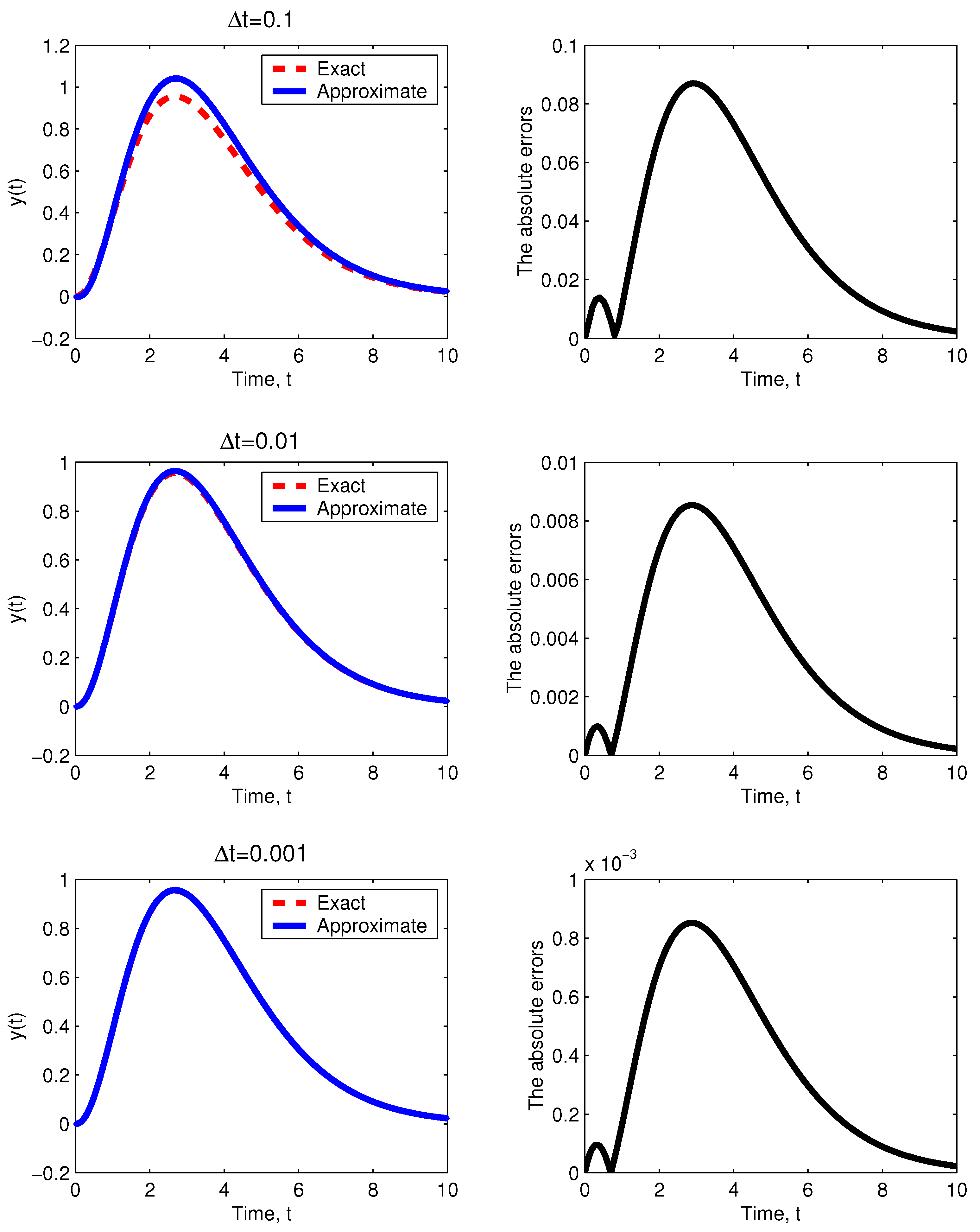
In this section, we establish the important formulas and properties for the new differential and integral operators.

For simplicity, we denoted ${\displaystyle {}^C{D}_{a,t,w,\delta }^{p,q,r,r}}$ by ${\mathcal{D}}_{a,w,\delta }^{p,q,r}$, and $I_{a,t,w,\delta }^{p,q,r}$ by ${\mathcal{I}}_{a,w,\delta }^{p,q,r}$.

Lemma 3.

The mixed fractional derivative ${\mathcal{D}}_{a,w,\delta }^{p,q,r}$ could be expressed as follows:

$${\mathcal{D}}_{a,w,\delta }^{p,q,r}u\left(t\right)=\frac{H(p+q-1)}{2-p-q}\sum _{k=0}^{+\infty }{(-\delta {\mu }_{p,q})}^k{}^{RL}{\mathcal{I}}_{a,w}^{kr+q}\left(\frac{{\left(wu\right)}^{\prime }}{w}\right)\left(t\right).$$

(16)

Proof. 

Since the Mittag–Leffler function $E_{p,q}\left(t\right)$ was the entire function of t, then ${\mathcal{D}}_{a,w,\delta }^{p,q,r}$ could be expressed as follows:

$$\begin{array}{ccc}\hfill {\mathcal{D}}_{a,w,\delta }^{p,q,r}u\left(t\right)& =& \frac{H(p+q-1)}{2-p-q}\frac{1}{w\left(t\right)}\sum _{k=0}^{+\infty }\frac{{(-\delta {\mu }_{p,q})}^k}{\mathsf{\Gamma }(rk+q)}{\int }_a^t{(t-\tau )}^{rk+q-1}{\left(wu\right)}^{\prime }\left(\tau \right)d\tau \hfill \\ & =& \frac{H(p+q-1)}{2-p-q}\sum _{k=0}^{+\infty }{(-\delta {\mu }_{p,q})}^k\frac{1}{\mathsf{\Gamma }(rk+q)}\frac{1}{w\left(t\right)}{\int }_a^t{(t-\tau )}^{rk+q-1}{\left(wu\right)}^{\prime }\left(\tau \right)d\tau \hfill \\ & =& \frac{H(p+q-1)}{2-p-q}\sum _{k=0}^{+\infty }{(-\delta {\mu }_{p,q})}^k{}^{RL}{\mathcal{I}}_{a,w}^{kr+q}\left(\frac{{\left(wu\right)}^{\prime }}{w}\right)\left(t\right).\hfill \end{array}$$

This completes the proof. □

Remark 3.

Lemma 3 extended the recent results established by Zitane and Torres in Lemma 3 of [18].

Theorem 3.

Let $(p,q)\in {[0,1]}^2$, $r>0$, $\delta \in {\mathbb{R}}^{\ast }$ and $u\in H^1(a,b)$. Then we have the following property:

$${\mathcal{I}}_{a,w,\delta }^{p,q,r}\left({\mathcal{D}}_{a,w,\delta }^{p,q,r}u\right)\left(t\right)=u\left(t\right)-\frac{w\left(a\right)u\left(a\right)}{w\left(t\right)}.$$

(17)

Proof. 

When $q\ne 1$, we had the following:

$${\displaystyle {\mathcal{I}}_{a,w,\delta }^{p,q,r}\left({\mathcal{D}}_{a,w,\delta }^{p,q,r}u\right)\left(t\right)=\frac{2-p-q}{H(p+q-1)}\left[{}^{RL}{\mathcal{I}}_{a,w}^{1-q}\left({\mathcal{D}}_{a,w,\delta }^{p,q,r}u\right)\left(t\right)+\delta {\mu }_{p,q}{}^{RL}{\mathcal{I}}_{a,w}^{1+r-q}\left({\mathcal{D}}_{a,w,\delta }^{p,q,r}u\right)\left(t\right)\right].}$$

By applying Lemma 3, we obtained the following:

$$\begin{array}{ccc}\hfill {\mathcal{I}}_{a,w,\delta }^{p,q,r}\left({\mathcal{D}}_{a,w,\delta }^{p,q,r}u\right)\left(t\right)& =& {\displaystyle {}^{RL}{\mathcal{I}}_{a,w}^{1-q}\left[\sum _{k=0}^{+\infty }{(-\delta {\mu }_{p,q})}^k{}^{RL}{\mathcal{I}}_{a,w}^{kr+q}\left(\frac{{\left(wu\right)}^{\prime }}{w}\right)\left(t\right)\right]}\hfill \\ & & {\displaystyle +\delta {\mu }_{p,q}{}^{RL}{\mathcal{I}}_{a,w}^{1+r-q}\left[\sum _{k=0}^{+\infty }{(-\delta {\mu }_{p,q})}^k{}^{RL}{\mathcal{I}}_{a,w}^{kr+q}\left(\frac{{\left(wu\right)}^{\prime }}{w}\right)\left(t\right)\right]}\hfill \\ & =& \sum _{k=0}^{+\infty }{(-\delta {\mu }_{p,q})}^k{}^{RL}{\mathcal{I}}_{a,w}^{kr+1}\left(\frac{{\left(wu\right)}^{\prime }}{w}\right)\left(t\right)-\sum _{k=1}^{+\infty }{(-\delta {\mu }_{p,q})}^k{}^{RL}{\mathcal{I}}_{a,w}^{kr+1}\left(\frac{{\left(wu\right)}^{\prime }}{w}\right)\left(t\right)\hfill \\ & =& {}^{RL}{\mathcal{I}}_{a,w}^1\left(\frac{{\left(wu\right)}^{\prime }}{w}\right)\left(t\right)\hfill \\ & =& \frac{1}{w\left(t\right)}{\int }_a^t{\left(wu\right)}^{\prime }\left(\tau \right)d\tau =u\left(t\right)-\frac{w\left(a\right)u\left(a\right)}{w\left(t\right)}.\hfill \end{array}$$

For $q=1$, we had the following:

$$\begin{array}{ccc}\hfill {\mathcal{I}}_{a,w,\delta }^{p,1,r}\left({\mathcal{D}}_{a,w,\delta }^{p,1,r}u\right)\left(t\right)& =& {\displaystyle \frac{1-p}{H\left(p\right)}({\mathcal{D}}_{a,w,\delta }^{p,q,r}u)\left(t\right)+\frac{\delta p}{H\left(p\right)}{}^{RL}{\mathcal{I}}_{a,w}^r\left({\mathcal{D}}_{a,w,\delta }^{p,q,r}u\right)\left(t\right)}\hfill \\ & =& \sum _{k=0}^{+\infty }{(-\delta {\mu }_{p,1})}^k{}^{RL}{\mathcal{I}}_{a,w}^{kr+1}\left(\frac{{\left(wu\right)}^{\prime }}{w}\right)\left(t\right)\hfill \\ & & {\displaystyle +\delta {\mu }_{p,1}{}^{RL}{\mathcal{I}}_{a,w}^r\left[\sum _{k=0}^{+\infty }{(-\delta {\mu }_{p,1})}^k{}^{RL}{\mathcal{I}}_{a,w}^{kr+1}\left(\frac{{\left(wu\right)}^{\prime }}{w}\right)\left(t\right)\right]}\hfill \\ & =& \sum _{k=0}^{+\infty }{(-\delta {\mu }_{p,1})}^k{}^{RL}{\mathcal{I}}_{a,w}^{kr+1}\left(\frac{{\left(wu\right)}^{\prime }}{w}\right)\left(t\right)-\sum _{k=1}^{+\infty }{(-\delta {\mu }_{p,1})}^k{}^{RL}{\mathcal{I}}_{a,w}^{kr+1}\left(\frac{{\left(wu\right)}^{\prime }}{w}\right)\left(t\right)\hfill \\ & =& {}^{RL}{\mathcal{I}}_{a,w}^1\left(\frac{{\left(wu\right)}^{\prime }}{w}\right)\left(t\right)\hfill \\ & =& u\left(t\right)-\frac{w\left(a\right)u\left(a\right)}{w\left(t\right)}.\hfill \end{array}$$

Hence, the proof was complete. □

It was obvious that when $w\left(t\right)=1$, we obtained the following first corollary of Theorem 3 that extended the Newton–Leibniz formula given in [20].

Corollary 1.

The new mixed fractional derivative and integral satisfied the Newton–Leibniz formula. In other words, we had the following:

$${\mathcal{I}}_{a,1,\delta }^{p,q,r}\left({\mathcal{D}}_{a,1,\delta }^{p,q,r}u\right)\left(t\right)=u\left(t\right)-u\left(a\right).$$

(18)

Clearly, ${\mathcal{D}}_{a,1,\delta }^{p,q,r}\left(c\right)=0$ for all constant function $u\left(t\right)=c$. Moreover, we found the following result.

Corollary 2.

Let u be a solution of the following fractional differential equation:

$${\mathcal{D}}_{a,1,\delta }^{p,q,r}u\left(t\right)=0.$$

(19)

Then the function u is a constant function.

Proof. 

It follows from (18) that $u\left(t\right)=u\left(a\right)$. This proves that u is a constant function. □

6. Numerical Scheme

In this section, we first developed a numerical method to approximate the solution of the following FDE with the new mixed fractional derivative, as given by the following:

$${\mathcal{D}}_{a,w,\delta }^{p,q,r}y\left(t\right)=f\left(t,y\left(t\right)\right),$$

(20)

where $t\in [a,b]$, $f:[a,b]\times \mathbb{R}\to \mathbb{R}$ is a continuous function and (20) is subject to the given initial condition

$$y\left(a\right)=y_0.$$

From Theorem 3, Equation (20) could be converted into the following fractional integral equation:

$$\begin{array}{c}\hfill y\left(t\right)-{\displaystyle \frac{y\left(a\right)w\left(a\right)}{w\left(t\right)}}={\mathcal{I}}_{a,w,\delta }^{p,q,r}f\left(t,y\left(t\right)\right).\end{array}$$

(21)

Therefore, we evaluated specific scenarios. When $q=1$, we had

$${\displaystyle y\left(t\right)-{\displaystyle \frac{y\left(a\right)w\left(a\right)}{w\left(t\right)}}=\frac{1-p}{H\left(p\right)}f\left(t,y\left(t\right)\right)+\frac{\delta p}{H\left(p\right)}{}^{RL}{\mathcal{I}}_{a,w}^{r}f\left(t,y\left(t\right)\right),}$$

which implied that

$$\begin{array}{c}\hfill y\left(t\right)={\displaystyle \frac{y\left(a\right)w\left(a\right)}{w\left(t\right)}}+{\displaystyle \frac{1-p}{H\left(p\right)}}f\left(t,y\left(t\right)\right)+{\displaystyle \frac{\delta p}{H\left(p\right)\mathsf{\Gamma }\left(r\right)}}{\displaystyle \frac{1}{w\left(t\right)}}{\int }_a^t{(t-\tau )}^{r-1}w\left(\tau \right)f\left(\tau ,y\left(\tau \right)\right)d\tau .\end{array}$$

(22)

Let $\Delta t$ be the discretization step and $t_n=a+n\Delta t$, with $n\in \mathrm{I}\mathrm{N}$. We had the following:

$$\begin{array}{ccc}\hfill y\left(t_{n+1}\right)& =& {\displaystyle \frac{y_{0}w\left(a\right)}{w\left(t_n\right)}}+{\displaystyle \frac{1-p}{H\left(p\right)}}f\left(t_n,y\left(t_n\right)\right)\hfill \\ & & +{\displaystyle \frac{\delta p}{H\left(p\right)\mathsf{\Gamma }\left(r\right)w\left(t_n\right)}}{\int }_a^{t_{n+1}}{(t_{n+1}-\tau )}^{r-1}w\left(\tau \right)f\left(\tau ,y\left(\tau \right)\right)d\tau .\hfill \end{array}$$

Then

$$\begin{array}{ccc}\hfill y\left(t_{n+1}\right)& =& {\displaystyle \frac{y_{0}w\left(a\right)}{w\left(t_n\right)}}+{\displaystyle \frac{1-p}{H\left(p\right)}}f\left(t_n,y\left(t_n\right)\right)\hfill \\ & & +{\displaystyle \frac{\delta p}{H\left(p\right)\mathsf{\Gamma }\left(r\right)w\left(t_n\right)}}\sum _{k=0}^n{\int }_{t_k}^{t_{k+1}}{(t_{n+1}-\tau )}^{r-1}g\left(\tau ,y\left(\tau \right)\right)d\tau ,\hfill \end{array}$$

(23)

where $g\left(\tau ,y\left(\tau \right)\right)=w\left(\tau \right)f\left(\tau ,y\left(\tau \right)\right)$. The function g could be approximated over $[t_k,t_{k+1}]$ by means of the Lagrange polynomial interpolation, as follows:

$$\begin{array}{ccc}\hfill P_k\left(\tau \right)& =& {\displaystyle \frac{\tau -t_k}{t_{k-1}-t_k}}g\left(t_{k-1},y\left(t_{k-1}\right)\right)+{\displaystyle \frac{\tau -t_{k-1}}{t_k-t_{k-1}}}g\left(t_k,y\left(t_k\right)\right),\hfill \\ & \simeq & {\displaystyle \frac{g(t_{k-1},y_{k-1})}{\Delta t}}(t_k-\tau )+{\displaystyle \frac{g(t_k,y_k)}{\Delta t}}(\tau -t_{k-1}).\hfill \end{array}$$

(24)

Hence,

$$\begin{array}{ccc}\hfill y\left(t_{n+1}\right)& =& {\displaystyle \frac{y_{0}w\left(0\right)}{w\left(t_n\right)}}+{\displaystyle \frac{1-p}{H\left(p\right)}}f\left(t_n,y_n\right)\hfill \\ & & +{\displaystyle \frac{\delta p}{H\left(p\right)\mathsf{\Gamma }\left(r\right)w\left(t_n\right)}}\sum _{k=0}^n[{\displaystyle \frac{g\left(t_k,y_k\right)}{\Delta t}}{\int }_{t_k}^{t_{k+1}}\left(\tau -t_{k-1}\right){\left(t_{n+1}-\tau \right)}^{r-1}d\tau \hfill \\ & & +{\displaystyle \frac{g\left(t_{k-1},x_{k-1}\right)}{\Delta t}}{\int }_{t_k}^{t_{k+1}}\left(t_k-\tau \right){\left(t_{n+1}-\tau \right)}^{r-1}d\tau ].\hfill \end{array}$$

Since

$$\begin{array}{ccc}\hfill {\int }_{t_k}^{t_{k+1}}{(t_{n+1}-\tau )}^{r-1}(\tau -t_{k-1})d\tau & =& {\displaystyle \frac{{(\Delta t)}^{r+1}}{r(r+1)}}[{(n-k+1)}^r(n-k+2+r)\hfill \\ & & -{(n-k)}^r(n-k+2+2r)],\hfill \end{array}$$

(25)

and

$$\begin{array}{ccc}\hfill {\int }_{t_k}^{t_{k+1}}{(t_{n+1}-\tau )}^{r-1}(t_k-\tau )d\tau & =& {\displaystyle \frac{{(\Delta t)}^{r+1}}{r(r+1)}}[{(n-k)}^r(n-k+1+r)\hfill \\ & & -{(n-k+1)}^{r+1}],\hfill \end{array}$$

(26)

we had the following numerical scheme for the case of $q=1$:

$$\begin{array}{ccc}\hfill y_{n+1}& =& {\displaystyle \frac{y_{0}w\left(0\right)}{w\left(t_n\right)}}+{\displaystyle \frac{1-p}{H\left(p\right)}}f\left(t_n,y_n\right)\hfill \\ \hfill & & +{\displaystyle \frac{\delta p{(\Delta t)}^r}{H\left(p\right)\mathsf{\Gamma }(r+2)w\left(t_n\right)}}\sum _{k=0}^n(w\left(t_k\right)f\left(t_k,y_k\right){\mathcal{A}}_{n,k}^r\hfill \\ & & +w\left(t_{k-1}\right)f\left(t_{k-1},y_{k-1}\right){\mathcal{B}}_{n,k}^r),\hfill \end{array}$$

(27)

where

$$\begin{array}{ccc}\hfill {\mathcal{A}}_{n,k}^r& =& {(n-k+1)}^r(n-k+2+r)-{(n-k)}^r(n-k+2+2r),\hfill \\ \hfill {\mathcal{B}}_{n,k}^r& =& {(n-k)}^r(n-k+1+r)-{(n-k+1)}^{r+1}.\hfill \end{array}$$

Remark 4.

The numerical scheme given in (27) accounted for the numerical method of Hattaf et al. [16], when $q=\delta =1$; Toufik and Atangana [17], when $w\left(t\right)=1$, $q=\delta =1$, and $r=p$; and the recent numerical scheme presented in [18], when $q=1$ and $\delta =ln\left(\overline{p}\right)$, with $\overline{p}>0$.

For $q\ne 1$, Equation (21) became:

$$\begin{array}{ccc}\hfill y\left(t\right)& =& {\displaystyle \frac{y\left(a\right)w\left(a\right)}{w\left(t\right)}}+{\displaystyle \frac{2-p-q}{H(p+q-1)w\left(t\right)}}[{\displaystyle \frac{1}{\mathsf{\Gamma }(1-q)}}{\int }_a^t{(t-\tau )}^{-q}w\left(\tau \right)f\left(\tau ,y\left(\tau \right)\right)d\tau \hfill \\ & & +{\displaystyle \frac{\delta {\mu }_{p,q}}{\mathsf{\Gamma }(r-q+1)}}{\int }_a^t{(t-\tau )}^{r-q}w\left(\tau \right)f\left(\tau ,y\left(\tau \right)\right)d\tau ].\hfill \end{array}$$

Thus,

$$\begin{array}{ccc}\hfill y\left(t_{n+1}\right)& =& {\displaystyle \frac{y\left(a\right)w\left(a\right)}{w\left(t_n\right)}}+{\displaystyle \frac{2-p-q}{H(p+q-1)w\left(t_n\right)}}[{\displaystyle \frac{1}{\mathsf{\Gamma }(1-q)}}\sum _{k=0}^n{\int }_{t_k}^{t_{k+1}}{(t_{n+1}-\tau )}^{-q}g\left(\tau ,y\left(\tau \right)\right)d\tau \hfill \\ & & +{\displaystyle \frac{\delta {\mu }_{p,q}}{\mathsf{\Gamma }(r-q+1)}}\sum _{k=0}^n{\int }_{t_k}^{t_{k+1}}{(t_{n+1}-\tau )}^{r-q}g\left(\tau ,y\left(\tau \right)\right)d\tau ].\hfill \end{array}$$

Similarly, we obtained the following scheme for the case of $q\ne 1$:

$$\begin{array}{ccc}\hfill y_{n+1}& =& {\displaystyle \frac{y_{0}w\left(a\right)}{w\left(t_n\right)}}+{\displaystyle \frac{(2-p-q){(\Delta t)}^{1-q}}{H(p+q-1)w\left(t_n\right)}}[{\displaystyle \frac{1}{\mathsf{\Gamma }(3-q)}}\sum _{k=0}^n(w\left(t_k\right)f\left(t_k,y_k\right){\mathcal{A}}_{n,k}^r\hfill \\ \hfill & & +w\left(t_{k-1}\right)f\left(t_{k-1},y_{k-1}\right){\mathcal{B}}_{n,k}^r)+{\displaystyle \frac{\delta {\mu }_{p,q}{(\Delta t)}^r}{\mathsf{\Gamma }(r-q+3)}}\sum _{k=0}^n(w\left(t_k\right)f\left(t_k,y_k\right){\mathcal{A}}_{n,k}^{r-q+1}\hfill \\ & & +w\left(t_{k-1}\right)f\left(t_{k-1},y_{k-1}\right){\mathcal{B}}_{n,k}^{r-q+1}\left)\right].\hfill \end{array}$$

(28)

Now, we investigated the numerical error of our proposed approximation scheme by assuming that $g=wf$ had a bounded second derivative. For the case of $q=1$, we found the following:

$$\begin{array}{ccc}\hfill y\left(t_{n+1}\right)& =& {\displaystyle \frac{y_{0}w\left(a\right)}{w\left(t_n\right)}}+{\displaystyle \frac{1-p}{H\left(p\right)}}f\left(t_n,y\left(t_n\right)\right)\hfill \\ & & +{\displaystyle \frac{\delta p}{H\left(p\right)\mathsf{\Gamma }\left(r\right)w\left(t_n\right)}}\sum _{k=0}^n{\int }_{t_k}^{t_{k+1}}{(t_{n+1}-\tau )}^{r-1}g\left(\tau ,y\left(\tau \right)\right)d\tau .\hfill \end{array}$$

Hence,

$$\begin{array}{ccc}\hfill y\left(t_{n+1}\right)& =& {\displaystyle \frac{y_{0}w\left(a\right)}{w\left(t_n\right)}}+{\displaystyle \frac{1-p}{H\left(p\right)}}f\left(t_n,y\left(t_n\right)\right)+\frac{p\delta }{H\left(p\right)\mathsf{\Gamma }\left(r\right)w\left(t_n\right)}\sum _{k=0}^n{\int }_{t_k}^{t_{k+1}}(P_k\left(\tau \right)\hfill \\ & & +\frac{(\tau -t_k)(\tau -t_{k-1})}{2!}{g}^{\left(2\right)}\left({\xi }_{\tau },y\left({\xi }_{\tau }\right)\right)){(t_{n+1}-\tau )}^{r-1}d\tau \hfill \\ & =& {\displaystyle \frac{y_{0}w\left(a\right)}{w\left(t_n\right)}}+{\displaystyle \frac{1-\alpha }{H\left(p\right)}}f\left(t_n,y\left(t_n\right)\right)\hfill \\ & & +{\displaystyle \frac{p\delta {(\Delta t)}^r}{H\left(p\right)\mathsf{\Gamma }(r+2)w\left(t_n\right)}}\sum _{k=0}^n\left(g\left(t_k,y_k\right){\mathcal{A}}_{n,k}^r+g\left(t_{k-1},y_{k-1}\right){\mathcal{B}}_{n,k}^r\right)+{\mathcal{R}}_n^{p,1,\delta },\hfill \end{array}$$

where the approximation error ${\mathcal{R}}_n^{p,1,\delta }$ was given by the following:

$${\mathcal{R}}_n^{p,1,\delta }={\displaystyle \frac{p\delta }{H\left(p\right)\mathsf{\Gamma }\left(r\right)w\left(t_n\right)}}\sum _{k=0}^n{\int }_{t_k}^{t_{k+1}}\frac{(\tau -t_k)(\tau -t_{k-1})}{2!}{g}^{\left(2\right)}\left({\xi }_{\tau },y\left({\xi }_{\tau }\right)\right){(t_{n+1}-\tau )}^{r-1}d\tau .$$

(29)

As the function $\tau \mapsto (\tau -t_{k-1}){(t_{n+1}-\tau )}^{r-1}$ was positive on $[t_k,t_{k+1}]$, then there existed a ${\xi }_k\in [t_k,t_{k+1}]$, such that:

$$\begin{array}{ccc}\hfill {\mathcal{R}}_n^{p,1,\delta }& =& {\displaystyle \frac{p\delta }{H\left(p\right)\mathsf{\Gamma }\left(r\right)w\left(t_n\right)}}\sum _{k=0}^n{g}^{\left(2\right)}\left({\xi }_k,y\left({\xi }_k\right)\right)\frac{({\xi }_k-t_k)}{2}{\int }_{t_k}^{t_{k+1}}(\tau -t_{k-1}){(t_{n+1}-\tau )}^{r-1}d\tau \hfill \\ & =& {\displaystyle \frac{p\delta {(\Delta t)}^{r+1}}{2H\left(p\right)\mathsf{\Gamma }(r+2)w\left(t_n\right)}}\sum _{k=0}^n{g}^{\left(2\right)}\left({\xi }_k,y\left({\xi }_k\right)\right)({\xi }_k-t_k){\mathcal{A}}_{n,k}^r.\hfill \end{array}$$

Thus,

$$\begin{array}{ccc}\hfill \left|{\mathcal{R}}_n^{p,1,\delta }\right|& \le & {\displaystyle \frac{p\delta {(\Delta t)}^{r+2}}{2H\left(p\right)\mathsf{\Gamma }(r+2)w\left(t_n\right)}}\underset{\tau \in [a,t_{n+1}]}{max}\left|g^{\left(2\right)}(\tau ,y\left(\tau \right))\right|\left|\sum _{k=0}^n{\mathcal{A}}_{n,k}^r\right|.\hfill \end{array}$$

Based on the following formulas

$$\begin{array}{ccc}\hfill {\mathcal{A}}_{n,k}^r& \le & (n-k+2+r)\left[{(n+1)}^r-r{n}^r\right],\hfill \\ \hfill \sum _{k=0}^n(n-k+2+r)& =& \frac{(n+1)(n+4+2r)}{2},\hfill \end{array}$$

we found the following:

$$\left|{\mathcal{R}}_n^{p,1,\delta }\right|\le \frac{p\delta {(\Delta t)}^{r+2}(n+1)(n+4+2r)[{(n+1)}^r-r{n}^r]}{4H\left(p\right)\mathsf{\Gamma }(r+2)w\left(t_n\right)}\underset{\tau \in [a,t_{n+1}]}{max}\left|g^{\left(2\right)}(\tau ,y\left(\tau \right))\right|.$$

(30)

In the same way as above, it was not hard to establish the approximation error for the case of $q\ne 1$.

To illustrate our numerical scheme, we considered the following FDE with a mixed fractional derivative:

$$\left\{\begin{array}{c}{\mathcal{D}}_{a,w,\delta }^{p,1,r}y\left(t\right)=t^2{e}^{-t},\hfill \\ y\left(0\right)=0.\hfill \end{array}\right.$$

(31)

Let $w\left(t\right)=e^t$. By applying the fractional integral to both sides of (31) and using Theorem 3, we obtained the exact solution of (31), which was given by the following:

$$y\left(t\right)=\left({\displaystyle \frac{1-p}{H\left(p\right)}}+{\displaystyle \frac{2p\delta t^r}{H\left(p\right)\mathsf{\Gamma }(r+3)}}\right)t^2{e}^{-t}.$$

(32)

Now, we applied the developed numerical scheme for the case of $q=1$, as presented in (27), to approximate the solution of (31). For all numerical simulations, we chose the normalization function, as follows:

$$H\left(p\right)=1-p+{\displaystyle \frac{p}{\mathsf{\Gamma }\left(p\right)}}.$$

(33)

The comparison between the exact and approximate solutions of (31), with the corresponding absolute errors, is shown in Figure 1 for the different values of $\Delta t$, $p=0.7$, $r=0.8$, and $\delta =2.5$. In addition,

Table 1. The maximum errors corresponding to different values of $\Delta t$, with $p=0.7$, $r=0.8$, and $\delta =2.5$.

Discretization Step ($\mathbf{\Delta }\mathit{t}$)	Error
0.1	$8.6991\times {10}^{-2}$
0.01	$8.5373\times {10}^{-3}$
0.001	$8.5204\times {10}^{-4}$

presents the maximum errors for numerous values of $\Delta t$.

From Figure 1, we observed that the developed numerical scheme had very good agreement between the exact and approximate solutions for the different values of the discretization step $\Delta t$. Furthermore, Table 1 shows that the convergence of the numerical approximation depended on the discretization step $\Delta t$. By comparing the exact and approximate solutions, we deduced that the new developed numerical scheme was effective and rapidly converged to the exact solution.

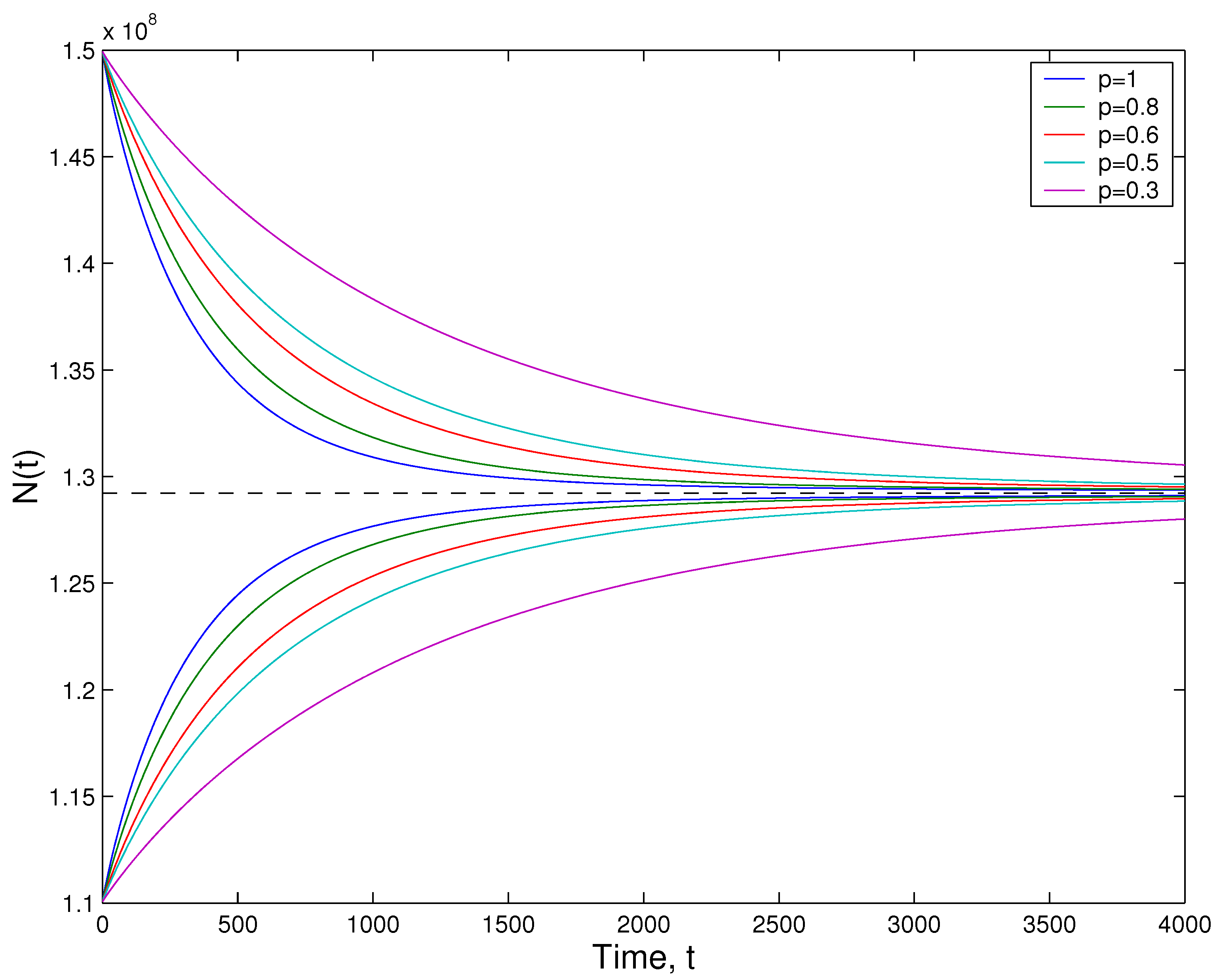
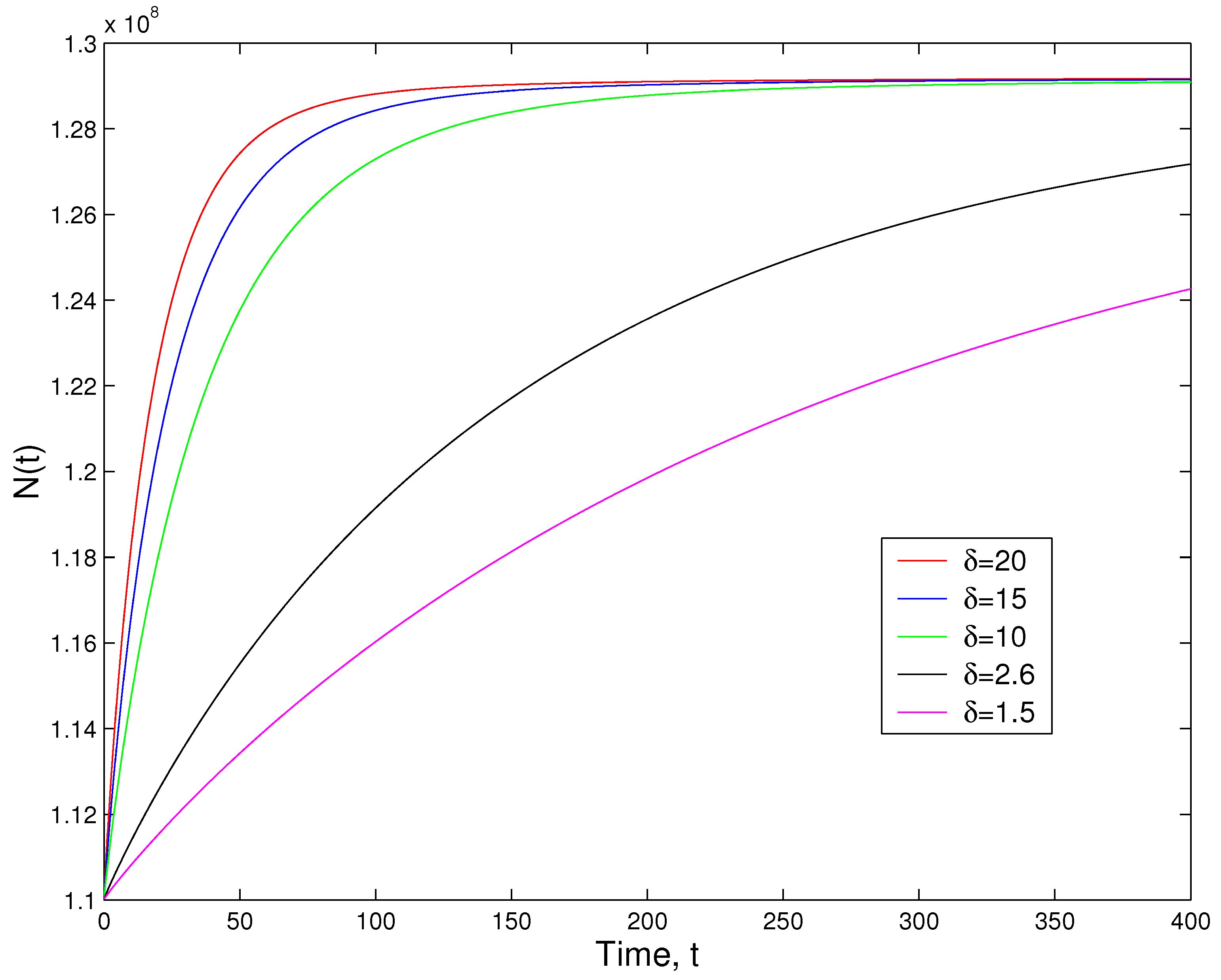
7. Application in Computational Biology

Computational biology is a branch of biology that uses mathematical modeling and computational simulations in order to understand biological systems and relationships. Therefore, we considered the following FDE system that described the evolution of a cell population in the human body:

$${\mathcal{D}}_{0,w,\delta }^{p,1,r}N\left(t\right)=\lambda -dN\left(t\right),$$

(34)

where $N\left(t\right)$ is the total cell population produced at rate $\lambda$ and dying naturally at rate d. Furthermore, the new fractional derivative used in (34) enabled us to investigate the dynamical behavior of a cell population with a large variety of parameters that could account for natural constraints and the multitude of factors influencing cell growth in the human body, such as nutrition, genetics, environment, stress, competition between cells, etc.

By applying the Laplace transform to (34), we obtained the following:

$$\mathcal{L}\left\{w\left(t\right){\mathcal{D}}_{0,w,\delta }^{p,1,r}N\left(t\right)\right\}=\lambda \mathcal{L}\left\{w\left(t\right)\right\}-d\mathcal{L}\left\{w\left(t\right)N\left(t\right)\right\}.$$

According Theorem 2, we had the following:

$$\mathcal{L}\left\{w\left(t\right)N\left(t\right)\right\}\left(s\right)=\frac{H\left(p\right)w\left(0\right)N\left(0\right)s^{r-1}}{[H\left(p\right)+d(1-p)]s^r+dp\delta }+\frac{\lambda (1-p)s^{\beta }+p\lambda \delta }{[N\left(p\right)+d(1-p)]s^r+dp\delta }\mathcal{L}\left\{w\left(t\right)\right\}\left(s\right).$$

Then,

$$\mathcal{L}\left\{w\left(t\right)N\left(t\right)\right\}\left(s\right)=\frac{H\left(p\right)w\left(0\right)N\left(0\right)s^{r-1}}{a_p{s}^r+dp\delta }+\frac{\lambda (1-p)s^{\beta }+p\lambda \delta }{a_p{s}^r+dp\delta }\mathcal{L}\left\{w\left(t\right)\right\}\left(s\right),$$

where $a_p=H\left(p\right)+d(1-p)$. Hence,

$$\begin{array}{ccc}\hfill \mathcal{L}\left\{w\right(t\left)N\right(t\left)\right\}\left(s\right)& =& \frac{H\left(p\right)w\left(0\right)N\left(0\right)}{a_p}\frac{s^{r-1}}{s^r+\frac{dp\delta }{a_p}}+\frac{\lambda (1-p)}{a_p}\frac{s^{r-1}}{s^r+\frac{dp\delta }{a_{\alpha }}}s\mathcal{L}\left\{w\left(t\right)\right\}\left(s\right)\hfill \\ & & +\frac{p\lambda \delta }{a_p}\frac{1}{s^r+\frac{dp\delta }{a_p}}\mathcal{L}\left\{w\left(t\right)\right\}\left(s\right)\hfill \\ & =& \frac{H\left(p\right)w\left(0\right)N\left(0\right)}{a_p}\mathcal{L}\left\{E_r\left(-\frac{dp\delta }{a_p}{t}^r\right)\right\}\hfill \\ & & +\frac{\lambda (1-p)}{a_p}\mathcal{L}\left\{E_r\left(-\frac{dp\delta }{a_p}{t}^r\right)\right\}\left(\mathcal{L}\left\{w^{\prime }\left(t\right)\right\}+w\left(0\right)\right)\hfill \\ & & -\frac{\lambda }{d}\mathcal{L}\left\{\frac{d}{dt}{E}_r\left(-\frac{dp\delta }{a_p}{t}^r\right)\right\}\mathcal{L}\left\{w\left(t\right)\right\}.\hfill \end{array}$$

Thus,

$$\begin{array}{ccc}\hfill w\left(t\right)N\left(t\right)& =& \frac{H\left(p\right)w\left(0\right)N\left(0\right)}{a_p}{E}_r\left(-\frac{dp\delta }{a_p}{t}^r\right)+\frac{\lambda (1-p)}{a_p}{E}_r\left(-\frac{dp\delta }{a_p}{t}^r\right)\ast w^{\prime }\left(t\right)\hfill \\ & & +\frac{\lambda (1-p)w\left(0\right)}{a_p}{E}_r\left(-\frac{dp\delta }{a_p}{t}^r\right)-\frac{\lambda }{d}\frac{d}{dt}{E}_r\left(-\frac{dp\delta }{a_p}{t}^r\right)\ast w\left(t\right).\hfill \end{array}$$

However, we had the following:

$$\frac{d}{dt}{E}_r\left(-\frac{dp\delta }{a_p}{t}^r\right)\ast w\left(t\right)=E_r\left(-\frac{dp\delta }{a_p}{t}^r\right)w\left(0\right)-w\left(t\right)+E_r\left(-\frac{dp\delta }{a_p}{t}^r\right)\ast w^{\prime }\left(t\right).$$

This led to the following:

$$N\left(t\right)=\frac{\lambda }{d}+\frac{H\left(p\right)w\left(0\right)}{a_{p}w\left(t\right)}\left(N\left(0\right)-\frac{\lambda }{d}\right)E_r\left(-\frac{dp\delta }{a_p}{t}^r\right)-\frac{\lambda H\left(p\right)}{d{a}_{p}w\left(t\right)}{E}_r\left(-\frac{dp\delta }{a_p}{t}^r\right)\ast w^{\prime }\left(t\right).$$

(35)

When the weight function was constant, Equation (35) became:

$$N\left(t\right)=\frac{\lambda }{d}+\frac{H\left(p\right)w\left(0\right)}{a_{p}w\left(t\right)}\left(N\left(0\right)-\frac{\lambda }{d}\right)E_r\left(-\frac{dp\delta }{a_p}{t}^r\right).$$

(36)

For liver cells, also called hepatocytes, $\lambda =5.04\pm 0.71\times {10}^5$ cell/mL/day and $d=0.0039$ day${}^{-1}$ [21]. Figure 2 shows the impact of order p on the dynamical behavior of the solutions of (34), with two initial conditions, $N\left(0\right)=1.1\times {10}^8$ and $N\left(0\right)=1.5\times {10}^8$ cells/mL, for $\delta =1$ and $r=0.95$.

Next, we investigated the impact of the parameter p on the dynamics of (34), with $p=0.8$ and $r=0.95$. Figure 3 shows the results.

8. Conclusions

This study introduced a new mixed fractional derivative in the sense of Caputo and Riemann–Liouville, which covered many definitions of fractional derivatives, both with singular and non-singular kernels, including the Riemann–Liouville fractional derivative [1,2]; the Caputo fractional derivative [3]; the CF fractional derivative [4]; the AB fractional derivative [5]; the weighted-AB fractional derivative [6]; the power fractional derivative [13]; the fractional derivative with the Mittag–Leffler kernel of two parameters [14]; and also the GHF derivative [7]. Furthermore, the fractional integral operator associated with the new mixed fractional derivative was defined to include the many well-known forms of fractional integrals recorded in the fractional calculus literature. In addition, the fundamental properties of the fractional operators of differentiation and integration were investigated. We developed an explicit numerical method based on the Lagrange polynomial interpolation for finding an approximate solution of differential equations with mixed fractional derivatives. Our method improved and generalized the recent numerical methods presented in [16,17,18]. Our results were then effectively applied to a biological system that described the evolution of a cell population in the human body.

The key advantages of the new mixed fractional derivative operator include its non-locality and its flexibility. It could accommodate a wide range of parameters in order to better fit real data and more accurately model real-world problems. Additionally, the new mixed fractional derivative had a kernel with various parameters that included exponential, power-law, and Mittag–Leffler kernels. Based on the results and advantages, the development of a theory with a general derivative, as well as the derivation of a new version of fractal-fractional operators that can model complex behavior and processes in real-world phenomena, such as in [22,23,24], will be considered in future research.

References

1. Kilbas, A.A.; Srivastava, H.M.; Trujillo, J.J. Theory and Applications of Fractional Differential Equations; North-Holland Mathematics Studies; Elsevier: Amsterdam, The Netherlands, 2006. [Google Scholar]
2. Podlubny, I. Fractional Differential Equations; Academic Press: San Diego, CA, USA, 1999. [Google Scholar]
3. Caputo, M. Linear models of dissipation whose Q is almost frequency independent-II. Geophys. J. Int. 1967, 13, 529–539. [Google Scholar] [CrossRef]
4. Caputo, M.; Fabrizio, M. A new definition of fractional derivative without singular kernel. Prog. Fract. Differ. Appl. 2015, 1, 73–85. [Google Scholar]
5. Atangana, A.; Baleanu, D. New fractional derivatives with non-local and non-singular kernel: Theory and application to heat transfer model. Therm. Sci. 2016, 20, 763–769. [Google Scholar] [CrossRef]
6. Al-Refai, M. On weighted Atangana-Baleanu fractional operators. Adv. Differ. Equ. 2020, 2020, 3. [Google Scholar] [CrossRef]
7. Hattaf, K. A new generalized definition of fractional derivative with non-singular kernel. Computation 2020, 8, 49. [Google Scholar] [CrossRef]
8. Hattaf, K. A new class of generalized fractal and fractal-fractional derivatives with non-singular kernels. Fractal Fract. 2023, 7, 395. [Google Scholar] [CrossRef]
9. Chen, W. Time-space fabric underlying anomalous diffusion. Chaos Solitons Fractals 2006, 28, 923–929. [Google Scholar] [CrossRef]
10. Asma, M.Y.; Afzaal, M.; DarAssi, M.H.; Khan, M.A.; Alshahrani, M.Y.; Suliman, M. A mathematical model of vaccinations using new fractional order derivative. Vaccines 2022, 10, 1980. [Google Scholar] [CrossRef]
11. Cheneke, K.R.; Rao, K.P.; Edesssa, G.K. A new generalized fractional-order derivative and bifurcation analysis of cholera and human immunodeficiency co-infection dynamic transmission. Int. J. Math. Math. Sci. 2022, 2022, 7965145. [Google Scholar] [CrossRef]
12. Lemnaouar, M.R.; Taftaf, C.; Louartassi, C.Y. On the controllability of fractional semilinear systems via the generalized Hattaf fractional derivative. Int. J. Dyn. Control 2023, 1–8. [Google Scholar] [CrossRef]
13. Lotfi, E.M.; Zine, H.; Torres, D.F.M.; Yousfi, N. The power fractional calculus: First definitions and properties with applications to power fractional differential equations. Mathematics 2022, 10, 3594. [Google Scholar] [CrossRef]
14. Chinchole, S.M.; Bhadane, A.P. A new definition of fractional derivatives with Mittag–Leffler kernel of two parameters. Commun. Math. Appl. 2022, 13, 19–26. [Google Scholar] [CrossRef]
15. Hattaf, K. On the Stability and Numerical Scheme of Fractional Differential Equations with Application to Biology. Computation 2022, 10, 97. [Google Scholar] [CrossRef]
16. Hattaf, K.; Hajhouji, Z.; Ichou, M.A.; Yousfi, N. A Numerical Method for Fractional Differential Equations with New Generalized Hattaf Fractional Derivative. Math. Probl. Eng. 2022, 2022, 3358071. [Google Scholar] [CrossRef]
17. Toufik, M.; Atangana, A. New numerical approximation of fractional derivative with non-local and non-singular kernel: Application to chaotic models. Eur. Phys. J. Plus 2017, 132, 444. [Google Scholar] [CrossRef]
18. Zitane, H.; Torres, D.F.M. A class of fractional differential equations via power non-local and non-singular kernels: Existence, uniqueness and numerical approximations. Phys. D Nonlinear Phenom. 2024, 457, 133951. [Google Scholar] [CrossRef]
19. Wiman, A. Über den fundamental satz in der theorie der funktionen Ea(x). Acta Math. 1905, 29, 191–201. [Google Scholar] [CrossRef]
20. Baleanu, D.; Fernandez, A. On some new properties of fractional derivatives with Mittag–Leffler kernel. Commun. Nonlinear Sci. Numer. Simul. 2018, 59, 444–462. [Google Scholar] [CrossRef]
21. Eikenberry, S.; Hews, S.; Nagy, J.D.; Kuang, Y. The dynamics of a delay model of HBV infection with logistic hepatocyte growth. Math. Biosci. Eng. 2009, 6, 283–299. [Google Scholar]
22. Zhou, J.C.; Salahshour, S.; Ahmadian, A.; Senu, N. Modeling the dynamics of COVID-19 using fractal-fractional operator with a case study. Results Phys. 2022, 33, 105103. [Google Scholar] [CrossRef]
23. Hendy, M.H.; Amin, M.M.; Ezzat, M.A. Two-dimensional problem for thermoviscoelastic materials with fractional order heat transfer. J. Therm. Stress. 2019, 42, 1298–1315. [Google Scholar] [CrossRef]
24. Shymanskyi, V.; Sokolovskyy, I.; Sokolovskyy, Y.; Bubnyak, T. Variational Method for Solving the Time-Fractal Heat Conduction Problem in the Claydite-Block Construction. In Proceedings of the International Conference on Computer Science, Engineering and Education Applications, Kyiv, Ukraine, 21–22 February 2022; Springer: Berlin/Heidelberg, Germany, 2022; pp. 97–106. [Google Scholar]
Figure 1. The exact and numerical solutions of (31), with the corresponding absolute errors, for different values of Δ t .
Computation 12 00007 g001
Figure 2. The solution of (34) with two initial conditions for δ = 1 , r = 0.95 , and different values of p.
Computation 12 00007 g002
Figure 3. The impact of parameter δ on the dynamics of (34), with p = 0.8 and r = 0.95 .
Computation 12 00007 g003