
Performance and Application Analysis of a New Optimization Algorithm


Abstract
:1. Introduction
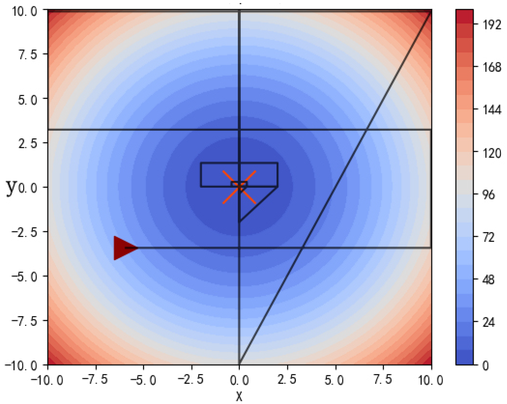
2. Studied System
- Line 3 writes Formula (1) as a computer program;
- Line 4 sets a loop body. The number of loops is determined by MSRALoop.
- Line 5 writes Formula (2) as a computer program.
- In line 6, the coordinate points scanned in the X direction are substituted into the test function to calculate and take the optimal value. For Project 1, this step is to collect the mutual inductance data scanned in the X direction and obtain the optimal value.
- In line 7, the Y coordinate corresponding to the best fitness is assigned to Yt as the initial value of the Y-direction scan.
- Line 8 writes Formula (6) as a computer program.
- In line 9, the coordinate points scanned in the Y direction are substituted into the test function to calculate and take the optimal value. For Project 1, this step collects the mutual inductance data scanned in the Y direction and obtains the optimal value.
- In line 11, judge whether the loop calculation is completed or not.
- In line 12, take the optimal value and the corresponding XY coordinates.
| Algorithm 1 The pseudo-code of the MSRA. | |
| 1 | Begin |
| 2 | Define the parameters: UB, LB, step, rows, Ysep, Ystep, Mter |
| 3 | Initialize the random position of search and rescue aircraft: X0. |
| 4 | While t in [1, MSRALoop] { |
| 5 | For i in range (0, step): { } End for |
| 6 | Calculate the fitness of all and then, obtain the best fitness of |
| 7 | Assign the Y coordinate corresponding to the best fitness to Yt |
| 8 | For i in range (0, step):{ } End for |
| 9 | Calculate the fitness of all , and then, obtain the best fitness of |
| 10 | Calculate the new UB, LB, and then, update UB, LB |
| 11 | t = t + 1} End While |
| 12 | Return bestFitness and the corresponding XY coordinates |
| 13 | End |
3. Performance of the Optimization Algorithm
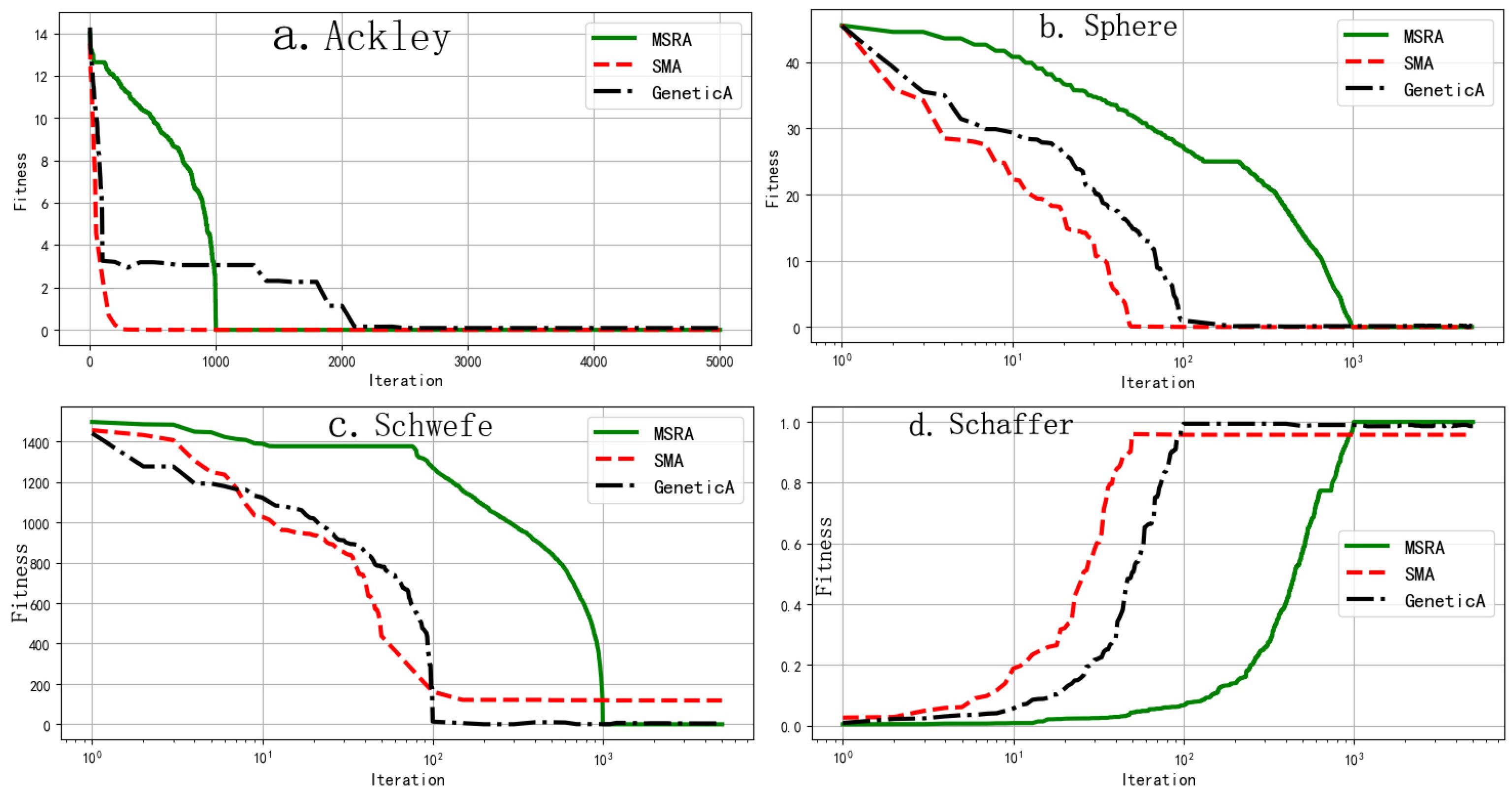
3.1. Ackley Function
3.2. Sphere Function
3.3. Schwefe Function
3.4. Schaffer Function
3.5. Performance Comparison between MSRA and Two Other Algorithms
4. Experiment
5. Result
6. Conclusions
Author Contributions
Funding
Acknowledgments
Conflicts of Interest
References
- Zheng, J.; Jettanasen, C. Analysis Of Mutual Inductance Between Transmitter And Receiver Coils In Wireless Power Transfer System Of Electric Vehicle. Adv. Electr. Electron. Eng. 2023, 21. [Google Scholar] [CrossRef]
- Xu, P.; Fu, C.; Li, J.-J.; Dong, L.; Zhao, S.-P. The research of estimating the location of radioactive sources using the Bayesian estimation. Nucl. Instruments Methods Phys. Res. Sect. Accel. Spectrometers Detect. Assoc. Equip. 2021, 1006, 165405. [Google Scholar] [CrossRef]
- Ma, D.; Mao, W.; Tan, W.; Gao, J.; Zhang, Z.; Xie, Y. Emission source tracing based on bionic algorithm mobile sensors with artificial olfactory system. Robotica 2022, 40, 976–996. [Google Scholar] [CrossRef]
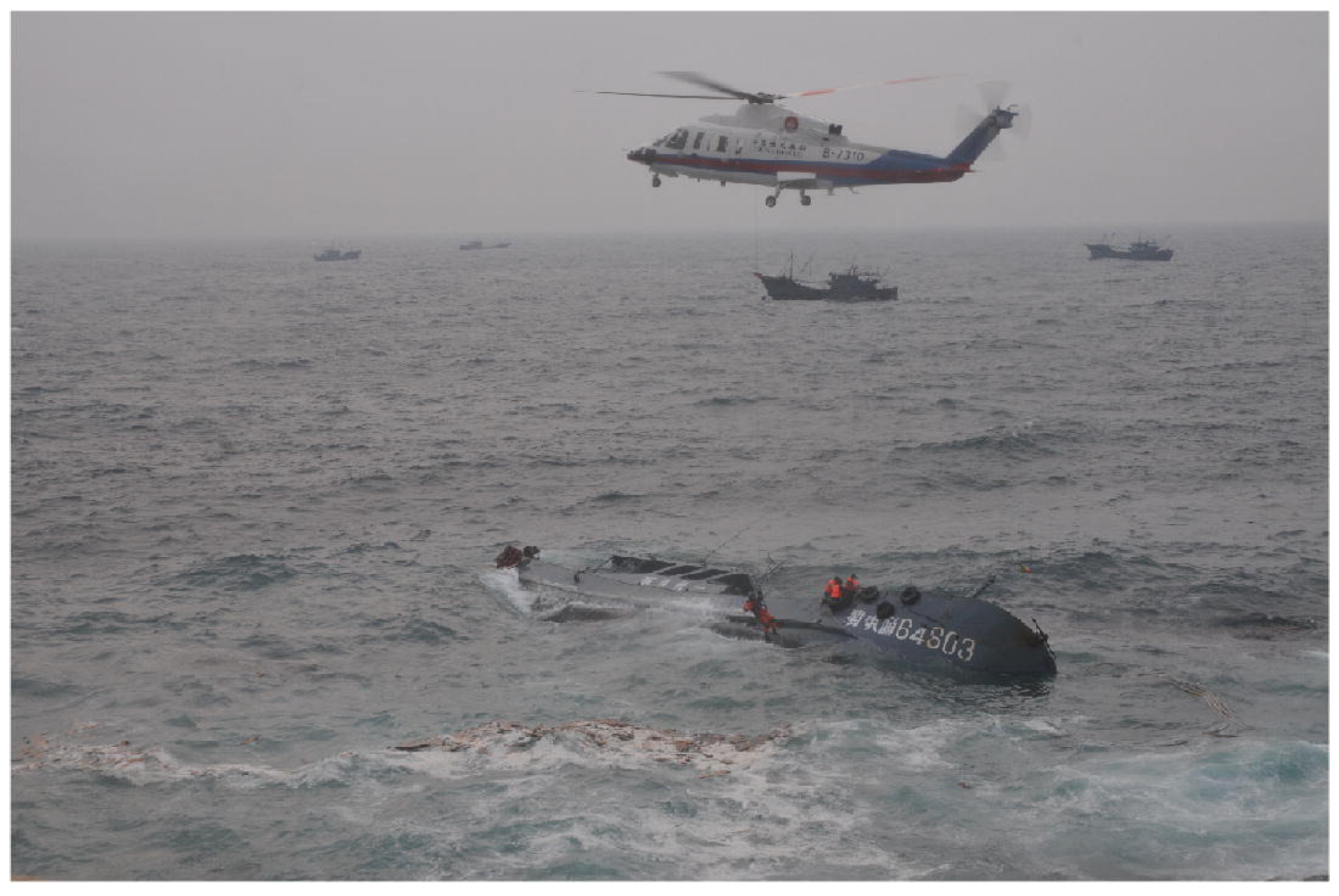
- Serra, M.; Sathe, P.; Rypina, I.; Kirincich, A.; Ross, S.D.; Lermusiaux, P. Search and rescue at sea aided by hidden flow structures. Nat. Commun. 2020, 11, 2525. [Google Scholar] [CrossRef] [PubMed]
- Li, S.; Chen, H.; Wang, M.; Heidari, A.A.; Mirjalili, S. Slime Mould algorithm: A new method for stochastic optimization. Future Gener. Comput. Syst. 2020, 111, 300–323. [Google Scholar] [CrossRef]
- Xue, J.; Shen, B. A novel swarm intelligence optimization approach: Sparrow search algorithm. Syst. Sci. Control. Eng. 2020, 8, 22–34. [Google Scholar] [CrossRef]
- Zervoudakis, K.; Tsafarakis, S. A mayfly optimization algorithm. Comput. Ind. Eng. 2020, 145, 106559. [Google Scholar] [CrossRef]
- Arora, S.; Singh, S. Butterfly optimization algorithm: A novel approach for global optimization. Soft Comput. 2019, 23, 715–734. [Google Scholar] [CrossRef]
- Feng, Y.; Deb, S.; Wang, G.G.; Alavi, A.H. Monarch butterfly optimization: A comprehensive review. Expert Syst. Appl. 2021, 168, 114418. [Google Scholar] [CrossRef]
- Peña-Delgado, A.F.; Peraza-Vázquez, H.; Almazán-Covarrubias, J.H.; Torres Cruz, N.; García-Vite, P.M.; Morales-Cepeda, A.B.; Ramirez-Arredondo, J.M. A Novel Bio-Inspired Algorithm Applied to Selective Harmonic Elimination in a Three-Phase Eleven-Level Inverter. Math. Probl. Eng. 2020, 2020, 8856040. [Google Scholar] [CrossRef]
- Lin, Z.; Yue, M.; Chen, G.; Sun, J. Path planning of mobile robot with PSO-based APF and fuzzy-based DWA subject to moving obstacles. Trans. Inst. Meas. Control. 2022, 44, 121–132. [Google Scholar] [CrossRef]
- Li, X.; Wu, D. An Improved Method of Particle Swarm Optimization for Path Planning of Mobile Robot. J. Control. Sci. Eng. 2020, 2020, 3857894. [Google Scholar] [CrossRef]
- Song, B.; Wang, Z.; Zou, L. An improved PSO algorithm for smooth path planning of mobile robots using continuous high-degree Bezier curve. Appl. Soft Comput. 2021, 100, 106960. [Google Scholar] [CrossRef]
- Liu, H.; Chen, Z.; Tian, Y.; Wang, B.; Yang, H.; Wu, G. Evaluation method for helicopter maritime search and rescue response plan with uncertainty. Chin. J. Aeronaut. 2021, 34, 493–507. [Google Scholar] [CrossRef]
- Jamil, M.; Yang, X.S.; Zepernick, H.J. 8—Test Functions for Global Optimization: A Comprehensive Survey. In Swarm Intelligence and Bio-Inspired Computation; Elsevier: Amsterdam, The Netherlands, 2013; pp. 193–222. [Google Scholar] [CrossRef]
- Locatelli, M. A Note on the Griewank Test Function. J. Glob. Optim. 2003, 25, 169–174. [Google Scholar] [CrossRef]
- Surjanovic, S.; Bingham, D. Virtual Library of Simulation Experiments: Test Functions and Datasets. Available online: http://www.sfu.ca/~ssurjano (accessed on 15 November 2023).
- Acampora, G.; Schiattarella, R.; Vitiello, A. Using quantum amplitude amplification in genetic algorithms. Expert Syst. Appl. 2022, 209, 118203. [Google Scholar] [CrossRef]
- Goldberg, D.E. Genetic Algorithms in Search, Optimization and Machine Learning; Addison-Wesley Professional: Boston, MA, USA, 1989; ISBN 978-0-201-15767-3. [Google Scholar]
- Darwin, C. The Origin of Species, 1st ed.; Prakash Books India Pvt Ltd.: New Delhi, India, 2013; ISBN 13 978-8172344887. [Google Scholar]
- Zhong, R.Y.; Xu, X. Intelligent Manufacturing in the Context of Industry 4.0: A Review. Engineering 2017, 3, 616–630. [Google Scholar] [CrossRef]


| Test Function | Ackley | Sphere | Schaffer | Schwefe |
|---|---|---|---|---|
| Iteration | 5000 | 5000 | 5000 | 5000 |
| MSRA Error | 3.55 × | 2.59 × | 6.49 × | 2.55 × |
| SMA Error | 2.31 × | 2.39 × | 4.19 × | 118.44 |
| GA Error | 8.71 × | 1.45 × | 1.34 | 4.343 |
| Test Function | Ackley | Sphere | Schaffer | Schwefe |
|---|---|---|---|---|
| Iteration | 20,000 | 20,000 | 20,000 | 20,000 |
| MSRA Error | 3.55 × | 4.40 × | 0 | 3.32 × |
| SMA Error | 0 | 0 | 9.73 × | 4.12 × |
| GA Error | 6.30 × | 3.43 × | 9.72 × | 2.90 × |
| Running Sequence | 1st | 2nd | 3rd | |||
|---|---|---|---|---|---|---|
| Iteration | 10,000 | 10,000 | 10,000 | |||
| Error | Location | Error | Location | Error | Location | |
| MSRA | 3.64 × | (−420.9688, −420.9688) | 5.06 × | (−420.9692, −420.9692) | 9.40 × | (−420.9680, −420.9692) |
| SMA | 368 | (−453.7, 500) | 392.6 | (−432.5, −241.1) | 137.7 | (−409.3, 306.9) |
| Running Sequence | 1st | 2nd | 3rd | |||
|---|---|---|---|---|---|---|
| Iteration | 100,000 | 100,000 | 100,000 | |||
| Error | Location | Error | Location | Error | Location | |
| MSRA | 0 | (−1.2129 × , 1.2129 × ) | 0 | (−1.21291 × , 1.21291 × ) | 0 | (−1.1852 × , 1.2129 × ) |
| SMA | 9.717 × | (3.13559095 0.11067923) | 9.716 × | (2.31053014, −2.12505417) | 9.721 × | (−2.20396153, 2.23757538) |
| 1 | Y-axis screw-rod-1 | C1 | Resonant capacitance at the transmitter |
| 2 | X-axis screw-rod | C2 | Resonant capacitance at the receiver |
| 3 | 15V DC regulated power supply | DSP | Digital signal processing |
| 4 | Gate-drive-circuit-1 | L1 | Transmitting coil |
| 5 | Gate-drive-circuit-2 | L2 | Receiving coil |
| 6 | Full-bridge inverter circuit module | MCU | Microcontroller unit |
| 7 | Full-bridge rectifier filter circuit in output module | RL | Load resistance in the output module |
| 8 | Output voltage current sampling circuit | X-SMD | Stepper motor driver in X-axis |
| 9 | Y-axis screw-rod-2 | Y-SM | Stepper motor in Y-axis |
| 10 | Upper computer; | Y-SMD | Stepper motor driver in Y-axis |
| X Coordinate, m | Y Coordinate, m | Input Voltage, Ui, V | Input Current, Ii, A | Output Voltage, Uo, V | Output Current, Io, A | WPT Efficiency , % | Mutual Inductance, M, H |
|---|---|---|---|---|---|---|---|
| −0.312 | −0.139 | 400 | 7.94 | 405.97 | 5.8 | 74.13 | 6.48 × |
| −0.292 | −0.139 | 400 | 7.94 | 408.53 | 5.84 | 75.07 | 6.65 × |
| −0.272 | −0.139 | 400 | 7.94 | 410.51 | 5.86 | 75.8 | 6.78 × |
| −0.252 | −0.139 | 400 | 7.95 | 412.22 | 5.89 | 76.37 | 6.89 × |
| −0.232 | −0.139 | 400 | 7.95 | 413.49 | 5.91 | 76.82 | 6.97 × |
| −0.212 | −0.139 | 400 | 7.93 | 414.05 | 5.91 | 77.18 | 7.04 × |
| −0.192 | −0.139 | 400 | 7.94 | 414.9 | 5.93 | 77.39 | 7.09 × |
| −0.172 | −0.139 | 400 | 7.94 | 415.11 | 5.93 | 77.51 | 7.11 × |
| There are 600 lines of data in total; the middle part has been omitted; the following is the last 10 lines of the data | |||||||
| −0.057 | 0.017 | 400 | 7.94 | 422.53 | 6.04 | 80.30 | 7.74 × |
| −0.057 | 0.018 | 400 | 7.94 | 422.69 | 6.04 | 80.36 | 7.75 × |
| −0.057 | 0.019 | 400 | 7.94 | 422.60 | 6.04 | 80.33 | 7.74 × |
| −0.057 | 0.020 | 400 | 7.94 | 422.54 | 6.04 | 80.31 | 7.74 × |
| −0.057 | 0.021 | 400 | 7.94 | 422.60 | 6.04 | 80.33 | 7.74 × |
| −0.057 | 0.022 | 400 | 7.94 | 422.67 | 6.04 | 80.36 | 7.74 × |
| −0.057 | 0.023 | 400 | 7.94 | 422.53 | 6.04 | 80.33 | 7.74 × |
| −0.057 | 0.002 | 400 | 7.94 | 422.81 | 6.04 | 80.41 | 7.76 × |
Disclaimer/Publisher’s Note: The statements, opinions and data contained in all publications are solely those of the individual author(s) and contributor(s) and not of MDPI and/or the editor(s). MDPI and/or the editor(s) disclaim responsibility for any injury to people or property resulting from any ideas, methods, instructions or products referred to in the content. |
© 2023 by the authors. Licensee MDPI, Basel, Switzerland. This article is an open access article distributed under the terms and conditions of the Creative Commons Attribution (CC BY) license (https://creativecommons.org/licenses/by/4.0/).
Share and Cite
Zheng, J.; Jettanasen, C.; Chiradeja, P. Performance and Application Analysis of a New Optimization Algorithm. Computation 2024, 12, 1. https://doi.org/10.3390/computation12010001
Zheng J, Jettanasen C, Chiradeja P. Performance and Application Analysis of a New Optimization Algorithm. Computation. 2024; 12(1):1. https://doi.org/10.3390/computation12010001
Chicago/Turabian StyleZheng, Junlong, Chaiyan Jettanasen, and Pathomthat Chiradeja. 2024. "Performance and Application Analysis of a New Optimization Algorithm" Computation 12, no. 1: 1. https://doi.org/10.3390/computation12010001
APA StyleZheng, J., Jettanasen, C., & Chiradeja, P. (2024). Performance and Application Analysis of a New Optimization Algorithm. Computation, 12(1), 1. https://doi.org/10.3390/computation12010001