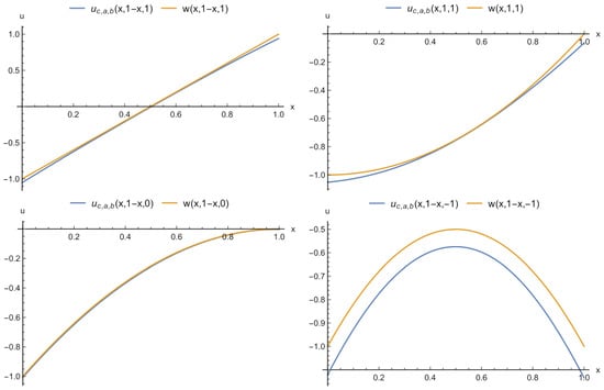
Abstract
This article examines the possibilities of adapting approximate solutions of boundary value problems for differential equations using physics-informed neural networks (PINNs) to changes in data about the physical entity being modelled. Two types of models are considered: PINN and parametric PINN (PPINN). The former is constructed for a fixed parameter of the problem, while the latter includes the parameter for the number of input variables. The models are tested on three problems. The first problem involves modelling the bending of a cantilever rod under varying loads. The second task is a non-stationary problem of a thermal explosion in the plane-parallel case. The initial model is constructed based on an ordinary differential equation, while the modelling object satisfies a partial differential equation. The third task is to solve a partial differential equation of mixed type depending on time. In all cases, the initial models are adapted to the corresponding pseudo-measurements generated based on changing equations. A series of experiments are carried out for each problem with different functions of a parameter that reflects the character of changes in the object. A comparative analysis of the quality of the PINN and PPINN models and their resistance to data changes has been conducted for the first time in this study.
1. Introduction
The classical approach to mathematical modelling of real objects can be divided into two stages. In the first stage, a mathematical model is formulated based on the study of physical processes. Typically, this model consists of differential equations and additional conditions such as initial or boundary conditions. The second stage involves the construction of numerical solutions for these equations, as well as the visualisation of solution graphs.
In cases where the differential equations and boundary conditions precisely capture the behaviour of the simulated object, various classical methods have been developed and extensively validated. For instance, a range of classical Runge–Kutta methods for ordinary differential equations, combined with techniques like the shooting method for boundary value problems [1], have been formulated. Similarly, grid-based and finite element methods [2,3] have been devised for solving partial differential equations.
In recent years, there has been a growing emergence of a new paradigm in mathematical modelling that incorporates not only differential equations but also data to construct mathematical models. However, it is worth noting that certain tasks traditionally considered incorrect [4] in this context have become subjects of discussion. The exploration of this paradigm and the examination of specific tasks associated with it can be found in various scholarly works, including [5,6,7,8,9,10,11]. This direction has gained additional relevance in the current age of Industry 4.0 [12] accompanied by the widespread introduction of Cyber–Physical Systems and Digital Twins [13]. The development of sensor technologies makes it possible to obtain data about the object of modelling in real time and to adapt the model to changes in a timely manner. The hybrid approach can provide a more robust and accurate model that mitigates some of the disadvantages of using purely physics-based or data-driven models [14,15].
In certain situations where knowledge of the differential equation and boundary conditions is imprecise or incomplete, and measurement results are available, neural networks have proven to be more effective. However, it is important to note that using neural networks often requires a lengthy and resource-intensive training process. Another class of problems in which neural networks are recommended is when the equation’s parameters undergo unknown variations and only the measurement results are accessible during dynamic processes. The present paper investigates a similar problem, thereby contributing to the understanding of such problems.
Solving differential equations by means of neural networks originates at the end of the 20th century [16,17]. Our first studies [5,18] on this topic were published in 2005, when different terminology was used. In 2019, the publication [19] of Raissi, Perdikaris, and Karniadakis brought wide fame and a recognisable name PINN (Physics-Informed Neural Networks) to neural network models described using differential equations and obtained by minimising a specific loss function. Since then, a large number of articles have been published annually on solving problems involving differential equations using machine learning methods.
In many cases, the problem formulation involves parameters that exhibit variations within a certain range. For instance, properties like density, coefficients of thermal conductivity, elasticity, and others may not be precisely known for real media. Additionally, factors such as object size and ambient temperature may also exhibit variability. In such scenarios, the task of constructing parametric models arises, either to investigate the solution’s behaviour dependent on a specific parameter or to estimate the parameter value using measurement data.
The classical approach traditionally involves obtaining a numerical solution for the problem using a representative set of parameters. However, our proposed approach [20,21,22] presents an alternative method. It allows us to search for a solution in the form of a neural network function, where the relevant parameters are included as arguments.
There are not only PINNs to which several recent reviews [23,24] are devoted but also more general issues [8,9,10] covering a new modelling paradigm and hybrid models combining physics and heterogeneous data.
In the paper [6], we presented our approach to constructing a neural network model based on all available information (differential equations, boundary conditions, measurement data, etc.) about a stationary object. In this paper, we focused on another problem that arises when modelling real objects. It takes into account the possibility of their change during operation. These changes can be considered smooth increases or decreases, as well as sharp jumps in the values of parameters corresponding to any physical properties of the simulated object, and its functioning or operation conditions. Mostly, there are tasks when parameters characterise the domain shape or boundary condition for differential equations [25].
The benchmark problems we solve in this paper have been chosen in such a way as to study various aspects of changes in the modelling object. Pseudo-measurements used to adapt the constructed models are generated based on known analytical solutions. Relevant are the problem statements when the object is described using equations which are not quite accurate. Thus, in the second benchmark problem, the initial model is constructed based on an ordinary differential equation, while in fact, the modelling object satisfies a partial differential equation according to which the corresponding measurements are generated. The paper in [26] focuses on the learning of a dynamical system for making forecasts, particularly when certain variables are unobserved by utilising physics-based and data-driven modelling. In [27], surface uncertainties are regarded as one of the limiting factors of physics-based contact modelling methods. The problem statement is close to multi-fidelity data-driven modelling with approximate governing equations. One of the solutions is estimating the current model error and further incorporating it in the equation as a corrective term [28]. Another option, besides data-driven discovery of the equations, in the case of modelling unknown or partially known dynamics, is dynamical system identification [29]. But, they do not discuss data-driven real-time adaptation of a used model and the qualitative behaviour of the solution does not change when the parameter changes over time. At the same time, it is interesting to check the adaptive properties of PINNs on a problem when the solution qualitatively changes its nature. To this end, we consider a partial differential problem in which a parameter change leads to a shift in the type of equation from elliptic to hyperbolic. There is some work devoted to a certain type, for example, elliptic [30]. The study of mixed-type problems using PINNs is found on the example of stochastic partial differential equations [31].
In this paper, we focused on comparing two types of neural networks: PINNs and parametric PINNs (PPINs). Adaptive properties of these networks are analysed and compared on each of the benchmark problems. PINNs are constructed with fixed parameter values using the methods described in our earlier work [5,18], and the PPINNs include the parameters for the number of input variables [6,20,21,22,32]. Including system parameters as an input to the model allows for providing real-time simulation for a range of problem settings and decreases computation time [33]. Moreover, solving parametrised governing systems can be used in a wide variety of complex systems [34].
2. Materials and Methods
Let us consider a boundary-value differential problem in a general formulation for both ordinary and partial differential equations:
where ; , ; is a differential operator; and is a valid operator that sets boundary conditions.
The general neural network approach to solving this problem, which has recently received the conventional name physics-informed neural network (PINN) approach, consists in adjusting the parameters (weights) of a neural network during the process of minimising the loss function corresponding to the task under question.
Implying changes in the object described using system (1), we introduce into the formulation of the problem a certain parameter , which takes acceptable values in the corresponding area with appropriate d:
Some values of the parameter where time , can change the nature of the problem, for example, reduce its dimension or determine the type of differential operator. Here, , .
In this paper, we consider the situation when, initially, the object is described using system (2) at a fixed value of the parameter . Then, changes begin to occur, with the object corresponding to a variation in the parameter value. Meanwhile, the information about these changes comes to us only in the form of real-time measurements. The question arises how well a neural network model can adapt to such changes. To answer this question, we consider the PINN (3) and PPINN (5) models, which are illustrated in Figure 1.
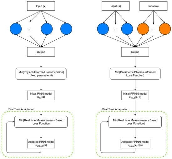
Figure 1.
Schematic of the PINN (left) and PPINN (right) for solving differential equations and adapting to measurements.
In the first case, the initial PINN model is constructed for system (1) and represents the output of a neural network with one hidden layer of the form
The weights of the network (parameters , q depends on a certain basis function ) are adjusted by minimising the physics-informed loss function
for a known fixed initial value of the parameter . Here, is a training sample randomly selected using a uniform distribution inside the domain with the condition of regeneration (resampling) according to the selected neural network learning algorithm. The boundary condition training sample is some grid on . A is a positive penalty parameter.
The initial PPINN model has the form
The weights of the network (parameters , , ; depend on a certain basis function ) are selected by minimising the physics-informed loss function corresponding to system (2). Here, an additional parameter vector is introduced to emphasise the difference between basis functions for PINN and PPINN. Specifically,
where and are the training samples uniformly distributed on and some grid on , respectively. A is a positive penalty parameter.
The adaptation of the obtained PINN and PPINN models consists in adjusting the weights of the solution (3) and the parameter of the solution (5) during the minimisation of real-time measurement-based loss functions:
and
respectively. Here, are the measurement data at the time point .
PINN is trained with a fixed initial parameter value. PPINN incorporates the parameter as an additional input variable and is trained using a particular set of initial parameter variations. Subsequently, the parameter continues to change, but these changes are not utilised for training the networks. Instead, “measurement” data are generated according to a predefined law governing the parameter variation. PINNs are further trained to optimise its performance by minimising a given objective function. In contrast, PPINN focuses on parameter identification, which consequently influences the output function as well.
Selecting appropriate penalty factor A in (4,6) presents a challenge in this context, and various approaches have been proposed to address this issue. In [35], adaptive weights are suggested, where the penalty parameter is updated during network training steps using a predetermined formula. In [36], updating the weights after a certain number of training epochs is proposed to achieve a balanced contribution from each term. In [37], the influence of the parameter on the learning rate is evaluated and a fixed value is employed for obtaining the final solution.
3. Benchmark Problems
3.1. Modelling Bending of the Cantilever Rod under Load
In our initial task, we focused on studying the deflection of a cantilever rod when subjected to a load. To develop an approximate differential model, we made several assumptions about the rod’s properties. Specifically, we treated the rod as an infinitely thin, homogeneous, linearly elastic structure that was initially straight.
By considering the equation describing the large static deflection of such a rod under the influence of distributed and concentrated forces projected onto the tangent of the deflection curve, we solve a differential equation:
where , ; D is a constant bending stiffness; denotes the angle of inclination of the tangent to the curve describing the rod; z represents the natural coordinate of the curved axis of the rod measured from the sealing; m denotes the weight of the rod; and F represents force acting on the unfixed rod end. See Figure 2.
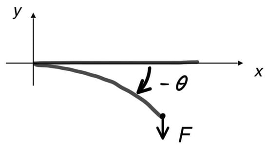
Figure 2.
Bending of the Cantilever Rod under Load Scheme.
Then, the boundary conditions has the form of
The relationship between the angle and the coordinates of the points on the rod is described using the equalities
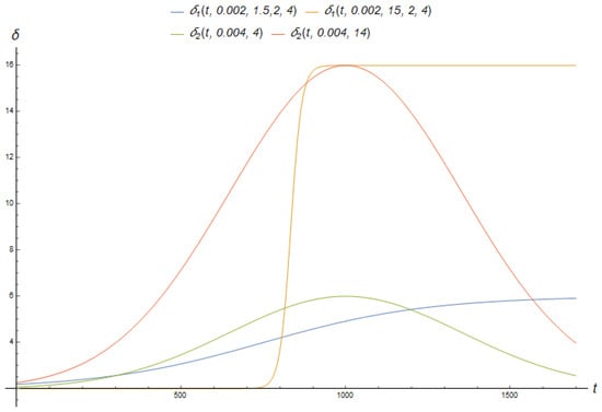
In order to generate pseudo-measurement data, various forms of parameter dependencies on time, represented by different functions , are employed. Each function exhibits unique characteristics, which are depicted in Figure 3 and described below.
- The first variations in the parameter’s time dependence correspond to a transient process characterised by a maximum speed within a specific time interval, eventually reaching a state of saturation.
- The subsequent time dependence of the parameter simulates a short-term deviation from its stationary value. We tested the dependencies of the parameter measurement in this context.
3.2. Non-Stationary Problem of a Thermal Explosion in the Plane-Parallel Case
The second task we considered is the non-stationary problem of a thermal explosion in the plane-parallel case [38] under the assumption that the reaction has one stage and is irreversible; it is not accompanied by phase transitions, and it proceeds in a stationary medium.
It is quite accurately described with a partial differential equation [39]:
where is an analytical solution to the system (15) in the case of .
It is assumed that the non-stationary nature of the object under consideration is unknown and it satisfies a time-independent boundary value problem for an ordinary second-order differential equation [38]:
This problem is interesting because we know the exact solution, the area of existence of the solution (), and the parameter values for which the solution of the problem does not exist (). Here, the change interval of the variable is derived from the problem statement and is linked to the shift towards a dimensionless coordinate. In the case of small parameter values, it is quite convenient to obtain a solution by using asymptotic methods. Furthermore, in order to attain a low relative error for these parameter values, modifying the loss function becomes necessary. These alterations are specific to the task at hand, making it challenging to utilise this problem as a demonstration of the general methodology. In the case of small parameter values, it is quite convenient to obtain a solution by using asymptotic methods. Obviously, the operating mode of a real reactor should not approach the limits of stability. The low reaction rate corresponding to small parameter values also does not meet real operating modes due to low efficiency. Therefore, for training the parametric model, we assume that and investigate the possibility of adapting PINN models when changing the parameter .
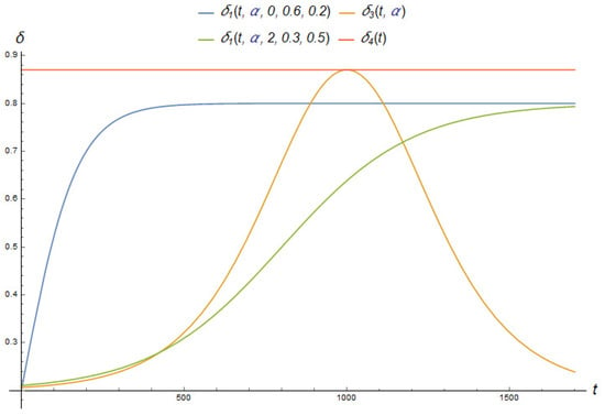
To generate pseudo-measurement data, different variants of the parameter dependence on time are used. Every function has its own features, which Figure 4 illustrates.
- The first variant of the time dependence of the parameter is a special case of (12) and corresponds to the transition process, which has a maximal speed at the initial moment and becomes saturated:
- The second function change simulates a short-term deviation of the parameter from a stationary value:
- The third dependence is also a special case of (12) and differs from the first two via a time shift in the dramatical parameter change:
- The last dependence is a jump at the initial moment of time into a domain close to the boundary of the solution stability. Note that the parameter value in this case goes beyond the interval at which parametric PINN models have been trained. It is set by
3.3. The Problem with an Equation of Mixed Type
Let us consider the problem of a partial differential equation where changing a parameter leads to a shift in the type of equation from elliptic to hyperbolic. The nature of a solution changes accordingly. More specifically, it is the boundary value problem in the unit square ():
The exact solution of (20) is
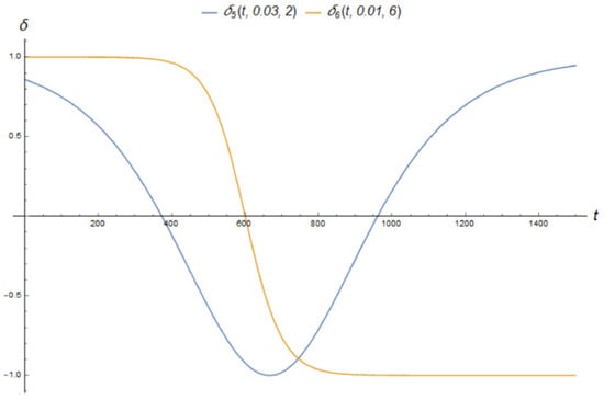
It is assumed that the parameter can change within the interval . We also consider various dependencies of parameter on time (see Figure 5):
- The first one causes the short-term deviation of the parameter from a stationary value:
- The next dependence is sigmoid with a time shift (delay). Thus, we consider a situation when, during the operation of algorithm, there is a transition from one stationary state to another. The parameter changes according to
4. Computational Experiments and Results
For all tasks, the minimisation of loss functions (4) and (6) is carried out according to the nonlinear optimisation algorithm RProp [40] with the regeneration (resampling) [41] of test (training) points every five steps of the optimisation process. RProp implements a localised adaptation of weight updates based on the error function’s behaviour. Unlike other adaptive techniques, the impact of the RProp adaptation process is not affected by the unpredictable influence of derivative magnitude but solely relies on the temporal pattern of its sign. The resampling allows us to avoid neural network overfitting that distinguishes our approach from the classical case of learning in collocation points. Regeneration means selecting new training points by generating a sample from the uniform distribution on domains and , respectively. For the second term of the loss function, uniform grids on and are used.
As it is mentioned above, we generate pseudo-measurements for all tasks by calculating solution values at points of time , indicating the time in seconds since the start of the adaptation algorithm. To address the first task, surrogate measurement data have been utilised by selecting values of the solution to the problem:
Thus, for the second problem is the values of the solution to (14) in the case of a fixed parameter . All solutions are based on an inaccurate description of the object using Equation (15), and after adaptation, the resulting solution is compared with the solution of the problem (14).
For the third task, we have used the exact solution (21) to the system (20) for . We take for the second and third tasks and for a special experiment with the mixed-type problem.
The adjustment of neural network parameters occurs during the minimisation of discrepancies (7) and (8) for the PINN and PPINN models, respectively. For each model, five steps of the minimisation algorithm are executed.
4.1. Modelling Bending of the Cantilever Rod under Load
4.1.1. PINN Model
To address the given problem, we utilise the PINN (3), specifically a solution to (9)–(10)
when is fixed. In this case, we employ a Gaussian basis function
and also investigate a perceptron neural network with a basis function:
The parameters and of the PINN are optimised by minimising the loss
Here, the test points are randomly selected using a uniform distribution within the interval [0, 1]. The penalty parameter A is computed during network initialisation to maintain consistent ordering of the terms in the loss function.
4.1.2. PPINN Model
As an approximate PPINN (5) solution, we constructed a neural network:
In our investigation, we explored various basic functions, and the most favourable outcomes were achieved when selecting basic functions in the form described by following equation:
and for comparison with Gaussian PINN, we have
The weights of the network are carefully chosen by minimising the error function:
Here, are test points randomly selected using a two-dimensional uniform distribution inside the rectangle . In computational experiments, a value has been selected for both the PINN and PPINN models. A is a positive penalty parameter.
4.1.3. Initial PINN and PPINN Models
Initially, PINN and PPINN have been trained without considering dynamically changing data. For the PINN (3) approximation, we successfully achieved a sufficiently small error by utilising a network with two neurons. By selecting a specific parameter value , the resulting networks are
for Gaussians and
for the basis function (27).
The accuracies of the solutions are further illustrated in Figure 6. Subsequently, these networks are utilised as initial approximations to handle dynamic changes in the data.

Figure 6 clearly demonstrates that the perceptron PINN achieves notably higher accuracy. However, subsequent computational experiments reveal that this higher accuracy does not necessarily translate to improved performance in processing dynamic data.
At the specified parameter value , we achieved a neural network approximation for Gaussians:
The absolute error of this approximation remains below 0.006, demonstrating the potential accuracy that can be achieved as the parameter increases to .
On the other hand, the PPINNs necessitate a larger number of neurons (terms) to achieve an acceptable approximation, and it yields significantly lower accuracy. Further, we present the results for and . We have omitted the detailed formulas for these models. When utilising a reduced number of neurons, the outcomes are notably unsatisfactory.
Figure 7 displays similar plots for PPINNs with 30 neurons, illustrating significantly improved model accuracy. As a result, the use of networks with 10 neurons was discontinued in subsequent experiments. For PPINNs, the accuracy of the perceptron model is about the same as that with radial basis functions.
4.1.4. Adapting PINN and PPINN Models
Further, we have performed computational experiments to adapt the neural networks constructed in the first step, PINN and PPINN, using dynamically changing data. To generate the data, we utilised model (24) with different parameter dependency options based on the iteration number i.
The time needed to produce five steps for the minimisation of a loss function (6) was denoted by . Then, at each number of adaptation process for each dependence , the mean squared error (MSE) was calculated for each model at 100 points evenly distributed over the segment
where is the solution to the system (9) and (10) for (12) and (13).
At each consecutive point i during the adaptation process to pseudo-measurements, Figure 8 showcases the relationship between the dependency on time and the corresponding MSE of the adapting models.
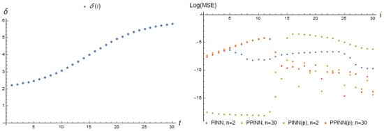
Figure 8.
Parameter dependence (12) and log(MSE) (36) of corresponding real-time adapting PINN, basis functions (26), and PINNp, basis functions (27), with 2 neurons and PPINN, basis functions (30), and PPINNp, basis functions (31), with 30 neurons of a hidden layer at each adaptation step i for tasks (9) and (10).
Figure 8 demonstrates that the perceptron PINN exhibits substantial advantages during the initial step, but these advantages diminish when there is a significant change in the parameter .
Figure 9, Figure 10 and Figure 11 present comparable results for dependencies and , respectively, and confirm that the perceptron does not demonstrate noteworthy advantages.
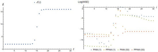
Figure 9.
Parameter dependence (12) and log(MSE) (36) of corresponding real-time adapting PINN(1), basis functions (26), with 2 neurons; PPINN(1), basis functions (30), with 30 neurons of a hidden layer at each adaptation step i; PINN(50), basis functions (26), with 2 neurons; and PPINN(50), basis functions (30), with 30 neurons. The data generated using the model (24), with the parameter change law during 50 iterations of training, occurring between the moments of data acquisition for task (9) and (10).
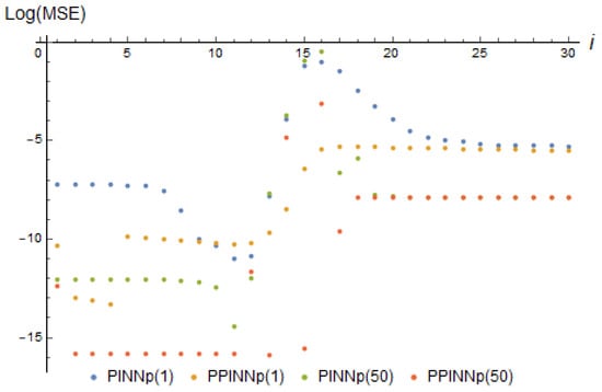
Figure 10.
log(MSE) (36) of corresponding real-time adapting PINNp(1), basis functions (27), with 2 neurons; PPINNp(1), basis functions (31), with 30 neurons of a hidden layer at each adaptation step i; PINNp(50), basis functions (27), with 2 neurons; and PPINNp(50), basis functions (31), with 30 neurons. The data generated using the model (24) with the parameter change law during 50 iterations of training, occurring between the moments of data acquisition for task (9) and (10) parameter dependence (12).
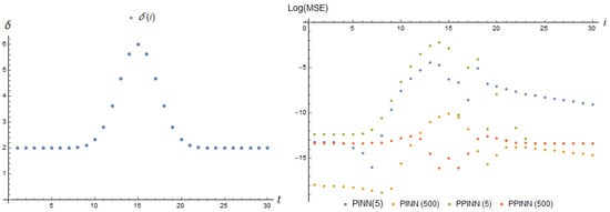
Figure 11.
Parameter dependence (13) and log(MSE) (36) of corresponding real-time adapting PINN, basis functions (26), with 2 neurons and PPINN, basis functions (30), with 30 neurons of a hidden layer at each adaptation step i for tasks (9) and (10); 5 and 500 iterations of training are considered between the moments of data reception.
The presented results lead us to the conclusion that the error in the PINN model is primarily attributed to its adaptive characteristics. Conversely, for PPINN models, the main source of errors can be traced back to inaccuracies in the initial training process. These findings shed light on the distinct sources of errors in the PINN (3) and PPINN (5) models, emphasising the importance of considering the specific characteristics and training procedures when analysing and improving their performance.
The time-dependent behaviour of and simulates a short-term deviation of the parameter from its stationary value. In Figure 11, Figure 12 and Figure 13, we observe how the dependencies and change over time and its impact on the mean squared error (MSE) of the adapting models with different basis functions.
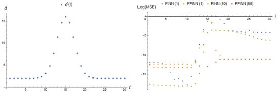
Figure 12.
Parameter dependence (13) and log(MSE) (36) of according real-time adapting PINN, basis functions (26), with 2 neurons and PPINN, basis functions (30), with 30 neurons of a hidden layer at each adaptation step i for tasks (9) and (10); 5 and 50 iterations of training are considered between the moments of data reception.

Figure 13.
log(MSE) (36) of corresponding real-time adapting PINNp, basis functions (27), with 2 neurons and PPINNp, basis functions (31), with 30 neurons of a hidden layer at each adaptation step i for tasks (9) and (10); 5 and 500 iterations of training are considered between the moments of data reception, for parameter dependencies (13) (left), (right).
Figure 13 clearly demonstrates that the perceptron does not possess any advantages over a network employing a Gaussian basis function. As a result, the perceptron is not employed in the subsequent experiments.
Upon analysing the graphs presented in Figure 11 and Figure 12, we observe a sharp increase in the error of both the PINN and PPINN models at the moment of the highest rate of parameter increase. This finding reaffirms that the adaptive characteristics of these models remain the primary cause of their error. Notably, the error of the PINN model does not significantly decrease even with an increase in the number of training iterations between data points, particularly when the parameter experiences a substantial increase. This suggests that the main source of errors for PINN (3) models is the instability of the learning process when confronted with drastic changes in the data. It is worth mentioning that, with a significant increase in the parameter, some model runs were unsuccessful, indicating that PINN can exhibit high error rates despite prolonged training. On the other hand, the error of the PPINN model exhibits a substantial decrease with an increase in the number of training iterations between data points, especially in the case of a significant parameter increase. Consequently, for PPINN (5) models, errors primarily stem from inaccuracies in the initial training phase of the network.
4.2. Non-Stationary Problem of a Thermal Explosion in the Plane-Parallel Case
4.2.1. PINN Model
The PINN parameters , were adjusted by minimising the loss function:
The penalty parameter A was computed during network initialisation to maintain consistent ordering of the terms in the loss function.
4.2.2. PPINN Model
As an approximate PPINN to the (5) solution, we constructed a PPINN solution to (15) that depends on the parameter . Thus, we chose the basis function of the form
The corresponding loss function has the form
In computational experiments for both the PINN and PPINN models, the number of test points has been selected to train initial networks. The PPINNs have been trained on the parameter change interval . The positive penalty parameter A was computed during network initialisation to maintain consistent ordering of the terms in the loss function.
4.2.3. Initial PINN and PPINN Models
A non-parametric PINN solution to the task (15) at a fixed parameter value is sufficiently accurate even in the case of two neurons of a hidden layer. Thus, Figure 14 illustrates an absolute error and compares the PINN approximation
with the exact solution to a system (15) at .

In the case of , the PINN (3) solution
has an absolute error that does not exceed 0.0013. Thus, it is a desired result for the PINN with two neurons in the case of the growth of the parameter from to during the adaptation process.
The parametric PINN (5) requires a larger number of neurons (terms) n for an acceptable approximation and gives a lower accuracy. The one with neurons of a hidden layer has the form
We have not given the formula for the output of the 30-neuron PPINN because of its bulkiness.
4.2.4. Adapting PINN and PPINN Models
We have conducted numerical experiments for various initial PINN models and time dependences of the parameter . We studied the initial PINN model (41) with 2 neurons and PPINN models with 10 (43) and 30 neurons of a hidden layer discussed above.
Similar to the previous approach, for each adaptation process number , we evaluated the mean squared error (MSE) of the approximate solution at 100 points evenly distributed over the segment . This evaluation was performed for each dependency
where is the solution to the system (14) for .
Figure 16 illustrates the dependency on time and the corresponding MSE of the adapted models under consideration at consecutive points i of adaptation to pseudo-measurements. The MSE of the adapted PINN model increased sharply at the initial moment, reached a maximum, and quickly decreased to small values with stabilisation of the parameter near a new value. The error of both PPINN models had a similar behaviour. The MSE grew, while tended toward a new stable value. Further, it remained consistently higher than the initial value. Despite a smaller difference in the loss function value of the initial models, the maximal MSE of the PPINN with 10 neurons was about two times greater than that of the PPINN with 30 neurons.
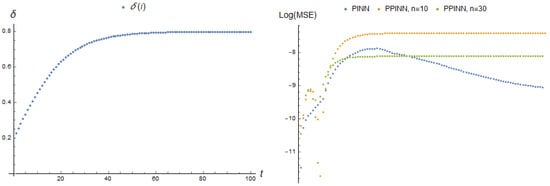
Figure 16.
Parameter dependence and Log[MSE] (44) of corresponding real-time adapting PINN with 2 neurons and PPINN with 10 and 30 neurons of a hidden layer at each adaptation step i.
When the change rate of the parameter increases to , the process of adapting the initial PINN model—the minimisation of loss function (7)—loses stability. The behaviour of the adapting PPINN MSE is similar to that shown in Figure 14 but with much more earlier stabilisation of the error. Its maximal values are presented in Table 1.

Table 1.
max{MSE} for PINN and PPINN adaptive solutions to second problem and various parameter dependencies.
The next dependency (17) that we considered simulates a short-term deviation of the parameter from a stationary value. Figure 17 shows the results for on the parameter change time interval . The maximal MSEs are presented in Table 1.

Figure 17.
Parameter dependence and Log[MSE] (44) of corresponding real-time adapting PINN with 2 neurons and PPINN with 10 and 30 neurons of a hidden layer at each adaptation step i.
We can see that the MSE of the adapting PINN model increases dramatically at the moment of the highest rate of parameter change. Another maximal error is achieved when the parameter value is close to critical . The MSE of the adapting PPINN model loses its stability when the parameter begin to tends to . The maximal error for the PPINN with 10 neurons of a hidden layer is more than an order of magnitude greater than the error for the PPINN with 30 neurons.
We also have studied dependencies like (18). Thus, we consider a situation when the moment of essential parameter change occurs after some time from the start of the adaptive algorithm (see Figure 4) and the different rates of this change. The behaviour of the adapting PPINN MSE is similar to that shown in Figure 15 but with a shift of the maximal error to the right end of the time interval studied. The maximal errors are also presented in Table 1. Even a small increase in the rate of parameter change from 0.025 to 0.03 affects the accuracy of the adapting PINN model.
The last dependence (19) is a jump at the initial time point to the vicinity of the parameter critical value . Note that the parameter value in this case goes beyond the interval at which PPINNs have been trained. Figure 18 represents the MSE of the adapting PINN and PPINN models. The maximum of errors can be found in Table 1. The MSE of the PINN model is maximal at the initial moment when the parameter changes abruptly and decreases sharply when the parameter value is stable. The error of the PPINN models changes slightly, corresponding to the values of the parameter in the neighborhood of . The MSE for the network with a smaller number of neurons is more than an order of magnitude greater than the error for the PPINN with 30 neurons of a hidden layer.

Figure 18.
Parameter dependence and Log[MSE] (44) of according real-time adapting PINN with 2 neurons and PPINN with 10 and 30 neurons of a hidden layer at each adaptation step i.
4.3. The Problem with an Equation of Mixed Type
4.3.1. PINN Model
For a PINN (3) solution to (20) for fixed , we use a Gaussian basis function of two spatial variables:
The PINN parameters and are adjusted by minimising the loss function:
The penalty parameter A is computed during network initialisation to maintain consistent ordering of the terms in the loss function.
4.3.2. PPINN Model
As an approximate PPINN solution, we construct a PINN solution that depends on the parameter . Thus, we chose the basis function of the form
We typically employ the following activation functions. For tasks in this work, various functions have been examined, including those with two tangents and those with two Gaussians. It has been found that the option presented in the article yielded better results. Similar observations were made when tackling other problems, where Gaussian functions were found to be more suitable for spatial variables (in the absence of abrupt solution changes), while hyperbolic tangent functions were more effective for parametrisation.
The corresponding loss function has the form
The penalty parameter A is computed during network initialisation to maintain consistent ordering of the terms in the loss function.
4.3.3. Initial PINN and PPINN Models
The computational experiment for problem (20), as for the previous one, has been carried out in two steps. In the first step, PINN and PPINN have been trained without taking into account dynamically changing data to obtain initial models. Let us start from . The PINN
with four neurons of a hidden layer has a quite small error on the entire domain . The absolute difference between an exact solution and PINN (49) does not exceed 0.02. Figure 19 illustrates their behaviour on the diagonal and the boundary of .
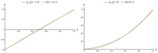
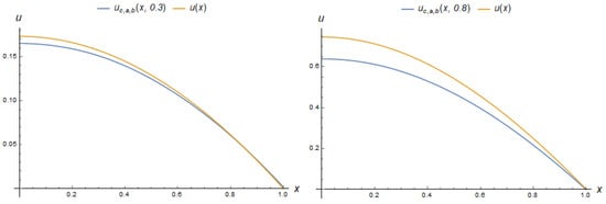
The PPINN (5) requires a much larger number of neurons. We present results for a PPINN with a number of neurons . The network has been trained on the parameter change interval . We do not provide the formula for this model due to its bulkiness. The absolute difference between an exact solution and the PPINN model obtained does not exceed 0.02. The mean square error for 10,000 random points in the domain , was 0.0331. Figure 20 compares the PPINN model with the exact solutions for different values of .
4.3.4. Adapting PINN and PPINN Models
Here, we investigate the adaptation properties of the PINN and PPINNs discussed above in the case of various time dependences of the parameter , as for the previous task. As before, at each number of adaptation process for each dependency , we calculate the MSE for each approximate solution at 10,000 points evenly distributed over
where is a solution to the system (20).
The first variants of the time dependence of the parameter simulate the short-term deviation of the parameter from the stationary value with different rates. For the dependence , the results are presented in Figure 21.
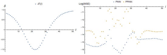
Table 2 contains data about the maximal MSE. It is more than an order of magnitude greater for the PPINN approximate solution than the error of the adaptive PINN model. The first one is large during all times when the parameter value is negative.

Table 2.
max{MSE} for PINN and PPINN adaptive solutions to second problem and various parameter dependencies.
Let us change the rate and time amplitude of parameter deviation. In the case of and for the same dependency , we observe that both adaptive PINN and PPINN errors are maximal simultaneously with the maximal deviation in the parameter from the stationary value and decreases sharply when the parameter value tends to be stable. This is illustrated in Figure 22. Note that the maximum of PINN MSE exceeds more than twice that of the adaptive PPINN solution. The specific values can be found in Table 2.
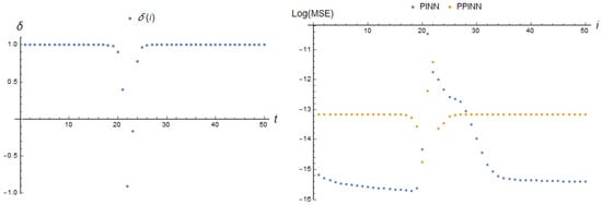
The next two dependencies are sigmoid with a time shift. Thus, we consider a situation when, during the operation of the algorithm, there is a transition from one stationary state to another. The results are presented in Table 2 and illustrated in Figure 23 and Figure 24.

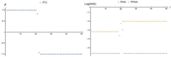
In the case of parameter dependency (23), the PPINN MSE reaches its maximum at the same time as the rate of parameter change. Moreover, it increases during the entire calculation process. The deviation in the PINN MSE decreases during the entire calculation process except for a small section where it can be neglected. The PPINN MSE is more than an order of magnitude greater than that of the adaptive PINN model.
A higher rate of parameter change (compare Figure 23 and Figure 24) leads to other results. For (23), we concur that the PINN MSE has one outlier at the moment of the maximal speed of parameter change and remains stable and small for the rest of the time. The behaviour of the PPINN MSE is also stable almost everywhere besides the small shift at the moment of the maximal rate of parameter change. Note that the maximum of PINN MSE is about three times the error of the PPINN solution.
4.3.5. Experiment with a Small Number of Measurements
It is obvious that a large number of measurements with a stable behaviour of the parameter makes it easy to minimise the loss function of the form (40) for the PINN adaptive model, while the PPINN can be overtrained since, in the optimisation process, just a single parameter of an approximate solution is adjusted for a plenty of data. Thus, it is natural to consider the case when we obtain a small number of measurements at each moment of time. Let the number of measurements be . Moreover, we have chosen specific points .
As a function of parameter change, let us consider that, after a quite smooth shift from one equation type to another, is stable for awhile and . If we compare the predicted values for a solution in four chosen points, we obtain that the maximal absolute error of the PINN solution is s and, for the PPINN, the maximum of error is 0.009. These results may give the impression that the PINN (3) works much more accurately than the PPINN (5), although this is not the case. The MSE after stabilising a parameter value for adaptive PINN and PPINN models are given in the last column of Table 2 and the corresponding solutions are shown in Figure 25.

Thus, the error of the PINN adaptive model with a small number of points where the values of desired function are taken in the adaptation process is poorly characterised by the loss function (7). For an objective assessment of the adaptation error, we need to track the error values in additional test points. The error of the PPINN adaptive solution in the same case is quite well characterised by the loss (8).
5. Conclusions
We have studied the adaptive properties of PINN and PPINN solutions using dynamic real-time data. The ability of the adaptive parametric and classical PINNs to adapt was compared for the first time in this study. This comparison was conducted using problem examples that involved various dependency functions of an unknown dynamic parameter. A series of experiments have been carried out for three benchmark problems with different functions of a parameter that reflects the characteristic of changes in an object. The first problem involved modelling the bending of a cantilever rod under varying loads. In the second task, the initial model was constructed based on an ordinary differential equation, while in fact, the modelling object satisfies a partial differential equation, according to which the corresponding pseudo-measurements have been generated. The third task was to solve a partial differential equation of mixed type depending on time.
Based on computational experiments, we can draw the following conclusions. Both PINN and PPINN approximations have adaptability. The PINN error is caused primarily by its adaptive characteristics. The greatest errors are due to the high rate of parameter change or a sharp jump in its value. The similar behaviour of PPINN MSE suggests that the main source of errors comes from initial training. The larger size of PPINN allows it better to reflect the subtle features of the problem solution over the entire parameter change interval compared with the network with fewer neurons.
At the same time, with a fixed parameter, when solving a differential problem, a simple PINN shows the best result and requires a small number of hidden layer neurons. PPINN requires a large number of neurons, which increases the pre-training time. On the other hand, only one parameter is adjusted during the adaptation process, which requires less computation costs as it was noted by other researchers.
A large number of measurements with a stable behaviour of the parameter makes it easy to minimise the loss function in the case of the PINN adaptive model, while the PPINN can be overtrained since, in the optimisation process, just a single parameter of an approximate solution is adjusted for plenty of data. If the number of measurements is small, the best result is given using PPINN adaptive model.
Thus, we recommend using PINN adaptive models in a situation when there are a large number of measurement points and the parameters change at a low rate. At the same time, the accuracy of pre-training the network does not matter much. We give preference to PPINN adaptive models when the problem parameters can change dramatically or when the number of measurement points is small. However, a careful approach to the pre-training process using networks of sufficient width is required.
In this paper, dynamic models were not utilised as the original models did not possess any dynamics; dynamic equations were solely employed for data generation purposes. It would be intriguing to compare these results with the dynamic models of neural networks that evolve from static models constructed based on initial static differential models during data processing. However, when examining model problems wherein data are constructed following a known model, there exists a temptation to tailor the dynamic model to fit the pre-existing data. A more captivating objective is to construct a dynamic model based on real measurements. We anticipate tackling this task in the near future, recognising that it necessitates a separate effort.
Author Contributions
Conceptualisation, D.T., T.L. and V.A.; methodology, D.T., T.L. and V.A.; software, D.T.; validation, D.T.; formal analysis, D.T., T.L. and V.A.; investigation, D.T.; resources, D.T.; data curation, D.T.; writing—original draft preparation, D.T.; writing—review and editing, D.T., T.L. and V.A.; visualisation, T.L.; supervision, D.T., T.L. and V.A.; project administration, D.T.; funding acquisition, D.T. All authors have read and agreed to the published version of the manuscript.
Funding
This work was supported by the Russian Science Foundation under grant no. 22-21-20004, https://rscf.ru/project/22-21-20004/ (accessed on 1 April 2022).
Institutional Review Board Statement
Not applicable.
Informed Consent Statement
Not applicable.
Data Availability Statement
The data are available from the authors upon request.
Conflicts of Interest
The authors declare no conflict of interest.
Abbreviations
The following abbreviations are used in this manuscript:
| PINN | physics-informed neural network |
| PPINN | parametric physics-informed neural network |
| MSE | mean square error |
References
- Aziz, I.; Šarler, B. The numerical solution of second-order boundary-value problems by collocation method with the Haar wavelets. Math. Comput. Model. 2010, 52, 1577–1590. [Google Scholar]
- Nobile, F.; Tempone, R.; Webster, C.G. A sparse grid stochastic collocation method for partial differential equations with random input data. SIAM J. Numer. Anal. 2008, 46, 2309–2345. [Google Scholar] [CrossRef]
- Johnson, C. Numerical Solution of Partial Differential Equations by the Finite Element Method; Courier Corporation: Chelmsford, MA, USA, 2012. [Google Scholar]
- Tikhonov, A.N.; Arsenin, V.Y. Solutions of Ill-Posed Problems; Winston: New York, NY, USA, 1977. [Google Scholar]
- Tarkhov, D.; Vasilyev, A. New neural network technique to the numerical solution of mathematical physics problems. II: Complicated and nonstandard problems. Opt. Mem. Neural Netw. (Inf. Opt.) 2005, 14, 97–122. [Google Scholar]
- Antonov, V.; Tarkhov, D.; Vasilyev, A. Unified approach to constructing the neural network models of real objects. Part 1. Math. Methods Appl. Sci. 2018, 41, 9244–9251. [Google Scholar] [CrossRef]
- Tarkhov, D.; Vasilyev, A.N. Semi-Empirical Neural Network Modeling and Digital Twins Development; Academic Press: Cambridge, MA, USA, 2019. [Google Scholar]
- Rai, R.; Sahu, C.K. Driven by Data or Derived through Physics? A Review of Hybrid Physics Guided Machine Learning Techniques with Cyber-Physical System (CPS) Focus. IEEE Access 2020, 8, 71050–71073. [Google Scholar] [CrossRef]
- Wang, J.; Li, Y.; Gao, R.X.; Zhang, F. Hybrid physics-based and data-driven models for smart manufacturing: Modelling, simulation, and explainability. J. Manuf. Syst. 2022, 63, 381–391. [Google Scholar] [CrossRef]
- Vadyala, S.R.; Betgeri, S.N.; Matthews, J.C.; Matthews, E. A review of physics- machine learning in civil engineering. Results Eng. 2022, 13, 100316. [Google Scholar] [CrossRef]
- Wang, H.; Li, B.; Gong, J.; Xuan, F.G. Machine learning-based fatigue life prediction of metal materials: Perspectives of physics-informed and data-driven hybrid methods. Eng. Fract. Mech. 2023, 284, 109242. [Google Scholar] [CrossRef]
- Sarker, I.H. Machine Learning: Algorithms, Real-World Applications and Research Directions. SN Comput. Sci. 2021, 2, 160. [Google Scholar] [CrossRef]
- San, O.; Rasheed, A.; Kvamsdal, T. Hybrid analysis and modeling, eclecticism, and multifidelity computing toward digital twin revolution. GAMM Mitteilungen 2021, 44, 2. [Google Scholar] [CrossRef]
- Zhang, D.; Del Rio-Chanona, E.A.; Petsagkourakis, P.; Wagner, J. Hybrid physics-based and data-driven modeling for bioprocess online simulation and optimization. Biotechnol. Bioeng. 2019, 116, 2919–2930. [Google Scholar] [CrossRef]
- Erge, O.; van Oort, E. Combining physics-based and data-driven modeling in well construction: Hybrid fluid dynamics modeling. J. Nat. Gas Sci. Eng. 2022, 97, 104348. [Google Scholar] [CrossRef]
- Dissanayake, M.W.M.G.; Phan-Thien, N. Neural-network-based approximations for solving partial differential equations. Commun. Numer. Methods Eng. 1994, 10, 195–201. [Google Scholar] [CrossRef]
- Lagaris, I.; Likas, A.; Fotiadis, D. Artificial neural networks for solving ordinary and partial differential equations. IEEE Trans. Neural Netw. 1998, 9, 987–1000. [Google Scholar] [CrossRef] [PubMed]
- Tarkhov, D.; Vasilyev, A. New neural network technique to the numerical solution of mathematical physics problems. I: Simple problems. Opt. Mem. Neural Netw. (Inf. Opt.) 2005, 14, 59–72. [Google Scholar]
- Raissi, M.; Perdikaris, P.; Karniadakis, G.E. Physics-informed neural networks: A deep learning framework for solving forward and inverse problems involving nonlinear partial differential equations. J. Comput. Phys. 2019, 378, 686–707. [Google Scholar] [CrossRef]
- Vasiliev, A.N.; Tarkhov, D.A. Neural network solution to the problem on porous catalyst. SPbPU J. Phys. Math. 2008, 6, 110–112. [Google Scholar]
- Tarkhov, D.A.; Vasilyev, A.N. Mathematical Models of Complex Systems on the Basis of Artificial Neural Networks. Nonlinear Phenom. Complex Syst. 2014, 17, 327–335. [Google Scholar]
- Lazovskaya, T.; Malykhina, G.; Tarkhov, D. Physics-Based Neural Network Methods for Solving Parameterized Singular Perturbation Problem. Computation 2021, 9, 97. [Google Scholar] [CrossRef]
- Karniadakis, G.E.; Kevrekidis, I.G.; Lu, L.; Perdikaris, P.; Wang, S.; Yang, L. Physics-informed machine learning. Nat. Rev. Phys. 2021, 3, 422–440. [Google Scholar] [CrossRef]
- Cuomo, S.; DiCola, V.S.; Giampaolo, F.; Rozza, G.; Raissi, M.; Piccialli, F. Scientific Machine Learning through Physics—Informed Neural Networks: Where we are and What’s Next. J. Sci. Comput. 2022, 92, 88. [Google Scholar] [CrossRef]
- Arthurs, C.J.; King, A.P. Active training of physics-informed neural networks to aggregate and interpolate parametric solutions to the Navier-Stokes equations. J. Comput. Phys. 2021, 438, 110364. [Google Scholar] [CrossRef]
- Wang, R.; Maddix, D.; Faloutsos, C.; Wang, Y.; Yu, R. Bridging Physics-based and Data-driven modeling for Learning Dynamical Systems. In Proceedings of the 3rd Conference on Learning for Dynamics and Control, PMLR, Virtual, 7–8 June 2021; Volume 144, pp. 385–398. [Google Scholar]
- Liu, Q.; Liang, J.; Ma, O. A physics-based and data-driven hybrid modeling method for accurately simulating complex contact phenomenon. Multibody Syst. Dyn. 2020, 50, 97–117. [Google Scholar] [CrossRef]
- Garg, S.; Chakraborty, S.; Hazra, B. Physics-integrated hybrid framework for model form error identification in nonlinear dynamical systems. Mech. Signal Process. 2022, 173, 109039. [Google Scholar] [CrossRef]
- Rajendra, P.; Brahmajirao, V. Modeling of dynamical systems through deep learning. Biophys. Rev. 2020, 12, 1311–1320. [Google Scholar] [CrossRef]
- Yuan, D.; Liu, W.; Ge, Y.; Cui, G.; Shi, L.; Cao, F. Artificial neural networks for solving elliptic differential equations with boundary layer. Math. Methods Appl. Sci. 2022, 45, 6583–6598. [Google Scholar] [CrossRef]
- Zhang, D.; Guo, L.; Karniadakis, G.E. Learning in Modal Space: Solving Time-Dependent Stochastic PDEs Using Physics-Informed Neural Networks. SIAM J. Sci. Comput. 2020, 42, A639–A665. [Google Scholar] [CrossRef]
- Lazovskaya, T.V.; Tarkhov, D.A.; Vasilyev, A.N. Parametric Neural Network Modeling in Engineering. Recent Patents Eng. 2017, 11, 10–15. [Google Scholar] [CrossRef]
- Amini Niaki, S.; Haghighat, E.; Campbell, T.; Poursarti, A.P.; Vaziri, R. Physics-informed neural network for modelling the thermochemical curing process of composite-tool systems during manufacture. Comput. Methods Appl. Mech. Eng. 2021, 384, 113959. [Google Scholar] [CrossRef]
- Xu, H.; Zhang, W.; Wang, Y. Explore missing flow dynamics by physicsinformed deep learning: The parameterized governing systems. Phys. Fluids 2021, 33, 095116. [Google Scholar] [CrossRef]
- Basir, S.; Inanc, S. Physics and Equality Constrained Artificial Neural Networks: Application to Partial Differential Equations. arXiv 2021, arXiv:2109.14860. [Google Scholar]
- Zobeiry, N.; Humfeld, K.D. A Physics-Informed Machine Learning Approach for Solving Heat Transfer Equation in Advanced Manufacturing and Engineering Applications. Eng. Appl. Artif. Intell. 2021, 101, 104232. [Google Scholar] [CrossRef]
- Rao, C.; Sun, H.; Liu, Y. Physics-informed deep learning for incompressible laminar flows. arXiv 2021, arXiv:2002.10558. [Google Scholar] [CrossRef]
- Hlaváček, V.; Marek, M.; Kubíček, M. Modelling of chemical reactors—X Multiple solutions of enthalpy and mass balances for a catalytic reaction within a porous catalyst particle. Chem. Eng. Sci. 1968, 23, 1083–1097. [Google Scholar] [CrossRef]
- Shemyakina, T.A.; Tarkhov, D.A.; Vasilyev, A.N. Neural Network Technique for Processes Modeling in Porous Catalyst and Chemical Reactor; Lecture Notes in Computer Science (including subseries Lecture Notes in Artificial Intelligence and Lecture Notes in Bioinformatics); Springer: Berlin/Heidelberg, Germany, 2016. [Google Scholar]
- Riedmiller, M.A.; Braun, H. A direct adaptive method for faster backpropagation learning: The RPROP algorithm. IEEE Int. Conf. Neural Netw. 1993, 1, 586–591. [Google Scholar]
- Gorbachenko, V.I.; Lazovskaya, T.V.; Tarkhov, D.A.; Vasilyev, A.N.; Zhukov, M.V. Neural Network Technique in Some Inverse Problems of Mathematical Physics; Lecture Notes in Computer Science (including subseries Lecture Notes in Artificial Intelligence and Lecture Notes in Bioinformatics); Springer: Berlin/Heidelberg, Germany, 2016. [Google Scholar]
Disclaimer/Publisher’s Note: The statements, opinions and data contained in all publications are solely those of the individual author(s) and contributor(s) and not of MDPI and/or the editor(s). MDPI and/or the editor(s) disclaim responsibility for any injury to people or property resulting from any ideas, methods, instructions or products referred to in the content. |
© 2023 by the authors. Licensee MDPI, Basel, Switzerland. This article is an open access article distributed under the terms and conditions of the Creative Commons Attribution (CC BY) license (https://creativecommons.org/licenses/by/4.0/).
