Article

Mobile Application for Tomato Plant Leaf Disease Detection Using a Dense Convolutional Network Architecture

by
Intan Nurma Yulita
1,*,
Naufal Ariful Amri
2 and
Akik Hidayat
2
1
Research Center for Artificial Intelligence and Big Data, Universitas Padjadjaran, Sumedang 45363, Indonesia
2
Department of Computer Science, Faculty of Mathematics and Natural Sciences, Universitas Padjadjaran, Sumedang 45363, Indonesia
*
Author to whom correspondence should be addressed.
Computation 2023, 11(2), 20; https://doi.org/10.3390/computation11020020
Submission received: 4 December 2022 / Revised: 27 January 2023 / Accepted: 28 January 2023 / Published: 31 January 2023

Abstract

:
In Indonesia, tomato is one of the horticultural products with the highest economic value. To maintain enhanced tomato plant production, it is necessary to monitor the growth of tomato plants, particularly the leaves. The quality and quantity of tomato plant production can be preserved with the aid of computer technology. It can identify diseases in tomato plant leaves. An algorithm for deep learning with a DenseNet architecture was implemented in this study. Multiple hyperparameter tests were conducted to determine the optimal model. Using two hidden layers, a DenseNet trainable layer on dense block 5, and a dropout rate of 0.4, the optimal model was constructed. The 10-fold cross-validation evaluation of the model yielded an accuracy value of 95.7 percent and an F1-score of 95.4 percent. To recognize tomato plant leaves, the model with the best assessment results was implemented in a mobile application.

1. Introduction

The agricultural industry is currently expanding quickly. Indonesia is a country with a large amount of agricultural potential [1]. Its location on the equator and encirclement by an ocean results in abundant rains and good land. In Indonesia, fertile soil is characterized by the presence of numerous plant species [2]. Tomato is one of the plants that have the capacity to flourish in Indonesia [3,4,5]. In addition, it has a variety of applications, ranging from food additives, coloring agents, and cosmetics to sauces, sweets, and other food industry raw materials. Therefore, the tomato plant is an economically valuable horticultural item [6].
The production continues to expand annually. It tends to expand. A substantial growth rate necessitates consistency so that the agricultural industry does not see a decline in quality or quantity. During their growth stage, these plants require care to prevent a decline in quality and quantity [7]. Although they are simple to cultivate, they are highly susceptible to illness. During the growth period, illnesses can be recognized by observing changes in leaf texture, such as spotting, a mosaic formation, or color alterations [8,9].
Approximately 85 percent of plant illnesses are caused by fungi or fungi-like organisms. The fields of biotechnology and molecular biology have transformed the diagnosis of plant diseases. There were developments in invasive diagnostic procedures, such as Western blotting, enzyme-linked immunosorbent assay (ELISA), and microarrays. Fluorescence spectroscopy, visible/near-infrared (VNIR) spectroscopy, fluorescence imaging, and hyperspectral imaging are the most popular noninvasive approaches. Cui et al. [10] examined the benefits and drawbacks of these approaches. Golhani et al.’s research aimed to examine the applicability of hyperspectral imaging for plant disease identification [11].
Some leaves of plants in Indonesia are affected by spotting and rotting, although it is difficult to discern between the two illnesses with the naked eye. Consequently, farmers are frequently misidentified as those responsible for crop failure. Therefore, we require the aid of computer technology employing deep learning, which is a subfield of machine learning. It is a novel viewpoint on learning models that emphasizes layer-based learning. The model closely resembles the human brain. Its neurons are coupled to one another to form interconnected networks. Deep learning employs numerous techniques, including convolutional neural networks (CNNs), recurrent neural networks (RNNs), gated recurrent units (GRUs), and long short-term memory (LSTM). As indicated in Table 1, deep learning has been widely used in several scenarios in everyday life.
The CNN is the method with the most significant results for image recognition. It is one of the deep learning methods that are commonly used for image analysis, detection, and recognition [13]. It attempts to mimic picture recognition processes in human visual conceptions. A CNN imitates the concept of human nerves by connecting one neuron to the next. A CNN requires parameters to characterize the properties of each network used for object detection. A CNN is comprised of neurons, each of which has a weight, bias, and activation function for identifying images. A CNN’s design consists of two layers: the layer for feature extraction and the layer for completely connected nodes [20].
Using a CNN and the DenseNet architecture [21], this work classified images in order to identify diseases on the leaves of tomato plants. It is one of the CNN architectures with the dense block characteristic, where blocks on each layer are indirectly connected to all layers [22]. It has various benefits, including easing the challenge of altering a variable, enhancing feature rollout, and drastically decreasing the number of parameters. In this architecture, each dense block receives input from the pixel picture in the form of a matrix, which is subsequently processed by the batch normalization layer. This layer aids to prevent overtraining during workouts. This architecture also includes a bottleneck layer whose purpose is to limit the quantity of input feature maps in order to boost computation efficiency. This work implemented a mobile, Indonesian language application for detecting diseases on tomato plant leaves, allowing farmers in Indonesia to readily diagnose tomato plant leaf diseases.

2. Related Works

Disease detection in tomato plants has been studied a lot. The early detection and classification of diseases affecting tomato plants can help farmers avoid using costly crop pesticides and increase food production. CNNs have been widely implemented to solve this problem because of their superiority in processing images. A portion of the current research focuses not only on model design but also on preprocessing processes, classification types, and implementation platforms.
Although a lot of work has been put forth to classify illnesses that might affect tomatoes [23], it is still a challenge to quickly locate and identify different types of tomato leaf diseases due to the striking similarities between healthy and diseased plant leaf parts. As if this were not enough to complicate things, the procedure for detecting plant leaf diseases is further hampered by the poor contrast information between the background and foreground of a suspicious sample. Tomato plant leaf disease classification is a challenging problem. This research produced a strong deep learning (DL)-based technique, called ResNet-34-based Faster-RCNN, to tackle this problem. This technique created annotations for photographs that might be suspect in order to pin down a target area. Furthermore, this technique included ResNet-34 in Faster-Feature RCNN’s extractor module alongside the convolutional block attention module (CBAM) to pull out the underlying nuggets of information. Finally, the computed features were used for training the Faster-RCNN model to detect and label the various leaf abnormalities in tomato plants. The precision was 99.97%.
The use of a CNN for the detection of tomato diseases was also carried out by Guerrero-Ibaez et al. [24]. They used a publicly available dataset and supplemented it with images captured in the field to propose a CNN model. Generative adversarial networks were utilized to create samples that were similar to the training data without leading to overfitting. It was shown that the proposed approach was highly effective at detecting and classifying tomato illnesses. Another approach to preprocessing was described in research conducted by Chen et al. [25]. Because of environmental noise during image acquisition, the current machine vision technology for tomato leaf disease recognition has a hard time distinguishing between diseases because their symptoms are so similar. Because of this, they recommended a new model for identifying diseases in tomato leaves. In the first step, the image is denoised and enhanced with the help of the binary wavelet transform and Retinex, which remove noise points and edge points while keeping the useful texture information. The artificial bee colony optimization of the KSW algorithm was then used to isolate the tomato leaves from the rest of the image. Finally, the images were identified using a model of a both-channel residual attention network. According to the data from 8616 images used in the application, the overall detection accuracy was close to 89%.
Agarwal et al. proposed a streamlined CNN model with only eight hidden layers [26]. When applied to the open-source dataset PlantVillage, the proposed lightweight model outperformed both traditional machine learning methods and pre-trained models with an accuracy of 98.4%. In the PlantVillage dataset, 39 classes represent various crops such as apples, potatoes, corn and grapes, and 10 classes represent various diseases that affect tomatoes. In pretrained models, VGG16 achieved an accuracy of 93.5%, while the best accuracy obtained using traditional ML methods was 94.9% with k-NN. After image enhancement, the proposed CNN’s performance was improved through the use of image pre-processing, specifically by adjusting the image’s brightness using a random value. The proposed model achieved a remarkable level of accuracy (98.7%) across a variety of datasets, not just PlantVillage. Other architectures that were used for the detection of tomato diseases include an attention-based CNN [27], transfer-learning-based deep convolutional neural networks [28], Google Le-Net Inception V3 [29], an attention-embedded residual CNN [30], and AlexNet [31]. Some research also mentioned the development of the platform used. The platforms that are widely used are mobile-based applications, as carried out in research by Gonzalez-Huitron et al. [32], Elhassouny et al. [33], Ngugi et al. [34], and Verma et al. [35].

3. Methodology

Data collection, preprocessing, data augmentation, data separation by separating training data, and data validation were among the stages of the research [36]. The training data was utilized to construct the output of the model. During the model evaluation utilizing the k-fold cross-validation method, data validation was utilized. If the model had not yielded ideal results, iterations were repeated. If the optimal model had been established, it was then saved and applied in the program for the end user.

3.1. Data Collection

The data in this study was image data of diseases on tomato plant leaves taken from the Kaggle website The data were obtained by downloading it from 
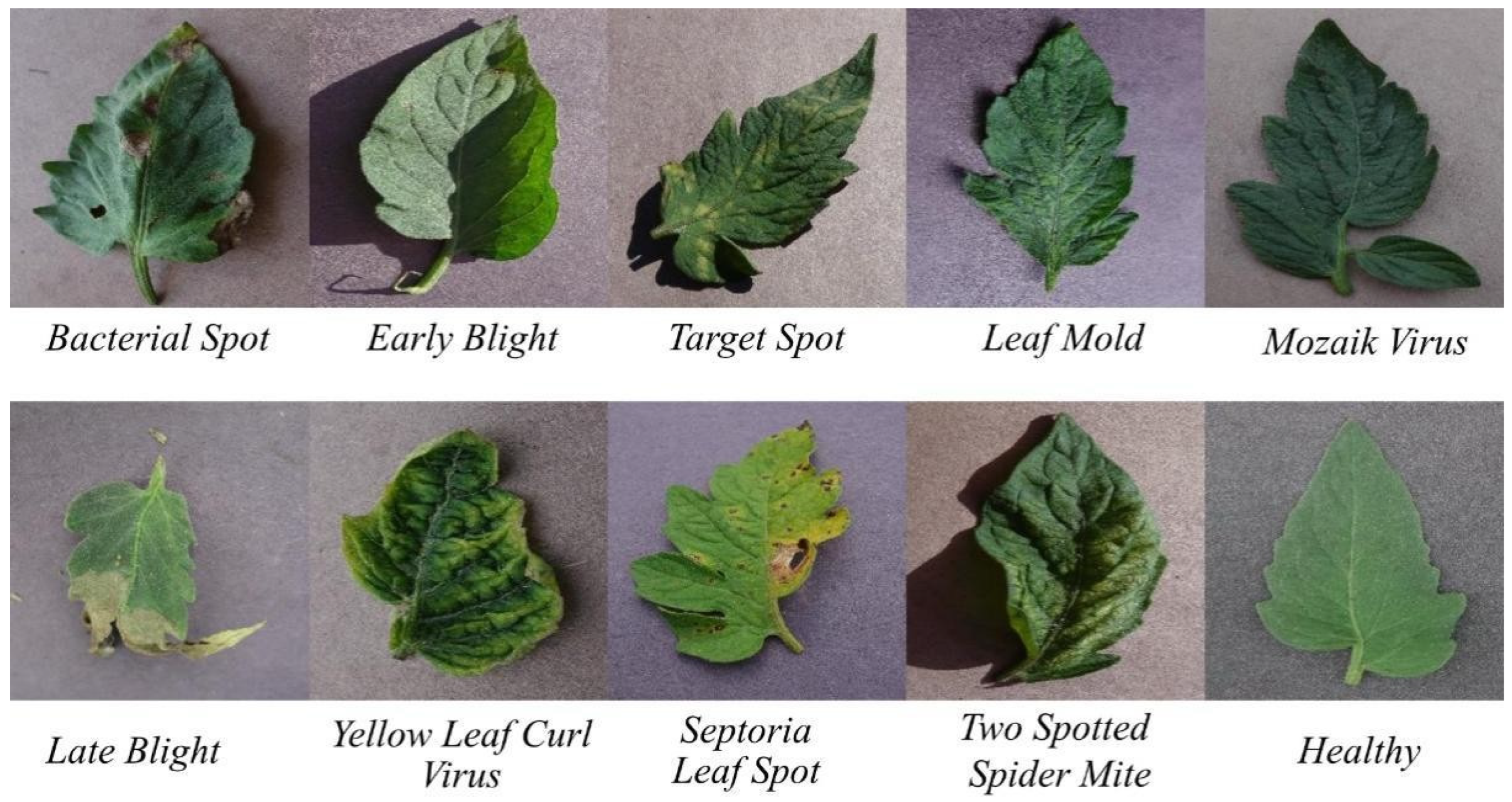
https://www.kaggle.com/datasets/kaustubhb999/tomatoleaf, accessed on 3 November 2022. There are 1000 types of images for each type of disease on tomato plant leaves. By taking 10 disease classes, data from 10,000 images were obtained. 
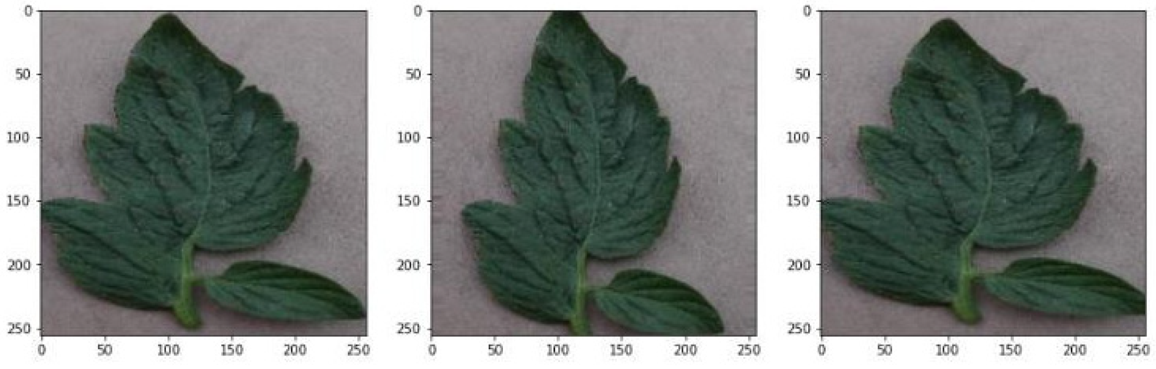
Figure 1 is a sample of each disease on tomato plant leaves. Each image’s dimensions are 256 by 256. Both the horizontal and vertical resolutions are 96 dpi. The bit depth is 24.

3.2. Image Preprocessing and Augmentation

Image preprocessing is a phase that prepares image data for subsequent processing [37]. This step must be completed in order for the data to run efficiently on the intended model. Image augmentation, meanwhile, is a method to increase the amount of data by altering the image’s shape, either by modifying the image’s rotation, position, or size [38]. Both phases of this research are mentioned below:
  • Rescale
Rescale is a preprocessing step that modifies the image’s size [39]. When the image is present in the application, it is represented by a value between 0 and 255. However, rescaling is conducted if the range of values is too large for the training procedure to be executed. The image value was divided by 255 so that it fell inside the range of 0 to 1.
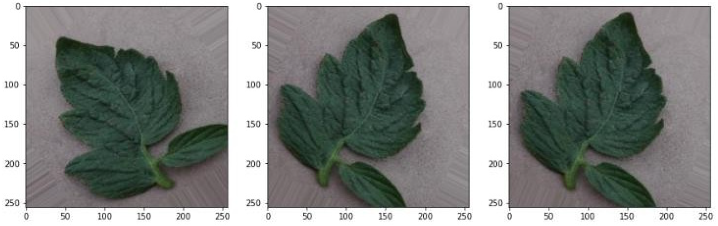
  • Rotation
As depicted in Figure 2, this is accomplished randomly by rotating the image clockwise a specified number of degrees between 0 and 90 degrees [40]. This research employed a rotation range of forty degrees.
  • Shift
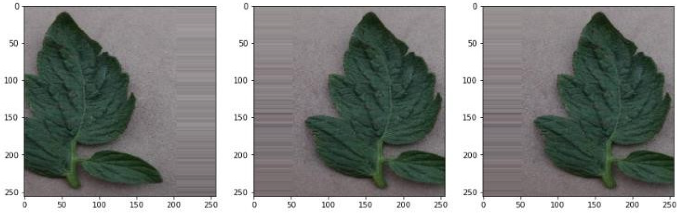
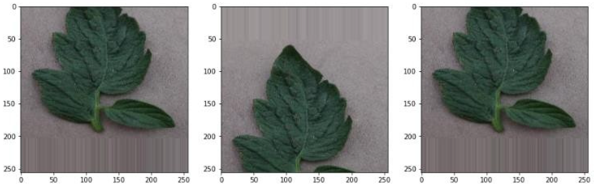
A shift is an enhancement technique for image movement [41]. It is performed to provide more varied picture data for image positions. There are two sorts of shift ranges: width and height. The height and breadth are respectively vertical and horizontal position shifts. Figure 3 and Figure 4 depict the implementations used in this investigation.
  • Zoom
Zoom is an augmentation technique for changing the size of an image [42]. It is intended that the image be more diverse in terms of size, as shown in Figure 5.

3.3. Data Splitting

Data splitting is the division of a dataset into multiple sections. In this study, the dataset was separated into training and testing data, where 10,000 training data and 1000 test data were used. The training data were used to develop the model, whilst the testing data were used to evaluate the model. In data training, data was also divided into 2 components, called data training and data validation. In order to conduct the validation, a 10-fold cross-validation technique was implemented.

3.4. Modeling

  • Hyperparameter
The objective of determining the proper hyperparameter is to create the ideal model. As indicated in Table 2, this study evaluated three types of hyperparameters, namely, the hidden layer, the trainable layer, and the dropout value of the layer.
  • Architecture
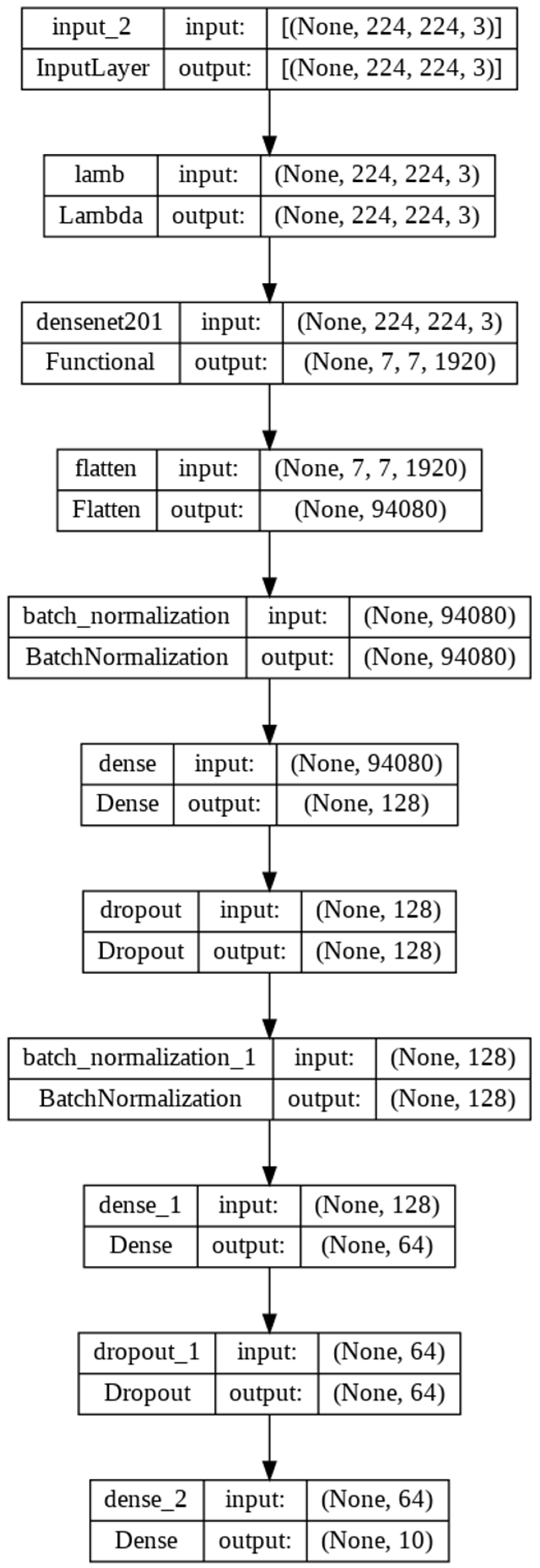
This study was constructed using Python and the Keras library. In Keras, the layers are defined progressively. The DenseNet layer, which was the initial layer, used an input value of 224 × 224. There were five levels of dense block. The first dense block layer received a 112 × 112 input and was convolved once. With a 56 × 56 input, the second dense block layer was convolved six times. With a 28 × 28 input, the third dense block layer was convolved twelve times. The fourth dense block layer was convolved 48 times with a 14 × 14 input, while the fifth dense block layer was convolved 32 times with a 7 × 7 input. The output was then applied to the flattened layer. The layer transformed data into 1-D vectors that could then be utilized by the fully connected layer. The subsequent step was to process the layer of batch normalization. This layer was used to standardize the data input. It could also accelerate the data training process and enhance the model’s performance. The following layer was the dropout layer, which was used to prevent overfitting. The dense layer comprised 10 units based on the number of classified classes. Prior to training, there were three configurations, including the loss function employing categorical cross-entropy and the Adam optimizer with a learning rate of 0.01. The structure can be seen in Figure 6.

3.5. Evaluation

This step evaluated the model using test data. It aimed to ensure that the model ran well. If the model did not display a good performance, then the model must be repaired. This study evaluated the model based on a confusion matrix, which showed how frequently correct and incorrect detections were made during classification. There were four possible permutations of predicted and actual values. The confusion matrix contained four columns labeled with the four possible outcomes of the classification process: true positive, true negative, false positive, and false negative. Accuracy, precision, recall, and F-1 scores can be calculated using these four factors. Accuracy describes how accurately the model can correctly classify. Therefore, accuracy is the ratio of correct predictions (positive and negative) to the entire set of data. In other words, accuracy is the degree of closeness of the predicted value to the actual value. Precision describes the level of accuracy between the requested data and the predicted results provided by the model. Thus, precision is defined as the ratio of the correct positive predictions to the overall positive predictions. Recall describes the success of the model in retrieving information. Thus, recall is the ratio of the correct positive predictions compared with all of the correct positive data. The F1-score is a combination of precision and recall.

3.6. Application

After locating the ideal model, the next stage was to develop an application for end users. The construction of the application utilized the Android platform and the Flutter application development framework. We incorporated the best model from the previous phase into the Android-based application. 
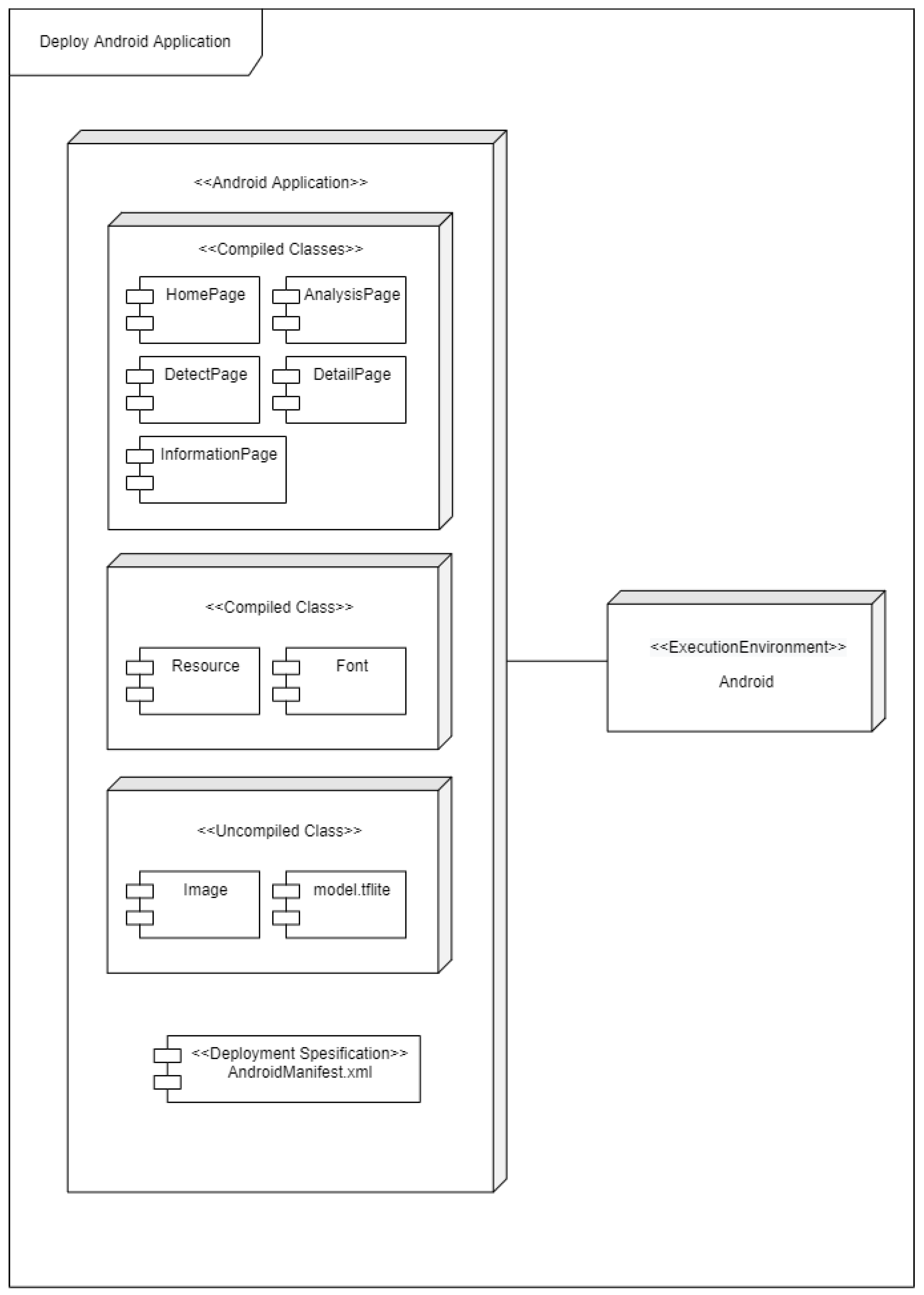
Figure 7 illustrates the deployment diagram. The Android program and the execution environment are the two nodes. There are four sections in the Android application section: compiled classes, compiled resources, uncompiled resources, and deployment specifications. This is the portion of the code that is run in the execution environment.

4. Results

4.1. Image Augmentation Analysis

In this experiment, image augmentation analysis was required to determine how the quantity of data impacted the correctness of the created model. Experiments were conducted by comparing the performance of the model with and without augmentation. As demonstrated in Table 3, experiments were conducted using constant hyperparameters. The hidden units indicate the required number of nodes for the hidden layer. This number falls between the number of input nodes and output nodes. Adam is an optimization technique that is an extension of stochastic gradient descent that has lately gained popularity in deep learning. This study employed the DenseNet algorithm, which is a transfer-learning technique. The epoch value was set to a low value so that the training procedure was not too lengthy. Table 4 displays the results of a comparison of the model’s performance with and without picture enhancement depending on the shift range, rotation range, and zoom range. The amount of data obtained with picture augmentation was 30,000, while it was only 10,000 without image augmentation. The model’s accuracy was only 85.32 percent without picture augmentation, compared with 92.53 percent with image augmentation. Due to the absence of variation in the training data, models without image augmentation earned lower scores and were therefore less competent at identifying image patterns. The experimental outcomes of this study are summarized in Table 5. The findings are described in Section 4.2, Section 4.3 and Section 4.4.

4.2. Analysis of the Number of Hidden Layers

This study examined whether the optimal model had two or three hidden layers. The model with two hidden layers contained 256 and 128 neurons, whereas the model with three hidden layers contained 256, 128, and 64 neurons. The results of the experiments utilizing 30 epochs and the Adam optimizer are presented in Table 5. They demonstrate that the number of hidden layers did not increase the accuracy of this study much. However, the addition of a concealed layer increased the running time. Using the hardware parameters of this investigation, it was determined that the best training time for a model with two hidden layers was less than eight hours on average. Three hidden layers required more than eight hours of instruction. Because memory use was directly proportional to the number of hidden layers. The addition of a hidden layer may also enhance the model’s potential for learning. It generated more intricate patterns that were useful for data prediction. However, a complicated pattern posed the risk of overfitting, in which the model predicts well on previously analyzed data but not on new data.

4.3. Trainable DenseNet Analysis

Analysis was based on the architectural layer that was retrained in DenseNet. On dense block 5 with 30 iterations and the Adam optimizer, two types of tests were conducted: without and with retraining (non-trainable layer). The trainable layer in dense block 5 led to greater precision than without it. The trainable system in dense block 5 achieved an average accuracy of 95%, whereas the model without a trainable layer achieved an average accuracy of 92%. It was due to the fact that the trainable layer retrained dense block 5. The repetition of training generated new weights, which, when added to the existing weights, could enhance the model’s optimization.

4.4. Dropout Analysis

The experiment altered the model’s dropout layer’s value. This study examined three dropout values: 0.2, 0.3, and 0.4. This dropout rate layer was positioned on a fully-connected layer with 30 iterations and an Adam optimizer. It indicated that a dropout rate of 0.4 had the best level of accuracy. It could also optimally manage overfitting. A dropout number that was too small resulted in a less ideal model for dealing with overfitting, while a dropout rate that was too high resulted in a less-than-optimal training process because too many neurons were deleted, i.e., it made the model’s categorization performance less optimal.

5. Discussion

After completing the trials on hyperparameters discussed in the preceding chapter, the research obtained values for these parameters that were deemed ideal. 
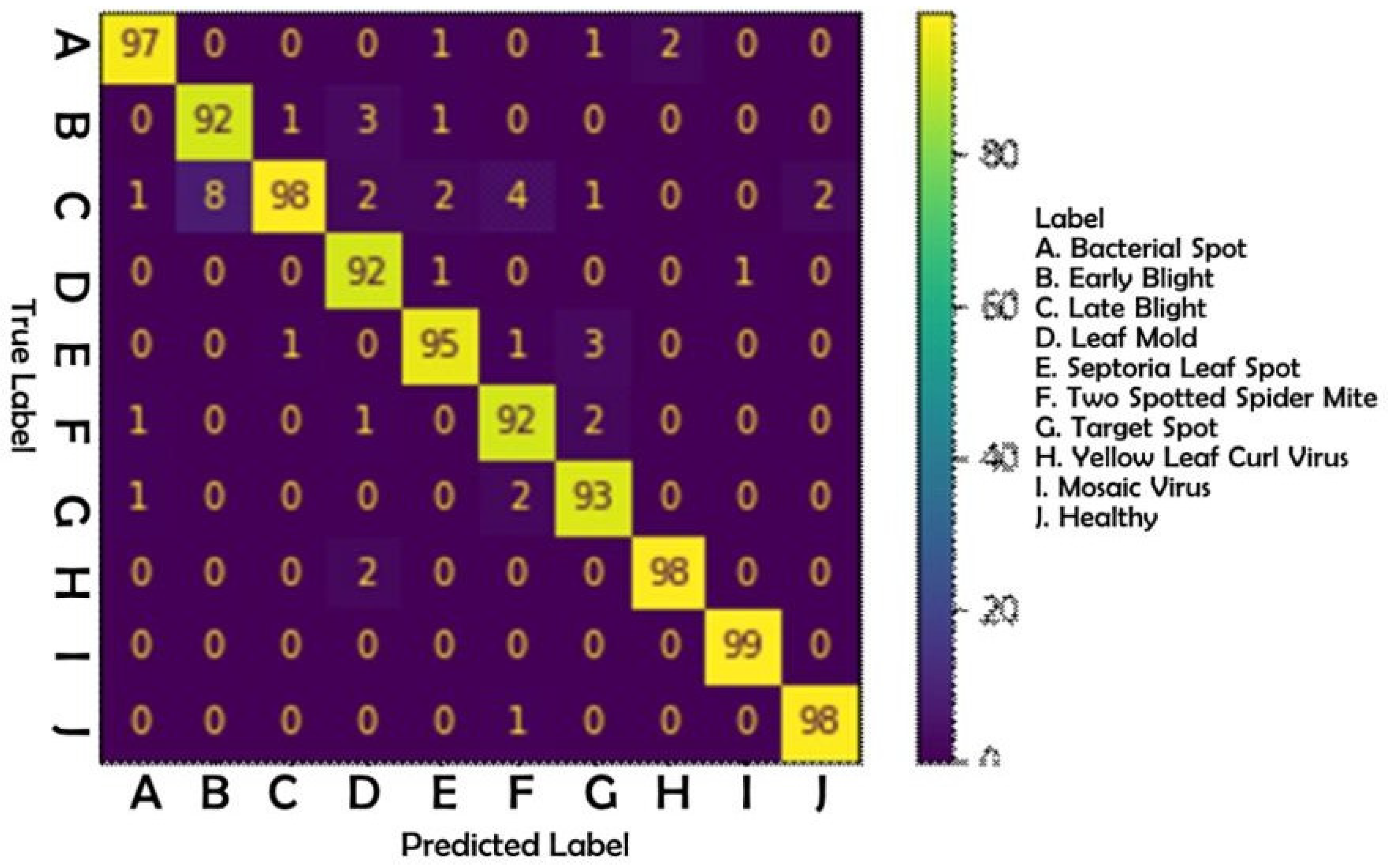
Table 6 gives the ideal hyperparameter values. The model was then evaluated using the test data that had been previously separated. As shown in Figure 8, the results of this test were produced in the form of a confusion matrix table. Following is an examination of Table 7:
  • Based on the precision value, it could be seen that mosaic virus disease received a score of 100 percent, whereas late blight disease received a score of 83 percent. The low precision value of late blight disease was caused by a high number of false positives. This occurred as a result of the detection of late blight disease in cases of other diseases. Based on the dataset at hand, the late blight illness possessed more diversified traits that resulted in misclassification.
  • According to the recall value, mosaic virus disease received the highest score of 99 percent, while two-spotted spider mite, leaf mold, and early blight disease received the lowest score of 92 percent. Due to a high percentage of false negatives on the label, the evaluation score for these three diseases was the lowest. This occurred due to detection errors, such as the misidentification of leaf mold illness as another disease. According to the data, two-spotted spider mites, leaf mold, and early blight likely resemble other diseases, particularly late blight.
  • The accuracy and F1-score in this study were 95.40% and 95.44%, respectively. With these values, along with the training, which had an accuracy of 95.79%, it can be concluded that the model had a good performance.
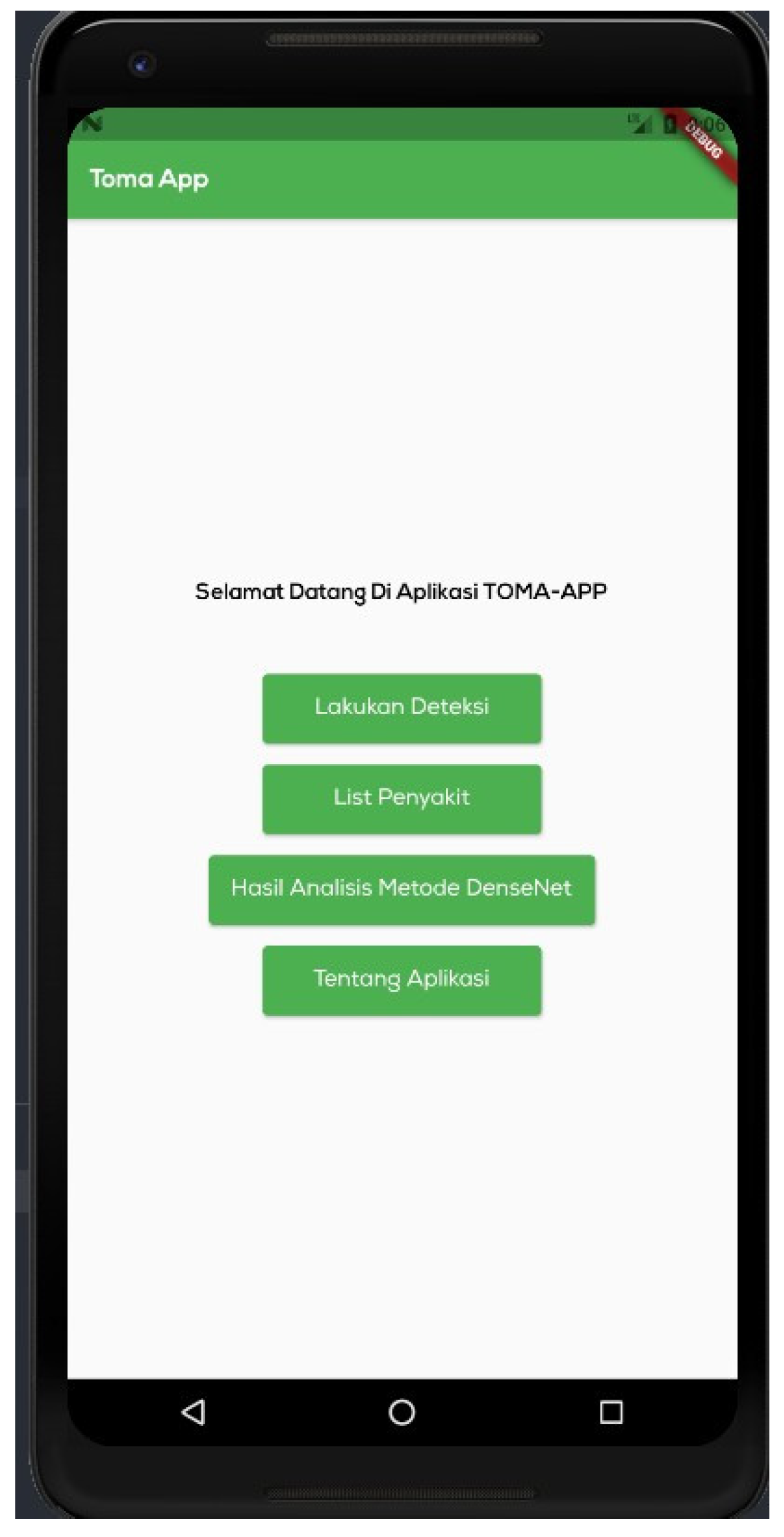
After identifying the optimal model, the authors of this study created an Android-based mobile application. The intended audience consisted of Indonesian farmers, hence the instructional language was Indonesian. Four primary menus make up the application: disease detection, disease list, analysis findings, and application description. Figure 9 depicts the home page.
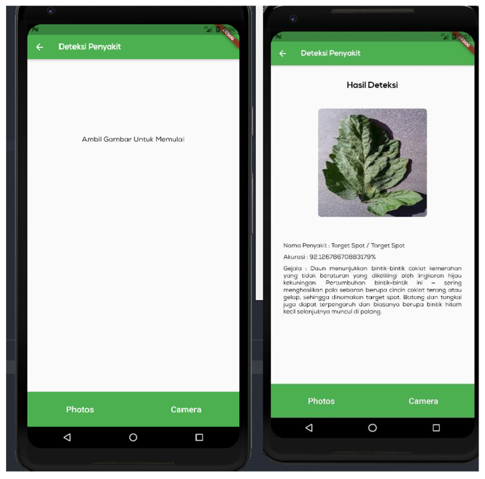
Figure 10 shows the ‘disease detection’ menu, which is a page for detecting illnesses on the leaves of tomato plants. On this page, the user will enter data to be processed by the DenseNet model. The model will detect the ailment that most closely corresponds to the visual input. There are two methods for importing photos: the camera and the gallery. 
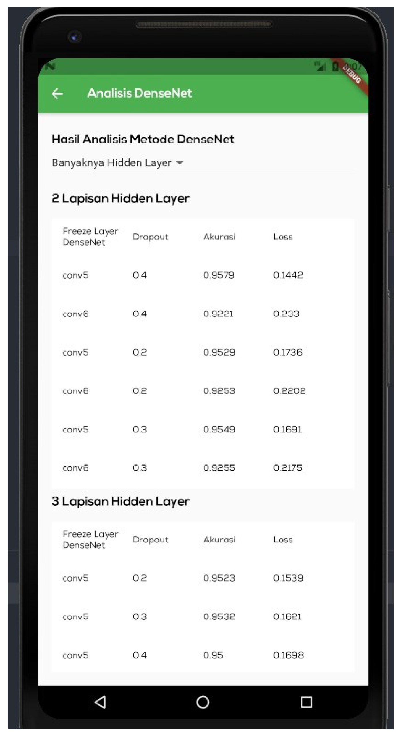
Figure 11 shows an ‘analysis results’ menu, which is the page displaying the outcomes of the conducted trials. This page contains a performance table of the model for each tested hyperparameter. Three hyperparameters, namely, the hidden layer, the dropout rate, and the trainable dense layer, are evaluated.

6. Conclusions

The following conclusions were made based on the research conducted on the classification of illnesses on tomato plant leaves and their implementation in mobile applications:
  • With two hidden layers, a dropout rate of 0.4, and the trainable layer in dense block 5, the best model of the DenseNet architecture was obtained. The model was constructed using 10-fold cross-validation to address local maximum issues.
  • An Android application for disease detection on tomato plant leaves was developed. The app’s primary function was disease detection. The technique consisted of capturing images to be forecasted based on the application’s stored model. This application is available in Indonesian for the convenience of Indonesian farmers.
  • Using DenseNet, the prediction of disease on tomato plant leaves performed admirably. The examination of the testing data using this model yielded accuracy and F1-score values of 95.4% and 95.4%, respectively.

Author Contributions

Conceptualization, I.N.Y.; methodology, I.N.Y. and A.H.; software, N.A.A.; validation, I.N.Y., N.A.A. and A.H.; formal analysis, I.N.Y.; investigation, I.N.Y. and N.A.A.; resources, N.A.A.; data curation, N.A.A.; writing—original draft preparation, I.N.Y.; writing—review and editing, I.N.Y.; visualization, N.A.A.; supervision, A.H.; project administration, I.N.Y.; funding acquisition, I.N.Y. All authors have read and agreed to the published version of the manuscript.

Funding

This study was funded by the Associate Professor Acceleration Research 2022, Universitas Padjadjaran, No. Contract: 2203/UN6.3.1/PT.00/2022.

Institutional Review Board Statement

Not applicable.

Informed Consent Statement

Not applicable.

Data Availability Statement

Not applicable.

Acknowledgments

The authors are grateful to the Rector, Directorate of Research and Community Service (DRPM), and Research Center for Artificial Intelligence and Big Data, Universitas Padjadjaran.

Conflicts of Interest

The authors declare no conflict of interest.

References

  1. Saptutyningsih, E.; Diswandi, D.; Jaung, W. Does social capital matter in climate change adaptation? A lesson from agricultural sector in Yogyakarta, Indonesia. Land Use Policy 2020, 95, 104189. [Google Scholar] [CrossRef]
  2. Wartenberg, A.C.; Blaser, W.J.; Roshetko, J.M.; Van Noordwijk, M.; Six, J. Soil fertility and Theobroma cacao growth and productivity under commonly intercropped shade-tree species in Sulawesi, Indonesia. Plant Soil 2020, 453, 87–104. [Google Scholar] [CrossRef]
  3. Sunarpi, H.; Kurnianingsih, R.; Ghazali, M.; Fanani, R.A.; Sunarwidhi, A.L.; Widyastuti, S.; Prasedya, E.S. Evidence for the presence of growth-promoting factors in Lombok Turbinaria murayana extract stimulating growth and yield of tomato plants (Lycopersicum esculentum Mill.). J. Plant Nutr. 2020, 43, 1813–1823. [Google Scholar] [CrossRef]
  4. Hidayatuloh, A.; Nursalman, M.; Nugraha, E. Identification of tomato plant diseases by Leaf image using squeezenet model. In Proceedings of the 2018 International Conference on Information Technology Systems and Innovation (ICITSI), Bandung, Indonesia, 22–26 October 2018. [Google Scholar]
  5. Yijo, S.; Asnawati, A.; Darma, S.; Achmad, G.N.; Arizandi, M.A.; Hidayati, T.; Darma, D.C. Social experiments on problems from tomato farmers during Covid-19-Indonesia case. SAR J. Sci. Res. 2021, 4, 7–13. [Google Scholar] [CrossRef]
  6. Mansur, A.; Ardi, R.P.; Mistriani, N. Optimizing the Preservation of Fresh Tomatoes into Tomato Dates to Increase the Shelf Life of Vegetable Food. Bp. Int. Res. Crit. Inst. (BIRCI-J.) Hum. Soc. Sci. 2021, 4, 9792–9803. [Google Scholar]
  7. Thwe, A.A.; Kasemsap, P.; Vercambre, G.; Gay, F.; Phattaralerphong, J.; Gautier, H. Impact of red and blue nets on physiological and morphological traits, fruit yield and quality of tomato (Solanum lycopersicum Mill.). Sci. Hortic. 2020, 264, 109185. [Google Scholar] [CrossRef]
  8. Tian, K.; Zeng, J.; Song, T.; Li, Z.; Evans, A.; Li, J. Tomato leaf diseases recognition based on deep convolutional neural networks. J. Agric. Eng. 2022. [Google Scholar] [CrossRef]
  9. Kaur, P.; Harnal, S.; Gautam, V.; Singh, M.P.; Singh, S.P. An approach for characterization of infected area in tomato leaf disease based on deep learning and object detection technique. Eng. Appl. Artif. Intell. 2022, 115, 105210. [Google Scholar] [CrossRef]
  10. Cui, S.; Ling, P.; Zhu, H.; Keener, H.M. Plant pest detection using an artificial nose system: A review. Sensors 2018, 18, 378. [Google Scholar] [CrossRef] [Green Version]
  11. Golhani, K.; Balasundram, S.K.; Vadamalai, G.; Pradhan, B. A review of neural networks in plant disease detection using hyperspectral data. Inf. Process. Agric. 2018, 5, 354–371. [Google Scholar] [CrossRef]
  12. Lu, T.; Han, B.; Chen, L.; Yu, F.; Xue, C. A generic intelligent tomato classification system for practical applications using DenseNet-201 with transfer learning. Sci. Rep. 2021, 11, 1–8. [Google Scholar] [CrossRef] [PubMed]
  13. Shewalkar, A. Performance evaluation of deep neural networks applied to speech recognition: RNN, LSTM and GRU. J. Artif. Intell. Soft Comput. Res. 2019, 9, 235–245. [Google Scholar] [CrossRef] [Green Version]
  14. Geetha, R.; Thilagam, T.; Padmavathy, T. Effective offline handwritten text recognition model based on a se-quence-to-sequence approach with CNN–RNN networks. Neural Comput. Appl. 2021, 33, 10923–10934. [Google Scholar] [CrossRef]
  15. Dua, N.; Singh, S.N.; Semwal, V.B. Multi-input CNN-GRU based human activity recognition using wearable sensors. Computing 2021, 103, 1461–1478. [Google Scholar] [CrossRef]
  16. Huan, R.H.; Shu, J.; Bao, S.L.; Liang, R.H.; Chen, P.; Chi, K.K. Video multimodal emotion recognition based on Bi-GRU and attention fusion. Multimedia Tools Appl. 2021, 80, 8213–8240. [Google Scholar] [CrossRef]
  17. Subramanian, B.; Olimov, B.; Naik, S.M.; Kim, S.; Park, K.H.; Kim, J. An integrated mediapipe-optimized GRU model for Indian sign language recognition. Sci. Rep. 2022, 12, 1–16. [Google Scholar] [CrossRef]
  18. Tang, J.; Shu, X.; Yan, R.; Zhang, L. Coherence constrained graph LSTM for group activity recognition. IEEE Trans. Pattern Anal. Mach. Intell. 2019, 44, 636–647. [Google Scholar] [CrossRef]
  19. Xing, X.; Li, Z.; Xu, T.; Shu, L.; Hu, B.; Xu, X. SAE+ LSTM: A New framework for emotion recognition from multi-channel EEG. Front. Neurorobot. 2019, 13, 37. [Google Scholar] [CrossRef] [Green Version]
  20. Li, R.; Liang, H.; Shi, Y.; Feng, F.; Wang, X. Dual-CNN: A Convolutional language decoder for paragraph image captioning. Neurocomputing 2020, 396, 92–101. [Google Scholar] [CrossRef]
  21. Kattenborn, T.; Leitloff, J.; Schiefer, F.; Hinz, S. Review on Convolutional Neural Networks (CNN) in vegetation remote sensing. ISPRS J. Photogramm. Remote Sens. 2021, 173, 24–49. [Google Scholar] [CrossRef]
  22. Yamashita, R.; Nishio, M.; Do, R.K.G.; Togashi, K. Convolutional neural networks: An overview and application in radiology. Insights Imaging 2018, 9, 611–629. [Google Scholar] [CrossRef] [PubMed] [Green Version]
  23. Nawaz, M.; Nazir, T.; Javed, A.; Masood, M.; Rashid, J.; Kim, J.; Hussain, A. A robust deep learning approach for tomato plant leaf disease localization and classification. Sci. Rep. 2022, 12, 1–18. [Google Scholar] [CrossRef] [PubMed]
  24. Guerrero-Ibañez, A.; Reyes-Muñoz, A. Monitoring Tomato Leaf Disease through Convolutional Neural Networks. Electronics 2023, 12, 229. [Google Scholar] [CrossRef]
  25. Chen, X.; Zhou, G.; Chen, A.; Yi, J.; Zhang, W.; Hu, Y. Identification of tomato leaf diseases based on combination of ABCK-BWTR and B-ARNet. Comput. Electron. Agric. 2020, 178, 105730. [Google Scholar] [CrossRef]
  26. Agarwal, M.; Gupta, S.K.; Biswas, K.K. Development of Efficient CNN model for Tomato crop disease identification. Sustain. Comput. Inform. Syst. 2020, 28, 100407. [Google Scholar] [CrossRef]
  27. Bhujel, A.; Kim, N.E.; Arulmozhi, E.; Basak, J.K.; Kim, H.T. A lightweight Attention-based convolutional neural networks for tomato leaf disease classification. Agriculture 2022, 12, 228. [Google Scholar] [CrossRef]
  28. Thangaraj, R.; Anandamurugan, S.; Kaliappan, V.K. Automated tomato leaf disease classification using transfer learning-based deep convolution neural network. J. Plant Dis. Prot. 2021, 128, 73–86. [Google Scholar] [CrossRef]
  29. Trivedi, N.K.; Gautam, V.; Anand, A.; Aljahdali, H.M.; Villar, S.G.; Anand, D.; Kadry, S. Early detection and classification of tomato leaf disease using high-performance deep neural network. Sensors 2021, 21, 7987. [Google Scholar] [CrossRef]
  30. Karthik, R.; Hariharan, M.; Anand, S.; Mathikshara, P.; Johnson, A.; Menaka, R. Attention embedded residual CNN for disease detection in tomato leaves. Appl. Soft Comput. 2020, 86, 105933. [Google Scholar]
  31. Chen, H.C.; Widodo, A.M.; Wisnujati, A.; Rahaman, M.; Lin, J.C.W.; Chen, L.; Weng, C.E. AlexNet convolutional neural network for disease detection and classification of tomato leaf. Electronics 2020, 11, 951. [Google Scholar] [CrossRef]
  32. Gonzalez-Huitron, V.; León-Borges, J.A.; Rodriguez-Mata, A.E.; Amabilis-Sosa, L.E.; Ramírez-Pereda, B.; Rodriguez, H. Disease detection in tomato leaves via CNN with lightweight architectures implemented in Raspberry Pi 4. Comput. Electron. Agric. 2021, 181, 105951. [Google Scholar] [CrossRef]
  33. Elhassouny, A.; Smarandache, F. Mobile application to recognize tomato leaf diseases using Convolutional Neural Networks. In Proceedings of the 2019 International Conference of Computer Science and Renewable Energies (ICCSRE), Agadir, Morocco, 22–24 July 2019. [Google Scholar]
  34. Ngugi, L.C.; Abdelwahab, M.; Abo-Zahhad, M. Tomato leaf segmentation algorithms for mobile phone applications using deep learning. Comput. Electron. Agric. 2020, 178, 105788. [Google Scholar] [CrossRef]
  35. Verma, S.; Chug, A.; Singh, A.P.; Sharma, S.; Rajvanshi, P. Deep learning-based mobile application for plant disease diagnosis: A proof of concept with a case study on tomato plant. In Applications of Image Processing and Soft Computing Systems in Agriculture; IGI Global: Hershey, PA, USA, 2019; pp. 242–271. [Google Scholar]
  36. Kim, J.; Kim, J. The impact of imbalanced training data on machine learning for author name disambiguation. Scientometrics 2018, 117, 511–526. [Google Scholar] [CrossRef] [Green Version]
  37. Maier, A.; Syben, C.; Lasser, T.; Riess, C. A gentle introduction to deep learning in medical image processing. Z. für Med. Phys. 2019, 29, 86–101. [Google Scholar] [CrossRef]
  38. Bloice, M.D.; Roth, P.M.; Holzinger, A. Biomedical image augmentation using Augmentor. Bioinformatics 2019, 35, 4522–4524. [Google Scholar] [CrossRef] [PubMed]
  39. Xiao, M.; Zheng, S.; Liu, C.; Wang, Y.; He, D.; Ke, G.; Liu, T.Y. Invertible image rescaling. In European Conference on Computer Vision; Springer: Cham, Switzerland, 2010. [Google Scholar]
  40. Khalifa, N.E.; Loey, M.; Mirjalili, S. A comprehensive survey of recent trends in deep learning for digital images augmentation. Artif. Intell. Rev. 2021, 55, 1–27. [Google Scholar] [CrossRef]
  41. Nanni, L.; Maguolo, G.; Paci, M. Data augmentation approaches for improving animal audio classification. Ecol. Inform. 2020, 57, 101084. [Google Scholar] [CrossRef] [Green Version]
  42. Sánchez-Peralta, L.F.; Picón, A.; Sánchez-Margallo, F.M.; Pagador, J.B. Unravelling the effect of data augmentation transformations in polyp segmentation. Int. J. Comput. Assist. Radiol. Surg. 2020, 15, 1975–1988. [Google Scholar] [CrossRef]
Figure 1. Examples of tomato plant leaves.
Computation 11 00020 g001
Figure 2. Rotation illustration.
Computation 11 00020 g002
Figure 3. Illustration of width shift.
Computation 11 00020 g003
Figure 4. Illustration of height shift.
Computation 11 00020 g004
Figure 5. Illustration of zoom.
Computation 11 00020 g005
Figure 6. Network architecture.
Computation 11 00020 g006
Figure 7. Design of the mobile application.
Computation 11 00020 g007
Figure 8. Confusion matrix.
Computation 11 00020 g008
Figure 9. Main menu. This presentation is in Indonesian. The display comprises four menus: “Lakukan Deteksi” to detect diseases of tomato plant leaves, “List Penyakit” containing a list of diseases, “Hasil Analisis Metode Densenet” to load the findings of densenet method analysis, and “Tentang Aplikasi” containing information about the application.
Computation 11 00020 g009
Figure 10. Disease detection implementation page. The page is given in Indonesian. This menu is for identifying tomato plant leaf diseases. On this page, the user will upload images that will be utilized by the constructed model. The image on the left demonstrates that there are two ways to upload photos: using the camera and the gallery. The image on the right displays the results of the detection.
Computation 11 00020 g010
Figure 11. Experimental results implementation page. This page displays the outcomes of experiments that have been conducted. This page is formatted as a table listing every tested hyperparameter. Three hyperparameters, namely the hidden layer, the dropout rate, and the trainable dense layer, are evaluated.
Computation 11 00020 g011
Table 1. Some applications of deep learning in daily life.
ArchitectureApplication
RNNSpeech recognition [12], handwriting recognition [13], activity recognition [14]
GRUSpeech recognition [12], emotion recognition [15], sign language recognition [16]
LSTMSpeech recognition [12], activity recognition [17], emotion recognition [18]
CNNHandwriting recognition [13], activity recognition [14], image captioning [19], remote sensing [20]
Table 2. Hyperparameters.
HyperparameterValue
Trainable layer[Non-trainable, trainable]
Dropout[0.2, 0.3, 0.4]
Number of dense layers[2, 3]
Table 3. Hyperparameter values in the image augmentation analysis.
HyperparameterValue
Hidden units128
OptimizerAdam
Epoch30
Batch size32
Table 4. Image augmentation analysis.
DatasetAccuracy (%)
With image augmentation92.53
Without image augmentation85.32
Table 5. Experimental results.
Hidden LayersDropoutTrainable LayerAccuracy (%)Loss (%)Running Time (h)
20.2Non-trainable92.5322.028.02
20.3Non-trainable92.5521.758.52
20.4Non-trainable92.2123.38.78
20.2Dense block 595.2917.367.48
20.3Dense block 595.4916.917.56
20.4Dense block 595.7914.427.82
30.2Non-trainable92.2124.699.31
30.3Non-trainable92.2826.089.55
30.4Non-trainable92.8728.3110.02
30.2Dense block 595.2315.398.42
30.3Dense block 595.3216.218.85
Table 6. The optimal hyperparameters.
HyperparameterValue
Trainable layerTrainable layer on dense block 5
Dropout0.4
Number of dense layers2
Table 7. Evaluation of each class.
LabelPrecision (%)Recall (%)F1-Score (%)
Bacterial spot96.0397.0096.51
Early blight94.8492.0093.40
Late blight83.0598.0089.90
Leaf mold97.8792.0094.84
Septoria leaf spot95.0095.0095.00
Two-spotted spider mite95.8392.0093.87
Target spot96.8793.0094.89
Yellow leaf curl virus98.0098.0098.00
Mosaic virus100.0099.0099.49
Healthy98.9898.0098.49
Macro average95.6595.4095.44
Accuracy95.40
Disclaimer/Publisher’s Note: The statements, opinions and data contained in all publications are solely those of the individual author(s) and contributor(s) and not of MDPI and/or the editor(s). MDPI and/or the editor(s) disclaim responsibility for any injury to people or property resulting from any ideas, methods, instructions or products referred to in the content.

