Enhancing Algorithm Selection through Comprehensive Performance Evaluation: Statistical Analysis of Stochastic Algorithms

Abstract

Analyzing stochastic algorithms for comprehensive performance and comparison across diverse contexts is essential. By evaluating and adjusting algorithm effectiveness across a wide spectrum of test functions, including both classical benchmarks and CEC-C06 2019 conference functions, distinct patterns of performance emerge. In specific situations, underscoring the importance of choosing algorithms contextually. Additionally, researchers have encountered a critical issue by employing a statistical model randomly to determine significance values without conducting other studies to select a specific model for evaluating performance outcomes. To address this concern, this study employs rigorous statistical testing to underscore substantial performance variations between pairs of algorithms, thereby emphasizing the pivotal role of statistical significance in comparative analysis. It also yields valuable insights into the suitability of algorithms for various optimization challenges, providing professionals with information to make informed decisions. This is achieved by pinpointing algorithm pairs with favorable statistical distributions, facilitating practical algorithm selection. The study encompasses multiple nonparametric statistical hypothesis models, such as the Wilcoxon rank-sum test, single-factor analysis, and two-factor ANOVA tests. This thorough evaluation enhances our grasp of algorithm performance across various evaluation criteria. Notably, the research addresses discrepancies in previous statistical test findings in algorithm comparisons, enhancing result reliability in the later research. The results proved that there are differences in significance results, as seen in examples like Leo versus the FDO, the DA versus the WOA, and so on. It highlights the need to tailor test models to specific scenarios, as p-value outcomes differ among various tests within the same algorithm pair.

1. Introduction

In the realms of mathematics and computer science, optimization problems involve the quest for the finest solution among all possible valid options. The ultimate goal is to secure the most exceptional outcome, known as the global optimal solution. Nevertheless, when confronted with a problem featuring multiple optimal points, the existing techniques have primarily focused on unearthing the best solution that prevails across numerous local optima. These local optima represent solutions superior to their immediate neighbors, yet fall short of achieving the overall paramount solution.

In situations where the values of these local solutions closely resemble each other, a circumstance can arise where two algorithms exhibit seemingly indistinguishable performances. However, a nuanced disparity emerges: one algorithm disperses its solutions widely throughout the search space, while the other algorithm bunches them together in proximity [1]. There exist instances when it becomes pivotal to accentuate these distinctions by employing a comparative analysis between the two algorithms, employing statistical methodologies to ascertain the concurrences between them. This evaluation involves scrutinizing the disparities through diverse statistical models, encompassing nonparametric approaches, to comprehensively gauge the variations [2].

In the ever-expanding landscape of optimization algorithms, benchmarks play a crucial role with a two-fold purpose. They not only validate the performance of novel algorithms but also enable head-to-head evaluations among various algorithms. These benchmarks have effectively demonstrated the prowess of optimization algorithms, employing fundamental statistical indicators like mean, standard deviation, and median for comparison [3]. Moreover, supplementary methods, like benchmarks and performance profiles, have been harnessed to achieve this goal [4,5]. Notably, contemporary research papers focusing on benchmark comparisons increasingly incorporate frequentist statistical approaches, such as null-hypothesis testing, marking a prominent trend in the field.

Numerous meta-heuristic stochastic optimization algorithms have emerged, highlighting the necessity to thoroughly assess the efficacy of any novel algorithm. This evaluation and adjustment are indispensable for facilitating a meaningful comparison against the performance of cutting-edge algorithms [6]. Simultaneously, under multiple studies, the process of benchmarking assumes pivotal importance, as it lays the foundation for identifying the optimal algorithm. However, securing a high-quality benchmark remains a formidable challenge. The preliminary phase of the benchmarking theory involves delineating the problem domain, an intricate task due to the requisite “uniform” distribution of test functions across the entire expanse of potential functions within the problem domain [7].

Presently, within the evolutionary algorithms’ domain [8], a considerable number of published papers have substantiated benchmarks through statistical experimental evaluations, performed for each test function encompassed by the benchmark in several single-objective or multiobjective optimization algorithms [9,10,11]. Following the selection of the suite of benchmark functions, the benchmarking outcomes rely on performance metrics and statistical ranking methodologies, as highlighted. The role of meticulous statistical analyses is paramount, as they furnish the foundational data upon which conclusions are drawn. Conventionally, one widely adopted approach involves utilizing statistical tests for comparative purposes, hinging on the values of acquired solutions (such as fitness function values or test function outcomes, as elucidated in subsequent points). This approach is in harmony with the idea of hypothesis testing, although it occasionally neglects the distribution of obtained solutions throughout the exploration space, and it can also be influenced by compiler optimization settings over time [12].

Lately, a majority of optimization algorithms aimed at achieving superior quality and performance rely on test functions for assessing and distinguishing their effectiveness. In the present day, there are two primary categories of test functions extensively utilized. Firstly, the classical benchmark test functions encompass a collection of nineteen functions, which are classified into three distinct categories: unimodal, multimodal, and composite [13]. The second category involves ten functions, referred to as the CEC-C06 2019 conference functions [14], specifically employed to evaluate and adjust the efficacy of newly proposed algorithms. These functions continue to be extensively adjusted within modern benchmark collections. To validate their efficacy, it becomes imperative to establish a comparative framework among various result groups. This involves employing both parametric and nonparametric statistical tests to discern any hypothetical agreements between them. Notably, the nonparametric variant of the two-sample t-test, which fulfils specific assumptions, forms a key part of this comprehensive study’s discussions.

Adhering to the concept of hypothesis testing, there has been a lack of attention directed towards the distribution of acquired solutions within the exploration space [15]. Insights regarding the distribution of solutions in the search space can be harnessed in various manners. Users might seek an optimization algorithm capable of yielding either widely dispersed or closely clustered solutions based on their preferences. Moreover, this distribution information can illuminate the relative merits and drawbacks of the algorithms being compared. In theory, this study can offer valuable contributions by enabling a comprehensive evaluation of solutions based on their values and their spatial arrangement within search algorithms that were previously employed. This study has centered its perspectives on the following significant facets that constitute its proposed contributions:

• The p-value tests reveal significant performance disparities between algorithm pairs, highlighting statistical significance in the comparisons. The algorithms being compared also display statistical significance in terms of the values of their achieved solutions and their distribution. Thus, this study compares algorithms that exhibit similar abilities in both exploration and exploitation;
• Analyzing algorithm performance across a range of test functions, including classical benchmarks and CEC-C06 2019 conference functions, reveals varying effectiveness, with certain algorithms demonstrating superiority in specific contexts;
• The study assesses algorithms across various test functions to understand their suitability for different optimization challenges and seeks to identify algorithm pairs with favorable statistical distributions;
• The study investigates multiple nonparametric statistical hypothesis models, such as the Wilcoxon rank-sum test, single-factor, and two-factor analyses, to gain insights into algorithm performance across diverse evaluation criteria, improving our overall understanding of their capabilities;
• Identifying inaccuracies in previous statistical test results during algorithm comparisons, thoroughly investigating these discrepancies, and integrating the rectification process;
• The results offer valuable guidance in choosing appropriate algorithms, highlighting their proven performance in various scenarios. This supports professionals in making informed decisions when statistically evaluating algorithm pairs.

The primary objective of this paper is to demonstrate the impact of test functions on the performance of optimization algorithms through the application of various statistical hypothesis tests. Additionally, the paper aims to assess the degree of success in yielding high-quality results within the proposed functions. These statistical tests are employed both for single-objective and multiobjective algorithms. Significantly, the core emphasis of this intricate investigation is centered on the diversities within the statistical model, rather than delving into the particulars of the utilized algorithm types and the approach with which they are implemented. On the flip side, the endeavor intends to provide valuable guidance to developers of artificial intelligence, aiding them in the selection of the most suitable hypothesis model. This contribution is especially pertinent when considering the common perplexity experienced by numerous researchers who find themselves in the position of wanting to undertake a statistical comparison between their freshly proposed algorithm and established conventional algorithms. Also, this study advocates for parametric or nonparametric statistical tests due to their flexibility with insignificant sample sizes. The rejection of the null hypothesis in these tests does not pinpoint specific differences among compared algorithms but signals general distinctions among result samples. A special session on real-parameter optimization illustrates test application on renowned evolutionary and swarm intelligence algorithms. Concluding evaluations offer considerations and recommendations for practitioners, demonstrated in a comprehensive case study with seven algorithms over benchmark functions. The study extends to important issues regarding test behavior and applicability, emphasizing selecting the most suitable test based on circumstances and comparison type [16,17].

The subsequent sections of this paper are organized as follows: Section 2 initiates by delving into related background work studies, elucidating previous engagements with metaheuristic algorithms, and highlighting the techniques employed for statistical result assessment. Section 3 focuses on the process of choosing a reference algorithm based on performance evaluation. In Section 4, a comprehensive exploration of the statistical models used for comparing algorithm pairs is presented. Section 5 encompasses the outcomes and the experimental evaluation through a series of tables. The discussion and method evaluation or adjustment take center stage in Section 6. Ultimately, Section 7 concludes and summarizes the work, while also proposing avenues for future research endeavors.

2. Related Works

Exploring and dissecting optimization algorithms using performance measures constitutes a pivotal realm of inquiry within the domain of evolutionary computation. This facet takes on even greater significance when considering the intricate area of single- or multi (many)-objective optimization [18]. These experimental evaluations ought to encompass observed calculations and make common errors, blending statistical analyses and hypothesis conjectures, all synchronized with evaluation functions adhering to established standards and iterative processes [19]. The participants in this experimental work would ideally be consistent and represented by the same cohort of search agents or entities.

Yet, the lack of fitting benchmark challenges remains noticeable across various sectors of evolutionary computation research. The act of delving into statistical evaluation brings to light a noticeable scarcity, encompassing more than just numerical variety. It extends to encompass issues of accessibility, user-friendliness, and the ability to distinctly outline the traits of benchmark functions. The prevailing benchmarks underpinning extant algorithms each lay claim to their distinctive standards, orchestrating a harmonious pursuit of optimization outcomes [20]. These statistical benchmark-birthed revelations spotlight the efficacy of algorithms, like the genetic algorithm (GA) [21], dragonfly algorithm (DA) [10], particle swarm optimization (PSO) [22], and differential evolution (DE) [23], etching a testimony to their operational prowess.

The landscape is rife with bewilderment when it comes to employing a statistical underpinning for hypotheses within metaheuristic algorithms to unearth p-values. To illustrate, consider the likes of the Mirjalili and Lewis algorithm (2016) as applied to the whale optimization algorithm (WOA) [24]. These algorithms, when scrutinized, did not engage in the statistical evaluation of hypothesis values in comparison with other algorithms. Rather, they contented themselves with the customary statistical evaluation methods, such as averages and standard deviations. Conversely, the slime mould algorithm (SMA) unfurls a distinct approach [25]. It shed light on the true skill statistic (TSS) residing within the domain of combined pairwise comparisons [26]. This methodology surfaced as a means to pit literature-based algorithms against each other. To ascertain this, reliance was placed on the outcomes derived from the iterative version and the function evaluation version of the Friedman test. Expanding on this approach, the scope widened to include the multiobjective fitness-dependent optimizer (MOFDO) [27]. Within this context, the Friedman test once again played a central and indispensable role in extracting meaningful statistical values. It is worth highlighting that the Wilcoxon sum-rank test model provided substantial reinforcement to this intricate analytical expedition. Furthermore, a significant creative influence can be observed in the utilization of two distinct sets of function benchmarks and the incorporation of three distinct types of statistical significance models to assess the performance of the newly proposed optimization algorithms.

Table 1. Literature and the categorization of several existing dependent-work algorithms.

Algorithm	Litreature Year	Problem Types	Statistical Model	Referncing
Differential Evolution	2005	Single	Statistical standards	[23]
Whale Optimization	2016	Both	Wilcoxon sum-rank	[24]
Slime Mould	2020	Single	Wilcoxon sum-rank	[25]
Fitness-Dependent Optimizer	2019	Both	ANOVA single-factor and Friedman test	[9,27]
Golden Eagle Optimization	2021	Single	Wilcoxon sum-rank and statistical standards	[28,29]
Moth–flame Optimization	2015	Both	Wilcoxon sum rank	[30,31]
Learner-Performance-based Behavior	2021	Single	ANOVA single-factor	[32]
Leo	2023	Single	Wilcoxon sum-rank	[11]
FOX	2023	Single	ANOVA single-factor	[33]
Salp Swarm Algorithm	2017	Both	Wilcoxon sum-rank	[34]

showcases specific studies that shed light on the findings gleaned from prior research, and also classifies the type of problem of algorithms into “single” as a single-objective algorithm and “both” as single- and multiobjective algorithm. Nevertheless, it is important to note that numerous algorithms have been developed and statistically assessed.

To find the best knowledge in the discourse adjacent to evolutionary algorithms, there appears to be a dearth of dedicated publications that exclusively center on the statistical association of stochastic optimization algorithms. This comparison pertains to the stochastic and hypothetical attributes of the outcomes derived within the search space. Previous works have demonstrated a lack of a systematic approach in addressing the statistical issues outlined in Table 1. Additionally, the deficiency is evident in various proposed optimization algorithms and has prompted an examination of these limitations. Specifically, the absence of a standardized criterion for selecting the appropriate statistical model to assess significance and performance is a focal point of this investigation. Nonetheless, this aspect holds significant importance, as it plays a critical role in acquiring insights into the exploratory capabilities of the compared algorithms. This reliance is contingent on the two group benchmarks previously mentioned, and it has the potential to offer a more profound conception of the methodologies employed to enhance the comparative statistical power of exploration between the algorithms. Particularly, within the domain of the single-objective, learner-performance-based behavior (LPB) algorithm [32], a statistical evaluation or adjustment was assumed, encompassing the LPB algorithm with the literature algorithms. The effort involved deriving p-values grounded in the ANOVA single-factor test model [35], even though the authors referenced to the Wilcoxon sum-rank test model [36]. It is pertinent to mention that an error in decision-making was observed in the case of the single-objective FDO in statistical evaluation [9]. This delusion was rectified upon meticulous review and accurate result verification. In a similar vein, the FOX algorithm [33] emerges as an outlier, as the computation of the p-value was executed through a statistical approach. However, it is worth noting that no particular test model was explicitly referenced in this context.

Lagrange elementary optimization (Leo) [11] and salp swarm algorithm (SSA) [34] algorithms have been instrumental in extracting noteworthy p-values via the Wilcoxon rank-sum test, applied to assess hypothesis-comparison outcomes. The outcomes, coupled with their respective analyses and the discoveries unveiled within specific subsections, converge to bestow upon these algorithms the promising potential to tackle real-world conundrums set within enigmatic search spaces. Finally, when navigating the intricate tapestry of authentic search spaces, the whereabouts of the coveted global optimum remain tantalizingly concealed. This conundrum underscores the paramount importance of orchestrating a symphony of exploration and exploitation in perfect harmony. This delicate equilibrium is what markedly heightens the probability of stumbling upon the global optimum, a testament firmly rooted in the realm of hypothetical outcomes. After identifying limitations in various proposed algorithms and drawing insights from comparative case studies in the literature, we selected different algorithms based on their respective strengths and weaknesses.

3. Evaluating Performance for the Selection of the Reference Algorithm

In discussing algorithm selection and identifying common issues, the challenge arises from the propagation of algorithms tailored to specific, stringent criteria. Nevertheless, some overarching criteria have emerged. To address this, benchmarks need to evaluate both functional and nonfunctional requirements to gauge their fulfilment. Furthermore, specific conditions, like a large problem set or an odd number of problems, should be considered to facilitate statistical tests and mitigate potential issues in comparative analysis, such as cycle ranking or the survival of the nonfittest paradoxes [37,38].

The experimental benchmark comprises synthetic functions designed to challenge optimization algorithms. It should encompass a variety of functions with diverse characteristics, including varying local optima, shifting global optima, rotated coordinate systems, nonseparable components, noise, and multiple problem sizes, tailored to the expected problem complexities. Additionally, when addressing novel real-world problems, authors must thoughtfully curate or generate suitable instances for evaluation, which is common when tackling uncharted areas in real environments [39].

Selecting reference algorithms for comparison is a critical consideration, closely tied to the previous guideline. Firstly, when the proposed algorithm builds upon basic algorithms, it is crucial to include them in the comparison to assess each one’s individual impact. Secondly, after choosing the benchmark, it is essential to incorporate the best-performing methods for that specific benchmark into the evaluation. Regrettably, many papers overlook this step, failing to compare their proposed algorithm against competitive alternatives. In a well-informed experiment, at a minimum, the best-performing algorithms in the benchmark’s domain should be included. Furthermore, it is important to evaluate similar algorithms, not just within the same algorithm family (e.g., PSO-based or GA-based), but also related inspired-based algorithms or improvements on previous methods [38,40]. Thus, it is our contention that solely comparing new methods to outdated classic algorithms, which have clearly been surpassed, should be avoided. Participating new algorithms in benchmarks is crucial to address concerns about the scientific contribution of the proposal. However, discussing the computational method and intricate looping formulas in detail is challenging due to the computational complexity inherent in each algorithm, including complex mathematical problems. Based on these measurements, we briefly outline the computational complexity considerations, considering the merits and drawbacks of the selected algorithms for this statistical comparison study, as detailed below:

▪

The primary algorithm, DA, is often gradient descent, a common first-order optimization approach. DA employs particle-based exploration, like PSO, by initializing dragonfly positions and step vectors within variable-defined ranges using random values. It combines simplicity with elements of the stochastic gradient descent, adaptive learning rate, and conjugate gradient methods. However, DA can be sensitive to randomness and may not always converge [41];

▪

WOA utilizes a multistrategy approach, combining mathematical formulations and loop structures, as demonstrated in a specific case study which was influenced by the hunting behaviors of humpback whales. Its advantages include effective strategies like prey search, prey encirclement, and spiral bubble-net movements. However, it may be computationally expensive and lacks a guarantee of reaching the global optimum [42];

▪

SSA, the other algorithm of choice, exhibits resemblances to other swarm-based optimization methods, like PSO and ACO, particularly in terms of collective intelligence and exploration–exploitation mechanisms with mathematical looping. SSA is beneficial for locating optimal points, demonstrating versatility, and enhancing global exploration capability and convergence speed. However, it is prone to issues such as vulnerability to schedules, occasional entrapment in local optima, and sensitivity to mutation and crossover strategies [34];

▪

FDO improves individual positions by adding velocity to their current locations, drawing from PSO principles and also influenced by bees’ swarming behavior and collaborative decision-making. However, FDO’s drawback lies in limited exploration, slow convergence, and sensitivity to proposal distribution [43];

▪

LPB enhances computational complexity for high school graduates’ university transition and study behaviors using genetic algorithm operators. It is versatile and adaptable to different optimization tasks and problem domains, making it a versatile choice. However, LPB has limited exploration, slow convergence, and sensitivity to proposal distribution [44];

▪

Leo uses a GA and a novel Lagrangian operator to find the optimal immune system postvaccination, excelling in robust combinatorial optimization for real-world applications. However, it may require extensive tuning and its convergence depends on the choice of the combiner operator [11,45];

▪

The FOX algorithm is inspired by the hunting strategies of real foxes, employing distance measurement techniques for efficient prey pursuit. It is ideal for optimizing costly to evaluate functions with simplicity and efficiency. However, it can become computationally expensive and necessitates a careful choice of priors [33].

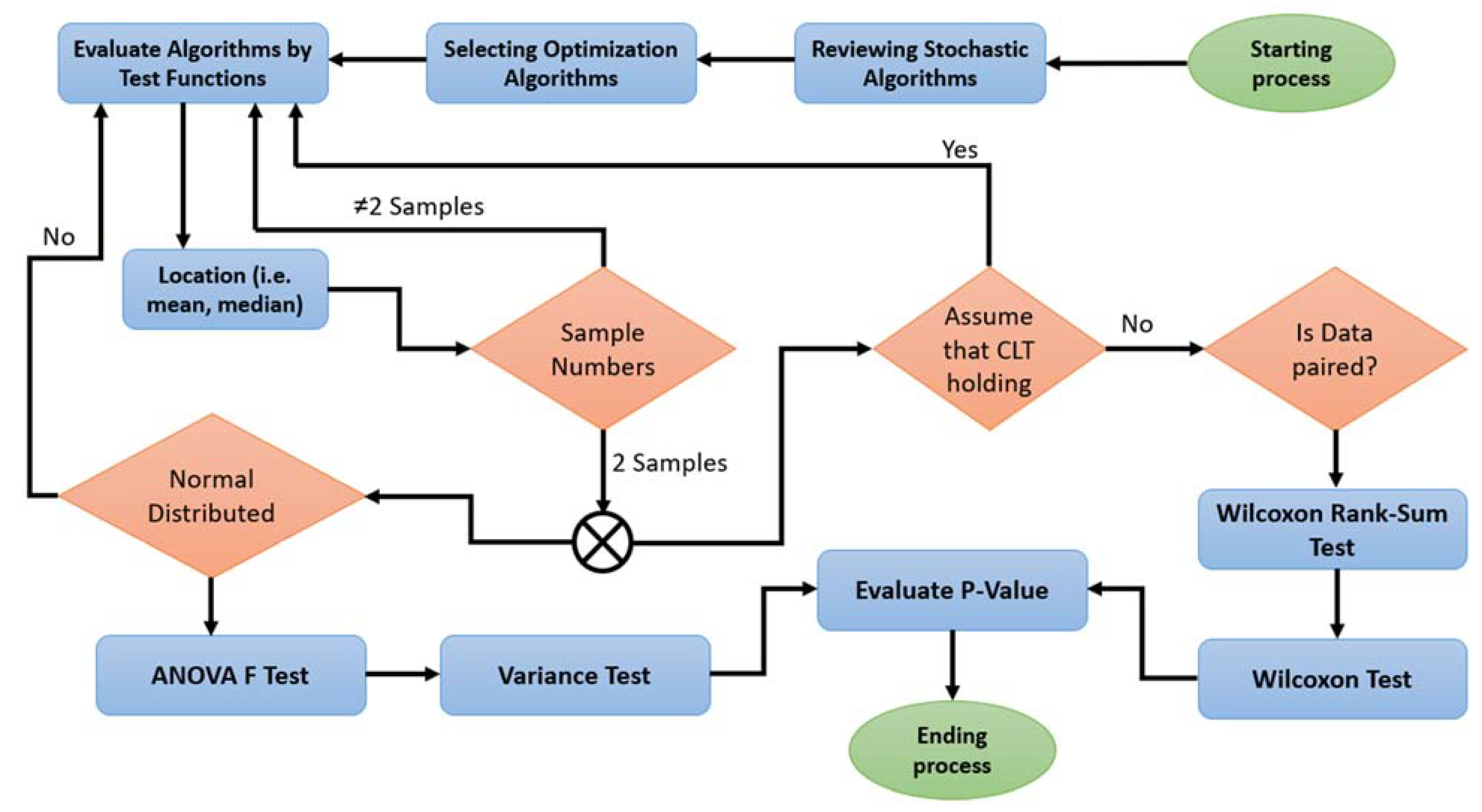
4. Methodological Framework for Extended Statistical Comparisons

The significance of the method’s usefulness is central in the domain of evaluating metaheuristic algorithms. It harnesses the strength of p-values obtained from benchmark datasets. In this process, the method serves as a connection between processed global or optimal data and meaningful discoveries, offering a statistical viewpoint that allows for a thorough examination of the effectiveness of various metaheuristic algorithms. By focusing on p-values derived from the benchmark dataset between two algorithms as a nonparametric variable, the benefit method contributes to a robust framework for comparing and contrasting the efficacy of different metaheuristic algorithms. This approach holds the potential to shed light on the relative strengths and weaknesses of algorithms, enabling practitioners to make informed decisions about which strategies are better suited for specific problem domains or optimization scenarios. Furthermore, employing p-values as an evaluation metric adds objectivity and quantifiability, particularly for stochastic algorithms with variables [46]. This approach offers a standardized measure that enhances the rigor and evidence-based nature of algorithmic evaluation and adjustment. Consequently, the benefit method becomes a valuable tool in advancing metaheuristic optimization, promoting innovation, and propelling the development of more efficient algorithms.

Typically, statistical comparison operates effectively with one-dimensional data and is not suitable for comparing distributions of acquired solutions in either the search space or for high-dimensional data. To address this limitation, a hypothetical test comes to the aid, extending the depth of statistical comparison by employing multiple hypothetical tests. This approach calculates p-values from these tests, enabling comparisons between stochastic tests. Each test produces distinct outcomes, which is why researchers observe the selection of the statistical model in this process during experimental evaluation [47]. In this study, an assessment has been conducted on all the test functions within the chosen benchmark groups. The evaluation necessitates the selection of a sequence of time points after the discovery of the global solution, spanning across extensive iterations.

With a specific goal, the process involves identifying the optimal global value through a predetermined iteration count. This aims to achieve a balanced and equitable reputation for various types of test functions within the classical benchmark test functions group and the CEC-C06 2019 conference functions for several stochastic algorithms. These selected stochastic algorithms will be further discussed in the subsequent sections. The outcomes of the test functions are then juxtaposed across the algorithms using statistical-hypothesis-testing models, such as the Wilcoxon rank-sum test, the single-factor ANOVA table [35], and the two-factor ANOVA table [48]. To delve deeper into the method’s mechanics, the procedural steps can be accurately observed in Figure 1, which effectively illustrates the evaluation process. Based on the central limit theorem (CLT) [49], the distribution of sample means tends to resemble a normal distribution as the sample size increases, irrespective of the underlying population distribution. Typically, sample sizes of 30 or more are deemed adequate for the CLT to apply. Consequently, the p-values obtained through these three statistical models in this study are influenced by this principle. The innovation unveiled in this methodology has relied on the sequential dance of the following steps:

▪

Initiating the quest by delving into the article, unraveling solutions to the problem;

▪

Choosing from the array of contemporary and renowned stochastic optimization algorithms;

▪

Subjecting each algorithm to a rigorous evaluation, involving 30 times for each test function, to unearth the ultimate optimal solution;

▪

Unveiling the statistical gems within, such as the illustrious mean, the steadfast median, and more, as they illuminate the path to standard solutions;

▪

To determine the sample size for each pair of samples with respect to the chosen test function and pair of algorithms, the following should be showcased:

˗

When dealing with a sample that does not conform to CLT and lacks balanced data, it is advisable to subject it to the influential Wilkson rank-sum test. If it does not pass, a reconsideration of the evaluation will be necessary;

˗

For a sample that exhibits normal distributions, it should be scrutinized with the influential ANOVA F test, involving a thorough examination of variances.

▪

Concluding the computation, the influence of p-values will be instrumental in appraising all test functions in alignment with the pair of algorithms. This will determine the algorithms’ performance and suitability for the task at hand.

Figure 1. The proposed statistical methodology for delineating the data analysis process.

Figure 1. The proposed statistical methodology for delineating the data analysis process.

4.1. Wilkson Rank-Sum Test

The assumptions for comparing the means of two sample populations using the T-test include independent samples, equal variance, and a normal distribution. If these conditions are not met, an alternative is the Wilcoxon rank-sum test. This alternative only requires the first two assumptions—sample independence and similar variance—without specifying a particular data distribution. The Wilcoxon rank-sum test, also known as the Mann–Whitney U test if the data sample does not pair, compares independent samples [50]. Meanwhile, the Wilcoxon signed-rank test compares related or matched samples. It is useful for paired difference tests on a single sample to assess differences in population mean ranks when the sample is no more than thirty individuals. The Wilcoxon rank-sum test is a nonparametric approach to comparing independent samples and identifying distribution differences.

Accordingly, these nonparametric tests do not assume the normal distribution of samples. The Wilcoxon unpaired two-sample test statistic is akin to the technique proposed by Gustav Deuchler in 1914, although Deuchler erred in calculating the variance. In 1945, Wilcoxon introduced a significance test with a point null hypothesis and its complementary alternative. However, this paper only presented the null hypothesis for equal sample sizes and contained limited tabulated points (though larger tables were provided in a subsequent paper). A comprehensive analysis of the statistics was conducted by Henry Mann and Donald Ransom Whitney in their 1947 paper. This is why the Wilcoxon rank-sum test is also referred to as the Wilcoxon–Mann–Whitney test, and the Mann–Whitney U test is equivalent to the Wilcoxon rank-sum test [51,52].

Furthermore, the Wilcoxon rank-sum test is applied in the microbiome study to compare differences in median values of alpha-diversity measures, proportions of core genera, and the abundance of specific genera for categorical variables and matched samples, respectively. Particularly when the sample size (N) is no more than thirty, a common approach is to convert data points into their respective ranked values—where rank one or a positive rank corresponds to the smallest value, rank two or a negative rank to the next smallest value, and so on [36].

The resulting p-value from this test aids in evaluating and adjusting the null hypothesis, which posits that two samples or more originated from populations with identical distributions [53]. Below is a step-by-step breakdown of how to calculate the p-value using the Wilcoxon rank-sum test according to [54,55]:

• Hypothesis formulation: The hypotheses encompass the null hypothesis ($H_0$), indicating that the two samples originate from populations with the same distribution, and the alternative hypothesis ($H_1$), implying that the two samples arise from populations with distinct distributions.
• Combining and ranking data: Begin by consolidating the two samples into a unified dataset. Proceed to assign ranks to the combined data, arranging them in ascending order, irrespective of their source sample. In the case of tied values, allocate the average rank to these tied values.
• Calculating rank sums: Compute the sum of ranks for each sample. Denote the sum of ranks for sample one as $R_1$ and for sample two as $R_2$.
• Calculating the test statistic (U): In this pivotal stage, our attention is captivated by the intricate calculation of the test statistic (U). This calculation takes into account the smaller rank sum and the sample sizes associated with it. However, it is important to note that this process is subject to specific conditions and limitations. The calculation U depends on the comparison of two rank sums, $R_1$ and $R_2$, which correspond to the two groups being compared using the rank-sum ($R_1$ or $R_2$) method, as we have assessed two algorithms in this study. The computation of U is illustrated by Equation (1) and as follows:

  $${\mathit{U}=\mathit{U}}_{\mathit{R}1 \mathit{o}\mathit{r} \mathit{R}2}={(\mathit{n}}_1\times {\mathit{n}}_2)+\frac{{\mathit{n}}_1 \mathit{o}\mathit{r} {\mathit{n}}_2\left({\mathit{n}}_1 \mathit{o}\mathit{r} {\mathit{n}}_2+1\right)}{2}-R_1 \mathrm{or} R_2$$

  (1)

  where $n_1 \mathrm{o}\mathrm{r} n_2$ represent the number of data points in each respective sample; in our study, each sample consists of 30 data-observation points.
  Then:
  If $R_1$ is the smaller rank sum, then U is equal to $U_{R1}$.
  If $R_2$ is the smaller rank sum, then U is equal to $U_{R2}$.
• Calculating the expected value and variance of U: During this stage, you should compute the expected value $\left(E\left(U\right) or {\mu }_u\right)$ and variance $\left(Var\left(U\right) or {\mathsf{\sigma }}_u\right)$ of the test statistic $U$ by employing the formula specific to the Wilcoxon rank-sum test.
• Calculating the $\mathit{Z}-\mathit{s}\mathit{c}\mathit{o}\mathit{r}\mathit{e}$: Determine the Z-score utilizing Formula (2). Subsequently, compute the expected value $\left({\mu }_u\right)$ using Equation (3), and find the variance $\left({\mathsf{\sigma }}_u\right)$ by using Equation (4).

  $$\mathit{Z}=\frac{\mathit{U}-{\mathit{\mu }}_{\mathit{u}}}{{\mathsf{\sigma }}_u}$$

  (2)

  where

  $${\mathit{\mu }}_{\mathit{u}}=\frac{({\mathit{n}}_1\times {\mathit{n}}_2)}{2}$$

  (3)

  $${\mathsf{\sigma }}_u=\sqrt{\frac{{\mathit{n}}_1\times {\mathit{n}}_2\times ({\mathit{n}}_1+{\mathit{n}}_2+1)}{12}}$$

  (4)
• Calculating the p-value and making a decision: For a two-tailed test, which involves comparing distributions for differences in both directions, calculate the p-value using the standard normal distribution linked to the absolute value of the calculated $Z-score$ (where $Z_{abs}$ represents the $Z-score$). Furthermore, in the context of a one-tailed test, where the aim is to compare distributions for differences in a specific direction, compute the p-value by referring to the relevant tail of the standard normal distribution as assessed through Formula (5).

  $$\mathit{p}-\mathit{v}\mathit{a}\mathit{l}\mathit{u}\mathit{e}=2\times \mathbf{m}\mathbf{i}\mathbf{n}\left(\mathit{P}\left(\mathit{Z}>{\mathit{Z}}_{\mathit{a}\mathit{b}\mathit{s}}\right),\mathit{P}\left(\mathit{Z}<{\mathit{Z}}_{\mathit{a}\mathit{b}\mathit{s}}\right)\right)$$

  (5)

For making a decision, compare the computed p-value to the predetermined significance level (alpha). This step helps determine whether to reject the null hypothesis. If the calculated p-value is equal to or less than the alpha value, you have grounds to reject the null hypothesis in favor of the alternative hypothesis.

4.2. Single-Factor ANOVA Table

A single-factor is part of a one-way layout, characterized by a factor with multiple levels and numerous observations within each level. This arrangement facilitates the computation of observation averages within each level of the factor. The residuals provide insights into the variability present within these levels. Furthermore, the mean can be computed for each level and then combined to establish a comprehensive grand mean. From this, we can delve into the disparities between the signal-level means and the grand mean to comprehend the implications of different levels. Ultimately, by comparing the variability within levels to that spanning across levels, the term “analysis of variance (ANOVA)” comes to fruition.

ANOVA is employed to ascertain if the means of two or more distinct groups are equivalent. ANOVA utilizes the null hypothesis ($H_0$)) and an alternative hypothesis ($H_1$), similar to the Wilcoxon rank-sum test. In a one-factor ANOVA table, the p-value is computed using the F-distribution. As such, the ANOVA test is employed to assess mean disparities among various groups, aiming to establish whether noteworthy statistical differences exist between those group means. Expressing all of this in Equation (6) form is a straightforward process.

$${\mathit{Y}}_{\mathit{i}\mathit{j}}=\mathit{\mu }+{\mathit{\alpha }}_{\mathit{i}}+{\mathit{ϵ}}_{\mathit{i}\mathit{j}}$$

(6)

$Y_{ij}$ signifies an observation within a group indexed by $i$ and a specific observation within that group indexed by $j$. The $j\mathrm{t}\mathrm{h}$ data point according to Equation (6) within level $i$ is a composite of three fundamental elements: the common value (grand mean), the level effect (deviation from the grand mean), and the residual (remaining variance); $\mu$ denotes the overall or grand mean of all observations; ${\alpha }_i$ stands for the effect related to the $i\mathrm{t}\mathrm{h}$ group (level), representing the difference between the overall mean μ and the mean of group $i$. Lastly, ${ϵ}_{ij}$ indicates the residual or error term for the $j\mathrm{t}\mathrm{h}$ observation, capturing unexplained variation resulting from factors not considered in the model, including random noise and uncontrollable influences on observations.

Primary methods for estimating the one-way layout values can be presented as summarized in

Table 2. Enforcing consistency in statistical analysis through ANOVA table regulation [48].

Source of Variation	The Sum of Squares (SS)	Degree of Freedom (DF)	Mean Square (MS)	$\mathit{F}-\mathit{S}\mathit{t}\mathit{a}\mathit{t}\mathit{i}\mathit{s}\mathit{t}\mathit{i}\mathit{c}$
Factor (F) (Treatments)	${SSF=\sum n_j\left({\overline{Y}}_j-{\overline{Y}}_{ij}\right)}^2$	$K-1$	$MSF=\frac{SSF}{k-1}$	$\frac{MSF}{MSE}$
Residual (E) (Error)	$SSE=\sum \sum {\left(Y_{ij}-{\overline{Y}}_j\right)}^2$	$N-K$	$MSE=\frac{SSE}{N-k}$
Corr. Total	$SST=\sum \sum {\left(Y_{ij}-{\overline{Y}}_{ij}\right)}^2$	$N-1$

, depicted below, depending on [56,57]. Subsequent tests can then be conducted to establish the significance of the factor levels. The ANOVA table dissects the variance components in the data, differentiating between the treatment-based variance and the error or residual variance. ANOVA tables are also commonly generated by statistical computing software as a standard outcome for ANOVA analysis.

In the context of this scenario, the symbol ${\overline{Y}}_j$ denotes the average value observed in the $j\mathrm{t}\mathrm{h}$ treatment or group, as defined in Formula (7). Similarly, ${\overline{Y}}_{ij}$ represents the overall average value across all treatments, as expressed in Formula (8). In these equations, $K$ corresponds to the count of treatments or distinct comparison groups, while $N$ represents the total number of observations or the overall size of the sample.

$${\overline{Y}}_j=\frac{1}{K} \sum _{i=1}^K{Y}_{ij}$$

(7)

$${\overline{Y}}_{ij}=\frac{1}{NK} \sum _{i=1}^K\sum _{j=1}^N{Y}_{ij}$$

(8)

The p-value in a one-factor ANOVA table is computed based on the F-statistic, as illustrated in

Table 3. Unimodal benchmark functions statistical comparison of Leo with the FDO, LBP, and DA.

TFs	p-Value Tests	Leo vs. FDO	Leo vs. LPB	Leo vs. DA
TF1	Wilcoxon rank-sum test	0.000002	0.000031	0.000031
	Single-factor	5.78 × 10−2	7.72 × 10−6	5.78 × 10−2
	Two-factor	6.27 × 10−2	3.24 × 10−5	6.27 × 10−2
TF2	Wilcoxon rank-sum test	0.047162	0.000002	0.000002
	Single-factor	6.48 × 10−2	1.09581 × 10−10	3.08665 × 10−6
	Two-factor	1.16 × 10−1	1.16757 × 10−8	1.60543 × 10−5
TF3	Wilcoxon rank-sum test	0.002585	0.000002	0.000002
	Single-factor	1.02 × 10−1	5.52049 × 10−9	1.67 × 10−1
	Two-factor	1.00 × 10−1	1.65436 × 10−7	1.72 × 10−1
TF4	Wilcoxon rank-sum test	0.000002	0.000002	0.000031
	Single-factor	9.49 × 10−8	8.74288 × 10−23	3.22 × 10−1
	Two-factor	1.20 × 10−6	7.61671 × 10−16	3.26 × 10−1
TF5	Wilcoxon rank-sum test	0.557743	0.781264	0.000148
	Single-factor	5.18 × 10−2	2.03 × 10−1	4.50 × 10−2
	Two-factor	6.28 × 10−2	2.30 × 10−1	5.14 × 10−2
TF6	Wilcoxon rank-sum test	0.000002	0.000002	0.057096
	Single-factor	7.00 × 10−5	1.83 × 10−4	3.16 × 10−1
	Two-factor	1.84 × 10−4	4.02 × 10−4	3.21 × 10−1
TF7	Wilcoxon rank-sum test	0.000002	0.000097	0.000002
	Single-factor	3.48738 × 10−14	1.06251 × 10−5	5.30 × 10−3
	Two-factor	7.24577 × 10−11	5.96148 × 10−5	6.98 × 10−3

Bold values indicate no statistical significance at p < 0.05.

. The ANOVA test serves the purpose of comparing means among several groups, aiming to ascertain whether notable statistical distinctions exist between the averages of these respective groups. In addition, the overarching Equation (9), used to compute the p-value within a one-factor ANOVA table, involves the F-observed value, which is contingent upon the observed F-statistic in the ANOVA table. The expression (F-statistic > F-observed) denotes the likelihood of attaining an F-statistic exceeding the observed F-observed value under the null hypothesis.

$$p-value=P\left(F-statistic>F-observed\right)$$

(9)

Calculating the p-value entails the following procedural steps:

• Determining the degrees of freedom: First, one crucial step involves determining the degrees of freedom for both the numerator, which signifies the between-group variability, and the denominator, which signifies the within-group variability, of the F-statistic. This process is elaborated upon in Figure 2.
• Employing the observed F-statistic: Next, utilize the observed F-statistic alongside the degrees-of-freedom values. You can then either consult an F-distribution table or employ statistical software to precisely calculate the p-value.
• Comparison with the significance level: Finally, compare the calculated p-value with a selected significance level (alpha), often set at α = 0.05. This comparison determines if the obtained outcome holds statistical significance. Should the p-value be lower than the significance level, the null hypothesis is rejected.

It is noteworthy that various statistical software packages (such as R v.4.3.0, SPSS v.27, and Python v.3.11.1, with libraries like scipy or statsmodels, among others) are capable of automatically performing these calculations during ANOVA analyses. Thus, manual calculations are generally unnecessary, unless you aim to gain a comprehensive understanding of the underlying procedures.

4.3. Two-Factor ANOVA Table

A two-factor ANOVA, also referred to as a two-way ANOVA, extends the scope of a one-way ANOVA by examining how two distinct independent categorical variables impact a continuous dependent variable. The primary distinction between a one-way ANOVA and a two-way ANOVA pertains to the number of independent variables under scrutiny and their interactions. In the context of a two-way ANOVA, the examination encompasses the influence of two independent variables on a dependent variable. Moreover, this analytical approach assesses the effect of these independent variables on the anticipated outcome and their interrelation with the outcome itself. The distinction between random and systematic factors rests upon their statistical impact within a dataset, with systematic factors being deemed statistically significant while random factors lack such influence.

In a two-way ANOVA, two independent categorical variables (factors) exert an influence on the dependent variable. This method examines the primary effects of each factor and also considers potential interactions between these factors. It goes beyond merely identifying differences in group means and delves into how these differences might be influenced by combinations of the two factors. The ANOVA table designed for a two-way ANOVA encompasses distinct sources of variation corresponding to each main effect and their interactions. This table also includes vital statistical measures, such as degrees of freedom, sum of squares, mean squares, the F-statistic, and the p-value. Additionally, the interaction term within the context of a two-way ANOVA signifies whether the impact of one factor on the dependent variable is contingent upon the specific level of the other factor. This interaction term provides insight into how the combined effects of the two factors contribute to the overall outcome.

The sole disparity between two-factor ANOVA and single-factor ANOVA lies in the approach to computation. The divergence emerges in the sequence of calculations: initially, calculate the sum of squares factor A (SSa) to assess the squared deviations attributed to variations in factor A. Subsequently, calculate the sum of squares factor B (SSb) to quantify the squared deviations stemming from variations in factor B. Following this, calculate the sum of squares interaction (SSi) to determine the squared differences resultant from the interplay between factor A and factor B. Importantly, it should be acknowledged that these sources of variation in the two-factor ANOVA table are calculated and presented in the same manner as observed in the single-factor ANOVA table, as explained in the earlier subsection.

Consequently, the determination of the degrees of freedom becomes imperative to establish the suitable degrees of freedom for each source of variation (A, B, interaction, error). The concluding step entails the calculation of p-values, specifically selecting p-values aligned with each F-statistic through reference to the F-observed in the F-distribution table [58]. This signifies that the process of generating an ANOVA table in a two-way ANOVA possesses heightened intricacy due to the incorporation of multiple factors and their interactions.

5. Result and Statistical Analysis

The outcome determination based on the methodology has been established. Initially, a variety of stochastic algorithms are chosen to assess statistical outcomes and their concurrence. It is worth noting that each algorithm was employed to verify the accuracy of the proposed algorithm. To gauge the efficacy of this algorithm, multiple common benchmark functions from the existing literature were employed. Algorithms for making selections in diverse scenarios are categorized based on the strategies employed in automatic parameter tuning. These strategies are then further organized into three distinct tiers: the straightforward generate–evaluate methods, the iterative generate–evaluate methods, and the advanced high-level generate–evaluate methods [59].

In the pursuit of optimization, various parameters are carefully chosen, guided by the principles of evolutionary inspiration. The process of parameter tuning becomes a delicate tightrope act, aiming to strike the perfect equilibrium between avoiding underfitting and guarding against overfitting. Yet, many of these studies fall short in substantiating how they maintain the vital balance between exploration and exploitation. It is insufficient merely to assert that the first algorithm surpasses the second in maintaining this balance; such claims necessitate empirical scrutiny to establish their validity. Some approaches achieve this equilibrium by employing evolutionary operators explicitly designed to enhance it, like crossover and mutation operators. Meanwhile, different algorithms investigate how authors gauge the exploration and exploitation balance, often relying on indirect measures, such as convergence towards optimal solutions, diversity, and tangibility of the solutions [38,60].

Moreover, some algorithms put forth a classification of techniques aimed at fostering population diversity. Authors aspiring to incorporate this analysis into their research endeavors must undertake a quantitative experimental investigation to substantiate their assertions [38]. In consideration of the background of this research field and the pursuit of global algorithmic excellence, it is challenging to identify innovative standards for the determination of testing rounds and the process of iterative exploration. Depending on the most recent algorithms we have employed in this study, which collectively established a consensus, we have prescribed the utilization of 30 rounds as a universally accepted approach, involving 500 successive iterations to attain a global point in each round, employing an ensemble of 80 search agents.

These evaluations and adjustment errors are carried out under conditions where sample distributions are either equal to or less than 30, and where assumptions are roughly equivalent or symmetric. However, it is important to note that the criteria for spread variance and normalcy are not entirely met. This approach is adopted since, in real-world scenarios, achieving precise solutions holds more significance than the time taken. Moreover, the adaptability of algorithms allows for refinement and repeated testing by virtually anyone, indicating that clients prioritize the effectiveness of an algorithm over its execution time. In this research, the outcomes of all algorithms, as assessed by the test functions, are meticulously analyzed to reveal substantial nonparametric relationships. These results are categorized into two groups: one based on classical benchmarks and the other on the CEC-C06 2019 benchmark test functions.

5.1. Statistical Assessment of Classical Benchmark Test Functions

In this phase of evaluation, the algorithms are categorized based on their effectiveness and innovative nature. The initial category pertains to the Leo algorithm, which is compared against the FDO, LPB, and DA in terms of agreement. Following this, the DA is compared against FDO and LPB. This is done to establish a rationale for comparison. It is noteworthy that many initial optimization algorithms, predominantly those rooted in inspired optimization or population-based optimization, have been previously contrasted with the DA. Conspicuously, classical benchmarks are distinctly classified across three tabulated sets, as appraised in the subsequent subsections. These sets encompass a selection of three types of test functions: unimodal, multimodal, and composite. These test functions are segregated into these three categories, each designed with the intent of assessing the algorithm’s efficiency and its alignment with specific benchmark perspectives.

5.1.1. Unimodal Benchmark Test Functions

In a thorough examination of Leo’s impact alongside the FDO, LPB, and DA, utilizing a set of unimodal benchmark functions, several noteworthy findings come to light. As outlined in

Table 4. Unimodal benchmark functions for the statistical comparison of the DA with FDO and LBP.

TFs	p-Value Tests	DA vs. FDO	DA vs. LBP
TF1	Wilcoxon rank-sum test	4.32 × 10−8	0.000002
	Single-factor	3.10 × 10−1	7.72 × 10−6
	Two-factor	3.14 × 10−1	3.23997 × 10−5
TF2	Wilcoxon rank-sum test	0.000002	0.000002
	Single-factor	6.47 × 10−2	1.07 × 10−10
	Two-factor	6.98 × 10−2	1.16 × 10−8
TF3	Wilcoxon rank-sum test	0.000002	0.000002
	Single-factor	8.72 × 10−2	5.52 × 10−9
	Two-factor	9.25 × 10−2	1.65 × 10−7
TF4	Wilcoxon rank-sum test	0.000031	0.000031
	Single-factor	3.21 × 10−1	3.42 × 10−6
	Two-factor	3.26 × 10−1	4.25684 × 10−5
TF5	Wilcoxon rank-sum test	0.005667	0.002765
	Single-factor	4.04 × 10−3	6.74 × 10−3
	Two-factor	5.94 × 10−3	1.05 × 10−2
TF6	Wilcoxon rank-sum test	0.323358	0.000031
	Single-factor	3.16 × 10−1	7.53 × 10−1
	Two-factor	3.21 × 10−1	7.63 × 10−1
TF7	Wilcoxon rank-sum test	0.000002	0.000002
	Single-factor	3.17 × 10−14	7.77 × 10−13
	Two-factor	6.69 × 10−11	5.47 × 10−10

Bold values indicate no statistical significance at p < 0.05.

from TF1 to TF4, Leo demonstrates statistically significant enhancements over FDO, LPB, and DA (with a p-value of less than 0.05) as determined by Wilcoxon rank-sum tests. In individual-factor assessments, Leo consistently outperforms the other algorithms. Moreover, in two-factor evaluations, Leo consistently exhibits superior performance when juxtaposed with the other three algorithms.

Interestingly, the examination of TF5 in Table 3 showed no statistically significant differences in the comparison between Leo and FDO, as well as Leo and LPB. This lack of significance was attributed to all three tests having p-values that exceeded the predetermined alpha threshold of 0.05. Conversely, the comparison between Leo and DA did show statistical significance in the Wilcoxon rank-sum test. Also, Leo’s performance was notably significant when compared to the DA in single-factor analysis, demonstrating substantial advancements over the DA, but not significant for the two-factor. Thus, Leo’s competitive performance against the DA is evident. Conversely, Leo’s performance in the context of single-factor and two-factor analyses was not found to be statistically significant when compared to the FDO and LPB. For TF6, Leo’s performance did not exhibit substantial deviation from the DA in all three model tests. Conversely, Leo’s performance significantly outshone all alternatives in both TF6 and TF7, as indicated by the Wilcoxon rank-sum test, single-factor, and two-factor evaluations. In summary, when evaluating a spectrum of unimodal benchmark functions, Leo consistently manifests significant performance enhancements over the FDO, LPB, and DA under diverse scenarios.

The outcomes presented in Table 4 pertain to the statistical comparison between the DA and FDO, as well as the DA and LBP, using unimodal benchmark functions. As observed in TF1-4, in all instances, the DA exhibited substantial superiority over both the FDO and LBP (with a p-value less than 0.05), as confirmed by the Wilcoxon rank-sum test. The comparison consistently revealed enhanced performance in single-factor tests, and it also displayed a significant advantage in two-factor tests. TF5 revealed that the DA’s performance significantly surpassed that of the FDO and LBP, as verified by the Wilcoxon rank-sum test, along with single-factor and two-factor tests, establishing a competitive performance edge. While TF6 indicated that the DA’s performance was not notably divergent from the FDO (with a p-value greater than 0.05), it still outperformed the LBP based on the Wilcoxon rank-sum test due to a p-value less than 0.05. In TF7, the DA’s performance outshined both the FDO and LBP in single-factor and two-factor tests. To recap, across the spectrum of unimodal benchmark functions, the DA consistently showcased noteworthy performance enhancements over the FDO and LBP in diverse scenario.

5.1.2. Multimodal Benchmark Test Functions

Table 5. Statistical comparison of Leo with the FDO, LBP, and DA using 10-dimensional multimodal benchmark functions.

TFs	p-Value Tests	Leo vs. FDO	Leo vs. LPB	Leo vs. DA
TF8	Wilcoxon rank-sum test	0.000016	0.000002	0.031603
	Single-factor	7.18 × 10−5	1.30915 × 10−21	2.20 × 10−2
	Two-factor	1.97 × 10−4	2.73227 × 10−15	2.56 × 10−2
TF9	Wilcoxon rank-sum test	0.000002	0.000002	0.000002
	Single-factor	5.98981 × 10−16	1.25973 × 10−23	1.25717 × 10−23
	Two-factor	1.45999 × 10−11	2.62462 × 10−16	2.6251 × 10−16
TF10	Wilcoxon rank-sum test	0.000002	0.000002	0.000002
	Single-factor	6.72092 × 10−13	1.16363 × 10−9	5.59255 × 10−13
	Two-factor	3.55204 × 10−10	5.61266 × 10−8	3.95574 × 10−10
TF11	Wilcoxon rank-sum test	0.000002	0.000002	0.000002
	Single-factor	1.0768 × 10−15	5.96269 × 10−17	8.59 × 10−3
	Two-factor	8.64413 × 10−12	1.55804 × 10−12	1.09 × 10−2
TF12	Wilcoxon rank-sum test	0.000002	0.000002	0.328571
	Single-factor	3.67963 × 10−10	1.97 × 10−4	1.38 × 10−1
	Two-factor	2.62616 × 10−8	4.28 × 10−4	1.43 × 10−1
TF13	Wilcoxon rank-sum test	0.000002	0.000002	0.517048
	Single-factor	7.41491 × 10−7	1.65 × 10−3	1.67 × 10−1
	Two-factor	5.50366 × 10−6	2.56 × 10−3	1.72 × 10−1

and

Table 6. Statistical comparison of the DA with the FDO and LBP using 10-dimensional multimodal benchmark functions.

TFs	p-Value Tests	DA vs. FDO	DA vs. LBP
TF8	Wilcoxon rank-sum test	0.00002	0.000002
	Single-factor	8.43646 × 10−5	4.23 × 10−27
	Two-factor	2.14 × 10−4	3.47 × 10−18
TF9	Wilcoxon rank-sum test	0.000002	0.000002
	Single-factor	7.74 × 10−20	1.91 × 10−5
	Two-factor	3.38 × 10−14	6.56 × 10−5
TF10	Wilcoxon rank-sum test	0.0000001	0.000002
	Single-factor	3.21 × 10−1	1.08 × 10−9
	Two-factor	3.26 × 10−1	5.41 × 10−8
TF11	Wilcoxon rank-sum test	0.000002	0.000002
	Single-factor	1.08 × 10−15	5.96 × 10−17
	Two-factor	8.64 × 10−12	1.56 × 10−12
TF12	Wilcoxon rank-sum test	0.000002	0.158855
	Single-factor	4.00 × 10−10	1.38 × 10−1
	Two-factor	2.61 × 10−8	1.43 × 10−1
TF13	Wilcoxon rank-sum test	0.000002	0.004682
	Single-factor	7.73 × 10−7	1.85 × 10−1
	Two-factor	5.77 × 10−6	1.91 × 10−1

display the results obtained from tests conducted on multimodal benchmark functions featuring 10 dimensions. Table 5 specifically highlights a comparison between Leo and three distinct algorithms: FDO, LPB, and DA. The significance of these comparative analyses is denoted by the accompanying p-values. Regarding TF 8, Leo significantly outperformed the FDO, LPB, and DA, with extremely low associated p-values. In TF9 and TF10, Leo consistently displayed significant superiority over the FDO, LPB, and DA, supported by remarkably small p-values. In TF11 and TF12, Leo’s performance remained notably superior, accompanied by consistently small p-values. However, in TF12, p-values were lower for the FDO and LPB comparisons, but relatively higher for the DA comparisons. Furthermore, in TF13, Leo upheld its superiority over them, with low p-values for the FDO and LPB comparisons, and a relatively higher p-value for the DA comparison. Across a variety of multimodal benchmark functions, Leo exhibited an unwavering tendency to outshine the FDO, LPB, and DA in diverse situations. These evaluations especially hinged on p-values gleaned from Wilcoxon rank-sum tests, consistently unmasking statistically noteworthy enhancements in Leo’s performance.

Table 6 exhibits the results of comparisons involving the DA, FDO, and LPB across a range of diverse multimodal benchmark functions. In both TF8 and TF9, the DA showcased a significant advantage over the FDO and LPB. Notably, the p-values remained exceptionally small, underscoring the pronounced significance of these disparities, much akin to the observations in TF11. In TF10, the DA’s performance distinctly outperformed the FDO, though not to the same extent as the LPB. Here, the DA maintained a substantial edge over the FDO and LPB. The p-values corresponding to these contrasts were notably diminutive, reaffirming their statistical relevance. While the DA outperformed the FDO in terms of performance, this difference was not statistically significant when compared to the LPB. The p-values exhibited variability, registering as low against the FDO and comparatively higher against the LPB, as illustrated in TF12. For TF13, the p-values underscored noteworthy disparities, particularly when pitted against the FDO, indicating significant distinctions.

Influence-wise, the comparisons consistently demonstrate the DA’s prevalent agreement with FDO and often over LBP as well. This underscores the DA’s robustness across diverse scenarios and benchmark functions in all three tests. The p-values further affirm the statistical importance of these performance disparities.

5.1.3. Composite Benchmark Test Functions

Table 7. Comparative statistical analysis involving Leo, FDO, LBP, and DA using composite benchmark functions.

TFs	p-Value Tests	Leo vs. FDO	Leo vs. LPB	Leo vs. DA
TF14	Wilcoxon rank-sum test	0.002929	0.000013	0.000013
	Single-factor	5.91 × 10−4	5.4285 × 10−7	5.4285 × 10−7
	Two-factor	9.91 × 10−4	4.36958 × 10−6	4.36958 × 10−6
TF15	Wilcoxon rank-sum test	0.781264	0.012453	0.000359
	Single-factor	4.85 × 10−1	4.70 × 10−1	1.74 × 10−1
	Two-factor	4.96 × 10−1	4.93 × 10−1	1.79 × 10−1
TF16	Wilcoxon rank-sum test	0.000115	0.000002	0.000001
	Single-factor	5.05424 × 10−7	5.04706 × 10−7	5.0468 × 10−7
	Two-factor	4.14528 × 10−6	4.14087 × 10−6	4.14078 × 10−6
TF17	Wilcoxon rank-sum test	0.120288	0.000002	0.000001
	Single-factor	6.19 × 10−3	1.21 × 10−3	1.21 × 10−3
	Two-factor	7.95 × 10−3	1.96 × 10−3	1.96 × 10−3
TF18	Wilcoxon rank-sum test	0.00015	0.000393	0.00015
	Single-factor	2.84942 × 10−5	2.86032 × 10−5	2.84942 × 10−5
	Two-factor	8.98958 × 10−5	9.02907 × 10−5	8.98958 × 10−5
TF19	Wilcoxon rank-sum test	0.000004	0.000002	0.000002
	Single-factor	9.00179 × 10−7	8.68172 × 10−7	8.6827 × 10−7
	Two-factor	6.30703 × 10−6	6.18774 × 10−6	6.18881 × 10−6

displays a sequence of comparisons encompassing Leo, FDO, LPB, and DA across diverse composite benchmark functions. The derived p-values from the three selected tests indicate the statistical significance of these comparative analyses.

In TF14, Leo significantly improved over the FDO, LPB, and DA in all comparisons, supported by relatively low p-values that underscored these distinctions. In TF15 and TF17, Leo’s performance was not notably different from the FDO, yet it displayed an advantage over the LPB and DA. The p-values varied, with the DA in TF15 exhibiting significantly low p-values against Leo. In TF16, Leo exhibited significant enhancements in line with the FDO, LPB, and DA across all comparisons. The accompanying p-values were exceptionally low, indicating substantial disparities. In TF18, Leo’s performance outperformed the FDO and LPB significantly, while it was not significantly different from the DA. In TF18, the p-values for Leo’s comparisons against the FDO and LPB were low, while TF19’s p-values underscored the statistical significance of Leo’s comparisons.

This assessment underscores Leo’s continual performance enhancements with the FDO, LPB, and frequently DA across a range of composite benchmark functions. The p-values validate the statistical importance of these distinctions.

Table 8. Statistical analysis comparing the DA with FDO and LBP for composite benchmark functions.

TFs	p-Value Tests	DA vs. FDO	DA vs. LBP
TF14	Wilcoxon rank-sum test	0.000049	1.00
	Single-factor	2.37 × 10−7	4.63 × 10−2
	Two-factor	2.38 × 10−6	5.10 × 10−2
TF15	Wilcoxon rank-sum test	0.047039	0.000082
	Single-factor	7.39 × 10−2	2.54 × 10−2
	Two-factor	7.90 × 10−2	2.92 × 10−2
TF16	Wilcoxon rank-sum test	0.00000004	0.000292
	Single-factor	0 × 100	3.38 × 10−2
	Two-factor	0 × 100	3.80 × 10−2
TF17	Wilcoxon rank-sum test	0.000001	0.001474
	Single-factor	4.40 × 10−5	8.93 × 10−2
	Two-factor	1.27 × 10−4	9.46 × 10−2
TF18	Wilcoxon rank-sum test	0.000001	0.000132
	Single-factor	3.55 × 10−48	7.90 × 10−3
	Two-factor	4.44 × 10−29	1.01 × 10−2
TF19	Wilcoxon rank-sum test	0.630701	0.000146
	Single-factor	1.82 × 10−3	3.58 × 10−1
	Two-factor	2.81 × 10−3	3.62 × 10−1

paints a comparative picture involving the DA, FDO, and LPB across an array of composite benchmark functions. Unveiled through the lens of the tests, the p-values shed light on the statistical weight of these contrasts. In TF14, the DA significantly outperformed FDO, while the comparison between the DA and LBP lacked statistical significance. Intriguingly, the p-values for the DA’s superiority over the FDO showed a disparity between the Wilcoxon rank-sum test and two ANOVA tests, whereas the comparison with the LBP was not significant in the initial test. For TF15 and TF17, the DA’s performance stood out against the FDO but remained insignificantly different from the LBP. In TF16, the p-values were remarkably low, underscoring the significance of the distinctions. In TF18, the DA exhibited a significant advantage in line with the FDO and LBP, supported by remarkably low p-values that emphasized statistical importance. The p-values for TF19 indicated insignificance between the DA and FDO, while signifying significance against the LBP. This immediate analysis highlights the diverse impact of the DA compared to the FDO and LBP across a range of composite benchmark functions. The p-values further emphasize the statistical importance of these discrepancies.

5.2. Statistical Assessment of CEC-C06 2019 Benchmark Test Functions

This segment is subject to assessment using a variety of stochastic algorithms, encompassing well-established and innovative population-based or inspired algorithms. The evaluation centers around the CEC-C06 2019 benchmark test functions, aiming to generate results for all algorithms and subsequently assess the concordance to address all p-values among them, utilizing the three mentioned statistical tests as per the study’s methodology. The algorithms evaluated within this benchmark encompass ten test functions, specifically Leo, FOX, FDO, WOA, SSA, and DA. The statistical assessment is divided into four distinct categories of agreement comparisons, as outlined in the ensuing four tables.

Table 9. Statistical comparisons through testing between Leo and FOX, FDO, WOA, SSA, and DA.

TF	p-Value Tests	Leo vs. FOX	Leo vs. FDO	Leo vs. WOA	Leo vs. SSA	Leo vs. DA
CEC01	Wilcoxon rank-sum test	0.000002	0.000002	0.038723	0.360039	0.000012
	Single-factor	3.88 × 10−9	3.88 × 10−9	1.23 × 10−3	3.67 × 10−1	3.13 × 10−4
	Two-factor	1.30 × 10−7	1.30 × 10−7	2.12 × 10−3	4.11 × 10−1	5.78 × 10−4
CEC02	Wilcoxon rank-sum test	0.000002	0.000002	0.000002	0.000002	0.000002
	Single-factor	1.39 × 10−48	2.10 × 10−117	1.05 × 10−48	1.47 × 10−48	3.25 × 10−4
	Two-factor	2.72 × 10−29	8.99 × 10−64	2.47 × 10−29	2.86 × 10−29	6.48 × 10−4
CEC03	Wilcoxon rank-sum test	0.000001	0.000001	0.000001	0.000001	0.000001
	Single-factor	2.15 × 10−167	2.46 × 10−170	2.46 × 10−170	3.39 × 10−169	2.46 × 10−164
	Two-factor	2.45 × 10−88	3.08 × 10−90	3.08 × 10−90	3.72 × 10−89	1.36 × 10−86
CEC04	Wilcoxon rank-sum test	0.000002	0.000005	0.000002	0.000125	0.000012
	Single-factor	3.34 × 10−15	4.03 × 10−9	1.81 × 10−9	1.42 × 10−5	6.11 × 10−4
	Two-factor	2.23 × 10−11	4.07 × 10−8	6.67 × 10−8	3.81 × 10−5	1.19 × 10−3
CEC05	Wilcoxon rank-sum test	0.000002	0.000004	0.688359	0.000026	0.033264
	Single-factor	1.95 × 10−20	1.92 × 10−10	7.86 × 10−1	6.79 × 10−9	4.42 × 10−2
	Two-factor	4.08 × 10−14	5.52 × 10−9	7.92 × 10−1	6.07 × 10−7	3.42 × 10−2
CEC06	Wilcoxon rank-sum test	0.000002	0.000002	0.000002	0.000002	0.000002
	Single-factor	9.18 × 10−10	4.64515 × 10−50	3.21068 × 10−39	2.61977 × 10−14	1.25449 × 10−28
	Two-factor	1.98 × 10−8	1.85926 × 10−32	2.283 × 10−23	2.7012 × 10−12	2.08731 × 10−18
CEC07	Wilcoxon rank-sum test	0.000148	0.171376	0.000115	0.011079	0.000359
	Single-factor	1.76 × 10−5	8.80 × 10−2	9.77315 × 10−7	2.65 × 10−3	2.93533 × 10−6
	Two-factor	4.54 × 10−5	9.17 × 10−2	4.74379 × 10−6	9.32 × 10−3	3.93668 × 10−5
CEC08	Wilcoxon rank-sum test	0.000082	0.000008	0.000002	0.000002	0.000002
	Single-factor	1.28 × 10−5	3.56726 × 10−8	4.28708 × 10−23	1.22371 × 10−13	4.68724 × 10−21
	Two-factor	1.43 × 10−5	5.00 × 10−7	6.5426 × 10−15	1.75576 × 10−11	7.46623 × 10−16
CEC09	Wilcoxon rank-sum test	0.001593	0.000002	0.000002	0.002765	0.000003
	Single-factor	7.31 × 10−4	4.58088 × 10−13	4.69055 × 10−11	5.76 × 10−3	3.33322 × 10−6
	Two-factor	2.34 × 10−3	3.49104 × 10−10	7.97908 × 10−9	1.07 × 10−2	8.5846 × 10−6
CEC10	Wilcoxon rank-sum test	0.000002	0.000002	0.000002	0.000002	0.000002
	Single-factor	6.40 × 10−82	8.8928 × 10−155	4.78917 × 10−54	6.32896 × 10−57	1.62182 × 10−43
	Two-factor	3.12 × 10−46	1.85107 × 10−82	1.84546 × 10−32	1.23696 × 10−32	6.88248 × 10−27

presents the outcomes of statistical assessments on test functions, employing diverse comparison methods. The central focus lies in appraising the performance of an entity, Leo, vis-à-vis several others: FOX, FDO, WOA, SSA, and DA. This evaluation employs distinct statistical tests. The table’s provided p-values serve as indicators of the statistical significance of comparisons. In general, smaller p-values suggest stronger evidence against the null hypothesis, implying no significant difference.

For instance, in the first row (CEC01), the tiny p-value (0.000002) when comparing Leo and the FDO indicates a highly significant performance disparity. A similar pattern can be discerned in various other comparisons within the table. These findings are instrumental in concluding Leo’s performance relative to diverse test functions and scenarios. However, intriguingly, some anomalies emerged. For instance, Leo’s agreement with the SSA in CEC01 is not significant due to p-values exceeding 0.05 across all three outcomes. It is worth emphasizing that a comprehensive interpretation of these findings necessitates an appreciation of the particular test functions employed and the broader context underpinning these comparative analyses.

At the culmination of the analysis,

Table 10. Statistical testing for agreement comparison of the FDO against the DA, WOA, SSA, and FOX.

TF	p-Value Tests	DA vs. FDO	WOA vs. FDO	SSA vs. FDO	FOX vs. FDO
CEC01	Wilcoxon rank-sum test	0.000002	0.000002	0.000002	0.018519
	Single-factor	4.03 × 10−5	1.08 × 10−4	3.18 × 10−9	4.12 × 10−4
	Two-factor	1.18 × 10−4	2.62 × 10−4	1.13 × 10−7	2.73 × 10−4
CEC02	Wilcoxon rank-sum test	0.000002	0.000002	0.000002	0.000002
	Single-factor	1.81 × 10−5	1.10 × 10−196	3.17 × 10−252	4.01 × 10−250
	Two-factor	6.30 × 10−5	2.06 × 10−103	3.49 × 10−131	3.93 × 10−130
CEC03	Wilcoxon rank-sum test	0.040475	4.32 × 10−8	0.000003	0.000003
	Single-factor	2.45 × 10−1	1.20 × 10−306	3.64 × 10−1	3.46 × 10−1
	Two-factor	2.50 × 10−1	2.15 × 10−158	3.67 × 10−1	3.50 × 10−1
CEC04	Wilcoxon rank-sum test	0.000002	0.000002	0.115608	0.000002
	Single-factor	1.24 × 10−4	7.44 × 10−11	9.59 × 10−2	7.85 × 10−16
	Two-factor	2.82 × 10−4	7.17 × 10−9	1.18 × 10−1	7.00 × 10−12
CEC05	Wilcoxon rank-sum test	0.000007	0.000002	0.004992	0.000002
	Single-factor	6.05 × 10−9	2.37 × 10−15	7.88 × 10−3	8.92 × 10−25
	Two-factor	4.16 × 10−7	2.78 × 10−12	5.48 × 10−3	5.28 × 10−17
CEC06	Wilcoxon rank-sum test	0.000006	0.000031	0.000002	0.000002
	Single-factor	2.90 × 10−9	1.97 × 10−8	2.20 × 10−28	1.69 × 10−34
	Two-factor	4.67 × 10−8	9.96 × 10−7	1.63 × 10−19	2.30 × 10−22
CEC07	Wilcoxon rank-sum test	0.000004	0.000002	0.000011	0.000002
	Single-factor	2.69 × 10−10	6.27 × 10−15	1.04 × 10−6	1.84 × 10−13
	Two-factor	2.48 × 10−8	2.12 × 10−11	8.20 × 10−6	1.26 × 10−10
CEC08	Wilcoxon rank-sum test	0.000332	0.000082	0.120445	0.03001
	Single-factor	2.36 × 10−5	5.23 × 10−6	1.32 × 10−1	1.62 × 10−2
	Two-factor	1.11 × 10−4	9.87 × 10−6	1.27 × 10−1	2.47 × 10−2
CEC09	Wilcoxon rank-sum test	0.000002	0.000002	0.000002	0.000002
	Single-factor	1.80 × 10−10	7.40 × 10−19	3.80 × 10−43	8.52 × 10−36
	Two-factor	1.63 × 10−8	1.22 × 10−13	1.59 × 10−26	9.36 × 10−23
CEC10	Wilcoxon rank-sum test	0.000002	0.000002	0.000001	0.000002
	Single-factor	2.22 × 10−111	2.46 × 10−122	6.40 × 10−131	8.61 × 10−198
	Two-factor	9.27 × 10−61	3.08 × 10−66	1.57 × 10−70	5.76 × 10−104

presents an extensive comparison of statistical concurrences across diverse test functions. The primary focus centers on the dynamics between the DA, WOA, SSA, and FOX concerning the FDO. The significance of the p-values within the table is paramount. They serve as indicators of the statistical importance of the concurrences, with smaller p-values denoting greater evidence against the null hypothesis. When a p-value approaches zero, it underscores the statistical significance of the disparities between the entities being compared. For example, an examination of CEC01 underscores this phenomenon. The diminished p-values in the context of the FDO’s interactions with the WOA, DA, and SSA underscore substantial performance differences. Conversely, the comparatively larger p-value for the FOX against FDO comparison implies a lesser degree of performance differentiation.

CEC03 involves comparing the DA, WOA, SSA, and FOX against the FDO using a range of statistical tests. The Wilcoxon rank-sum test highlights a statistically significant performance difference between the WOA, DA, and SSA in contrast to the FDO. Conversely, the single-factor and two-factor tests through ANOVA suggest no significant performance differences between the DA, SSA, and FOX when compared to the FDO. However, these tests emphasize a remarkably significant performance distinction between the WOA and FDO. Additionally, within CEC08, these observations point to a notable contrast in performance between the SSA and FDO in this specific benchmark test function, substantiated by the utilization of all three diverse statistical tests.

Table 11. Statistical testing comparisons for the FOX against the FDO, DA, WOA, and SSA.

TF	p-Value Tests	FOX vs. FDO	FOX vs. DA	FOX vs. WOA	FOX vs. SSA
CEC01	Wilcoxon rank-sum test	0.018519	0.000002	0.000002	0.000002
	Single-factor	0.000412408	4.03456 × 10−5	0.000108313	3.18 × 10−9
	Two-factor	0.000273177	0.000118478	0.000262183	1.13 × 10−7
CEC02	Wilcoxon rank-sum test	0.000002	0.000002	0.000003	0.000104
	Single-factor	4.01 × 10−250	3.88 × 10−4	3.93 × 10−8	1.14 × 10−7
	Two-factor	3.93 × 10−130	7.50 × 10−4	5.41 × 10−7	1.20 × 10−5
CEC03	Wilcoxon rank-sum test	0.000003	0.243615	0.317311	0.654721
	Single-factor	3.46 × 10−1	6.46 × 10−1	3.21 × 10−1	7.33 × 10−1
	Two-factor	3.50 × 10−1	6.54 × 10−1	3.26 × 10−1	7.38 × 10−1
CEC04	Wilcoxon rank-sum test	0.000002	0.000007	0.000015	0.000002
	Single-factor	7.85 × 10−16	1.59 × 10−7	2.81 × 10−8	1.11 × 10−15
	Two-factor	7.00 × 10−12	2.36 × 10−7	2.00168 × 10−6	8.66 × 10−12
CEC05	Wilcoxon rank-sum test	0.000002	0.000002	0.000002	0.000002
	Single-factor	8.92 × 10−25	5.39 × 10−22	3.91 × 10−21	2.13 × 10−24
	Two-factor	5.28 × 10−17	2.87 × 10−14	1.03 × 10−15	9.25 × 10−17
CEC06	Wilcoxon rank-sum test	0.000002	0.000002	0.000002	0.001287
	Single-factor	1.69 × 10−34	2.16 × 10−18	3.41 × 10−26	5.31 × 10−3
	Two-factor	2.30 × 10−22	2.22 × 10−12	1.88 × 10−19	1.22 × 10−3
CEC07	Wilcoxon rank-sum test	0.000002	0.14139	0.703564	0.205888
	Single-factor	1.84 × 10−13	8.37 × 10−2	4.94 × 10−1	4.73 × 10−1
	Two-factor	1.26 × 10−10	1.12 × 10−1	4.62 × 10−1	4.74 × 10−1
CEC08	Wilcoxon rank-sum test	0.03001	0.000003	0.000002	0.000174
	Single-factor	1.62 × 10−2	1.83 × 10−12	5.78 × 10−14	1.21 × 10−5
	Two-factor	2.47 × 10−2	6.76 × 10−10	4.11 × 10−11	2.47 × 10−5
CEC09	Wilcoxon rank-sum test	0.000002	0.000003	0.000002	0.062676
	Single-factor	8.52 × 10−36	7.50917 × 10−5	3.83 × 10−9	1.06 × 10−1
	Two-factor	9.36 × 10−23	2.23 × 10−4	5.23 × 10−8	1.12 × 10−1
CEC10	Wilcoxon rank-sum test	0.000002	0.000002	0.000002	0.000003
	Single-factor	8.61 × 10−198	4.10 × 10−12	1.56 × 10−20	5.56 × 10−4
	Two-factor	5.76 × 10−104	1.20 × 10−9	1.42 × 10−14	9.75 × 10−4

offers an extensive comparison of p-values for various tests involving the FOX against the FDO, DA, WOA, and SSA across different test functions in the CEC-C06 2019 benchmark. These p-values serve as indicators of the statistical significance of these comparisons. In most cases, smaller p-values imply stronger evidence against the null hypothesis, which is evident in the majority of the table’s outcomes, suggesting notable performance differences.

It is noteworthy that in CEC03, the Wilcoxon rank-sum test highlights significant performance differences between the FOX and DA, WOA, and SSA. However, the single-factor and two-factor tests do not demonstrate significant differences for most of the comparisons in this scenario. The application of the Wilcoxon rank-sum test reveals a p-value of 0.000003 for the FOX vs. FDO, signifying a statistically significant performance difference. However, when examining the FOX vs. DA, WOA, and SSA, the p-values are higher, specifically 0.243615, 0.317311, and 0.654721. These elevated p-values suggest that the observed performance differences between the FOX and DA, WOA, and SSA are not statistically significant according to this test. Interestingly, both the single-factor test and two-factor test consistently exhibit statistically significant performance differences between the FOX and all four entities (FDO, DA, WOA, SSA) in CEC03, thereby rejecting the null hypotheses.

Within CEC07, the statistical assessments encompass FOX’s comparisons with the DA, WOA, and SSA. The results imply that the discerned performance variations between the FOX and DA, WOA, and SSA lack statistical significance based on this specific test. However, these diminutive p-values underscore a significant performance difference between the FOX and FDO according to the same tests. Furthermore, across all three evaluations, the Wilcoxon rank-sum test suggests nonsignificant performance differences between the FOX and DA, WOA, and SSA.

Although the Wilcoxon rank-sum test does not suggest a significant difference, both the single-factor test and two-factor test consistently highlight a noteworthy performance distinction between the FOX and SSA in CEC09. This is evident from the p-values of 0.062676, 0.106, and 0.112 for the Wilcoxon rank-sum test, single-factor test, and two-factor test, respectively.

Table 12. Statistical testing comparisons between the DA and WOA, as well as between the WOA and SSA.

TF	p-Value Tests	DA vs. WOA	DA vs. SSA	WOA vs. SSA
CEC01	Wilcoxon rank-sum test	0.599936	0.000005	0.023038
	Single-factor	4.04 × 10−1	2.22 × 10−4	8.21 × 10−4
	Two-factor	4.24 × 10−1	4.66 × 10−4	1.37 × 10−3
CEC02	Wilcoxon rank-sum test	0.000002	0.000002	0.000002
	Single-factor	3.89 × 10−4	3.88 × 10−4	8.78 × 10−10
	Two-factor	7.51 × 10−4	7.50 × 10−4	4.43 × 10−8
CEC03	Wilcoxon rank-sum test	0.03936	0.243615	0.317311
	Single-factor	2.32 × 10−1	4.52 × 10−1	3.21 × 10−1
	Two-factor	2.37 × 10−1	4.61 × 10−1	3.26 × 10−1
CEC04	Wilcoxon rank-sum test	0.051931	0.000002	0.000002
	Single-factor	5.70 × 10−1	1.83 × 10−4	1.63 × 10−10
	Two-factor	5.80 × 10−1	4.15 × 10−4	1.68 × 10−8
CEC05	Wilcoxon rank-sum test	0.051924	0.000024	0.000002
	Single-factor	3.02 × 10−2	6.31 × 10−7	4.70 × 10−13
	Two-factor	4.21 × 10−2	2.53 × 10−6	6.72 × 10−10
CEC06	Wilcoxon rank-sum test	0.013975	0.000002	0.000002
	Single-factor	2.52 × 10−2	2.53 × 10−13	2.94 × 10−20
	Two-factor	1.26 × 10−2	3.21 × 10−10	7.77 × 10−13
CEC07	Wilcoxon rank-sum test	0.221022	0.015658	0.205888
	Single-factor	2.11 × 10−1	3.99 × 10−2	2.13 × 10−1
	Two-factor	2.01 × 10−1	7.57 × 10−3	2.11 × 10−1
CEC08	Wilcoxon rank-sum test	0.926255	0.000261	0.004992
	Single-factor	7.69 × 10−1	7.53 × 10−4	1.52 × 10−4
	Two-factor	7.91 × 10−1	7.57 × 10−4	1.48 × 10−3
CEC09	Wilcoxon rank-sum test	0.797098	0.000002	0.000002
	Single-factor	8.57 × 10−1	3.11773 × 10−5	5.78 × 10−10
	Two-factor	8.68 × 10−1	9.97662 × 10−5	4.24 × 10−8
CEC10	Wilcoxon rank-sum test	0.829009	0.000002	0.000005
	Single-factor	6.75 × 10−1	2.85 × 10−8	1.79 × 10−13
	Two-factor	7.03 × 10−1	7.21 × 10−8	2.27 × 10−9

provides a comparison of p-values using various statistical tests for the DA, WOA, and SSA across different test functions in the CEC-C06 2019 benchmark. The results demonstrate varying levels of significance in different comparisons and test functions, underscoring the intricate interactions among the entities being evaluated. In general, the statistical significance of performance differences between the DA and WOA varies across different test functions, reflected by differing p-values from various tests. Interpretation should consider the context of these specific test functions.

In the realm of CEC01, the Wilcoxon rank-sum test dances with a p-value of 0.599936, whispering that the tango between the DA and WOA is not statistically significant. The single-factor and two-factor tests join this gentle sway with elevated p-values (0.404 and 0.424), singing the same refrain of insignificance. Behold, a symphony echoed in CEC04, CEC05, and CEC06, where the Wilcoxon rank-sum test hums modest p-values (0.051931, 0.051924, and 0.013975) for the DA vs. WOA duet, suggesting nuances of distinction. As the curtains rise on CEC08 to CEC10, a familiar motif emerges. The Wilcoxon rank-sum test maintains its moderate tempo, while the single-factor and two-factor tests weave their tales with diverse p-values.

In the realm of CEC03, the Wilcoxon rank-sum test sweeps the stage with a p-value of 0.243615 for the dance between the DA and SSA, whispering that their performance difference is not wrapped in statistical significance. Echoing this theme, the single-factor and two-factor tests step to the rhythm with elevated p-values (0.452 and 0.461), harmonizing a chorus of insignificance. For the captivating tale of the WOA vs. SSA in CEC03, the Wilcoxon rank-sum test takes center stage with a p-value of 0.317311, sharing the sentiment that the duet’s performance difference is not statistically profound. A harmonious duet of the single-factor and two-factor tests continue this narrative, echoing similar patterns and higher p-values (0.321 and 0.326). Overall, the stage of CEC03 offers no grand revelation of significant performance divergence between the DA and SSA or between the WOA and SSA. The recurrent theme of higher p-values across the tests suggests that these algorithms’ performance differences with the SSA might not wield statistical significance within this particular collection of test functions.

In CEC07, the comparison between the WOA and SSA takes the stage. The Wilcoxon rank-sum test bows with a p-value of 0.205888, a signal that the performance difference between these two performers does not hold a strong statistical sway at the conventional significance level (typically 0.05). The single-factor and two-factor tests then join the ensemble, harmonizing the same note—the observed performance difference lacks statistical significance in this context. Collectively, the consistent refrain of higher p-values from all three tests harmonizes the message that there is insufficient statistical evidence to spotlight a significant performance difference between the WOA and SSA in the tale of CEC07 test functions.

5.3. Algorithmic Time-Complexity Analysis

The time complexity of the stochastic optimization algorithms is influenced by elements such as problem intricacy, the algorithmic structure, and computational resources. These algorithms often prioritize speed over precision, rendering them effective for managing complex, large-scale issues. Nevertheless, their time complexity can exhibit significant variability, necessitating meticulous evaluation for real-world application [61]. Additionally, every algorithm in this study used for analysis requires real-time computational iterations within a search engine to converge towards the global optimum. Furthermore, as previously noted, striving for minimal function values at thirty rounds is essential. Yet, each algorithm, based on inspiration, entails distinct mathematical loops, resulting in varied time complexities that validate their efficacy. Additionally, the functions encompass mathematical intricacies from classical benchmarks and the CEC-C06 2019 benchmark test functions. Consequently, the time and effort invested differ depending on the specific functions and the algorithms inspired by them.

Table 13. Average execution duration of the chosen test functions across various algorithms.

Sets	TFs Sample	Time-Complexity Average (Seconds)
		DA	FDO	LPB	Leo
Unimodal	TF7	52.63769	23.7459	6.021400933	5.5880676
Multimodal	TF13	42.98127	58.4801	4.7816489	4.692978
Composite Modal	TF19	47.09351493	24.35697	5.313835	5.780502
CEC-C06 2019	CEC10	56.63626987	34.8759	4.966151	5.1998505

exemplifies variations in the average time complexity of sample functions, offering insights into the approximate computational effort needed for implementing computations within the open-source application for developing selected algorithms.

Table 13 depicts the rolling average time for each iteration across different algorithm groups, corresponding to the specific test function chosen for each group. Our selection process involved identifying a single test function for each group. The findings reveal that the DA incurs a higher average execution time compared to other algorithms. In contrast, the LPB and Leo exhibit commendable speed in computation execution.

6. Evaluation and Discussion

Evaluating the results of single- and multiobjective optimization algorithms requires a comparison against established benchmarks, often involving both contemporary and renowned algorithms. The process of selecting these algorithms is no straightforward task, as it necessitates examining the level of agreement between them and subsequently assessing their performance. This assessment hinges on calculating agreement metrics guided by statistical models, which facilitate deciding whether to accept or reject null hypotheses. Many algorithms lean on statistical models to evaluate significant performance differences among them. For instance, algorithms like the FOX, LPB, and FDO utilize the one-factor ANOVA test, while the SSA and WOA employ the Wilcoxon rank-sum test to determine significant values.

Undoubtedly, adhering to the study’s methodology, as illustrated in Figure 1, imposes specific constraints on the selection of statistical methods for implementation. Furthermore, each method entails distinct steps and yields varying outcomes—some reliant on means, while others on the ranking of individual sums. As a consequence, the results naturally diverge. In this study, three different methods have been employed to compute the significance level (p-value), thereby facilitating error verification and determining the optimal evaluation model and adjusted error based on the stochastic algorithm’s performance characteristics.

Some classical benchmark results exhibit peculiar discrepancies among the outcomes of three different tests used for comparing algorithms. The majority of Wilcoxon sum-rank test outcomes for the designated algorithms indicate a significant rejection of the null hypothesis. When the p-value leads to the rejection or retention of the null hypothesis, the assessment aligns with that of single-factor or two-factor tests. Nevertheless, only two exceptions have been observed: in cases involving the FDO with Leo in TF17 and the FDO with the DA in TF19. Strangely, in these exceptions, the p-value of the Wilcoxon sum-rank test is retained, while it is rejected in the other two tests.

It has been established that the choice of the three tests in our study yields differing outcomes due to the effectiveness of distinct mathematical methodologies. Many p-values resulting from the Wilcoxon sum-rank test have rejected the statistical null value. Paradoxically, concurrently, comparable algorithms show acceptance of the null value in single-factor and two-factor ANOVA tests. To illustrate, in the context of unimodal benchmark functions, numerous exceptions have arisen, particularly between the DA and FDO. Furthermore, analogous patterns have emerged in other evaluations. For more clearance, the hierarchical ranking of results for the three statistical models, based on the acceptance or rejection of the null hypothesis, is vividly presented in Figure 3 for classical benchmarks. As will be highlighted in the research limitations, threats to a study’s validity can vary based on its design, methods, and data collection or data evolution. Common threats encompass:

Selection bias [62]: This occurs when the sample of participants is not representative of the larger population, leading to results that may not generalize.

Measurement error: Inaccuracies in data collection, such as imprecise instruments or biased survey questions, can introduce error into the study.

Sampling error [62]: Random variations in sample selection can lead to different results in repeated studies with different samples.

Instrument reliability: Inconsistent or unreliable measurement instruments can lead to inconsistent results.

Figure 3. Summation ranking of results for the null hypothesis (acceptance/rejection) in classical benchmarks.

Figure 3. Summation ranking of results for the null hypothesis (acceptance/rejection) in classical benchmarks.

For this purpose, a trio of statistical tests has been thoughtfully incorporated for each pair of algorithms to meticulously unearth the highest performance and accuracy. This extensive analysis has sought to shed light on the selection of the most fitting algorithm for a diverse range of applications, providing a robust framework for decision-making based on statistically significant outcomes. Notably, depending on the results, the Wilcoxon rank-sum test emerges as a standout performer in terms of privacy and performance, corroborating findings from prior research in the background. Moreover, the test methodology applied to this particular application exhibits minimal limitations, making it a reliable choice for pinpointing the global solution’s peak performance.

In the context of the CEC-C06 2019 benchmark test functions’ statistical outcomes, a situation analogous to that of classical benchmarks has unfolded. A significant majority of p-values derived from statistical comparisons among stochastic algorithms have led to the rejection of null hypotheses in the Wilcoxon sum-rank test, as well as in single-factor and two-factor tests. However, certain results have introduced peculiarities, where the outcome for a given pair of compared algorithms has resulted in the rejection of a statistical model test while being accepted by another, or vice versa. To illustrate, consider the case of Leo versus the SSA in CEC09. Here, the p-value for the Wilcoxon sum-rank test and the single-factor test have both rejected the null value, but this rejection is retained in the two-factor test. Similarly, in the comparison involving the FDO against the DA, SSA, and FOX in CEC03, the two tests—whether single-factor or two-factor—for the ANOVA table have maintained null hypotheses, contrary to their rejection in the Wilcoxon sum-rank test. This situation also similarly emerges in the FOX against FDO comparison in CEC03.

Multiple instances of retained null hypotheses have arisen based on the three characteristics of statistical models applied to the same test functions. In light of these complexities, Figure 4, Figure 5, Figure 6 and Figure 7 have been included to provide a more lucid presentation of the hierarchical arrangement of accepted and rejected null values in the ranking of p-value outcomes within the distinct categories of benchmarks, as defined by the CEC-C06 2019 test functions.

7. Conclusions

Merely relying on testing functions does not suffice to thoroughly evaluate the proposed algorithms. Their assessment necessitates subjecting them to various statistical model tests to gauge performance and significance. When comparing outcomes between algorithm pairs, such as Leo, LPB, DA, FDO, FOX, WOA, and SSA, through three statistical model tests, the observed p-values exhibit distinct patterns. Consequently, specific results reject the null hypothesis according to the Wilcoxon sum-rank test, yet simultaneously uphold it based on single-factor and two-factor ANOVA tests within the same test function. Conversely, a contrasting scenario occurs in different test functions.

In conclusion, this research underscores the need for a focused evaluation approach when assessing algorithms, particularly in the pursuit of identifying global points. This contribution emphasizes the importance of employing the most effective methods for robust evaluation. Ultimately, the findings offer practical guidance for algorithm selection in real-world applications, empowering professionals to make sound choices for optimization challenges. This exploration provides insights into algorithm performance, enriching our comprehension of their capabilities across diverse evaluation criteria.

The recommendations from [16,63] are to favor nonparametric tests for analyzing results from evolutionary or swarm intelligence algorithms in continuous optimization problems. This is crucial, especially in real-coding optimization scenarios where the initial conditions required for reliable parametric tests may not be met. The techniques highlighted here offer the research community reliable tools for integrating statistical analysis into experimental methodologies, addressing these specific needs. Addressing these limitations is crucial, especially when analyzing data with stochastic algorithms. All statistical methods are vulnerable to outliers, and their presence can potentially impact the significance. Additionally, some data, notably in ANOVA factors, might deviate from normality, offering only directional insights, not specific relationships. Utilizing these techniques with small sample sizes can yield less reliability and reduced statistical power. Consequently, it is vital to consider data characteristics and research objectives thoughtfully, and, if needed, supplement correlation analysis with alternative statistical methods or approaches. Hence, there are instances where data analysis with Pearson and Spearman correlation methods can be employed to identify significant values.

In future works, potential avenues of exploration include subjecting these algorithms to additional statistical models for evaluation or adjustment, such as the Friedman statistical test. Furthermore, an intriguing direction involves employing stochastic algorithms for multiobjective optimization, as this study predominantly focused on single-objective optimization algorithms. These future endeavors could enhance the comprehensiveness of algorithm assessment and open doors to tackling more complex optimization scenarios.

References

1. Clark, A. Whatever next? Predictive Brains, Situated Agents, and the Future of Cognitive Science. Behav. Brain Sci. 2013, 36, 181–204. [Google Scholar] [CrossRef] [PubMed]
2. Kapur, R. Research Methodology: Methods and Strategies; Department of Adult Education and Continuing Extension, University of Delhi: New Delhi, India, 2018. [Google Scholar]
3. Horn, R.V. Statistical Indicators: For the Economic and Social Sciences; Cambridge University Press: Cambridge, UK, 1993; ISBN 0521423996. [Google Scholar]
4. Li, B.; Su, P.; Chabbi, M.; Jiao, S.; Liu, X. DJXPerf: Identifying Memory Inefficiencies via Object-Centric Profiling for Java. In Proceedings of the 21st ACM/IEEE International Symposium on Code Generation and Optimization, Montréal, QC, Canada, 25 February–1 March 2023; pp. 81–94. [Google Scholar]
5. Li, B.; Xu, H.; Zhao, Q.; Su, P.; Chabbi, M.; Jiao, S.; Liu, X. OJXPerf: Featherlight Object Replica Detection for Java Programs. In Proceedings of the 44th International Conference on Software Engineering, Pittsburgh, PA, USA, 21–29 May 2022; pp. 1558–1570. [Google Scholar]
6. Eftimov, T.; Korošec, P.; Seljak, B.K. A Novel Approach to Statistical Comparison of Meta-Heuristic Stochastic Optimization Algorithms Using Deep Statistics. Inf. Sci. 2017, 417, 186–215. [Google Scholar] [CrossRef]
7. Jiang, M.; Rocktäschel, T.; Grefenstette, E. General Intelligence Requires Rethinking Exploration. R. Soc. Open Sci. 2023, 10, 230539. [Google Scholar] [CrossRef] [PubMed]
8. Vikhar, P.A. Evolutionary Algorithms: A Critical Review and Its Future Prospects. In Proceedings of the 2016 International Conference on Global Trends in Signal Processing, Information Computing and Communication (ICGTSPICC), Jalgaon, India, 22–24 December 2016; IEEE: Piscataway, NJ, USA, 2016; pp. 261–265. [Google Scholar]
9. Abdullah, J.M.; Ahmed, T. Fitness Dependent Optimizer: Inspired by the Bee Swarming Reproductive Process. IEEE Access 2019, 7, 43473–43486. [Google Scholar] [CrossRef]
10. Mirjalili, S. Dragonfly Algorithm: A New Meta-Heuristic Optimization Technique for Solving Single-Objective, Discrete, and Multi-Objective Problems. Neural Comput. Appl. 2016, 27, 1053–1073. [Google Scholar] [CrossRef]
11. Aladdin, A.M.; Rashid, T.A. Leo: Lagrange Elementary Optimization. arXiv 2023, arXiv:2304.05346. [Google Scholar]
12. Tan, J.; Jiao, S.; Chabbi, M.; Liu, X. What Every Scientific Programmer Should Know about Compiler Optimizations? In Proceedings of the 34th ACM International Conference on Supercomputing, Barcelona, Spain, 29 June–2 July 2020; pp. 1–12. [Google Scholar]
13. Hussain, K.; Najib, M.; Salleh, M.; Cheng, S.; Naseem, R. Common Benchmark Functions for Metaheuristic Evaluation: A Review. JOIV Int. J. Inform. Vis. 2017, 1, 218–223. [Google Scholar] [CrossRef]
14. Bujok, P.; Zamuda, A. Cooperative Model of Evolutionary Algorithms Applied to CEC 2019 Single Objective Numerical Optimization. In Proceedings of the 2019 IEEE Congress on Evolutionary Computation (CEC), Wellington, New Zealand, 10–13 June 2019; IEEE: Piscataway, NJ, USA, 2019; pp. 366–371. [Google Scholar]
15. Swain, M. The Output Hypothesis: Theory and Research. In Handbook of Research in Second Language Teaching and Learning; Routledge: Abingdon, UK, 2005; pp. 471–483. [Google Scholar]
16. Derrac, J.; García, S.; Molina, D.; Herrera, F. A Practical Tutorial on the Use of Nonparametric Statistical Tests as a Methodology for Comparing Evolutionary and Swarm Intelligence Algorithms. Swarm Evol. Comput. 2011, 1, 3–18. [Google Scholar] [CrossRef]
17. García, S.; Molina, D.; Lozano, M.; Herrera, F. A Study on the Use of Non-Parametric Tests for Analyzing the Evolutionary Algorithms’ Behaviour: A Case Study on the CEC’2005 Special Session on Real Parameter Optimization. J. Heuristics 2009, 15, 617–644. [Google Scholar] [CrossRef]
18. Hajiakbari Fini, M.; Yousefi, G.R.; Haes Alhelou, H. Comparative Study on the Performance of Many-objective and Single-objective Optimisation Algorithms in Tuning Load Frequency Controllers of Multi-area Power Systems. IET Gener. Transm. Distrib. 2016, 10, 2915–2923. [Google Scholar] [CrossRef]
19. Good, P.I.; Hardin, J.W. Common Errors in Statistics (and How to Avoid Them); John Wiley & Sons: Hoboken, NJ, USA, 2012; ISBN 1118360117. [Google Scholar]
20. Opara, K.; Arabas, J. Benchmarking Procedures for Continuous Optimization Algorithms. J. Telecommun. Inf. Technol. 2011, 4, 73–80. [Google Scholar]
21. Sivanandam, S.N.; Deepa, S.N.; Sivanandam, S.N.; Deepa, S.N. Genetic Algorithms; Springer: Berlin/Heidelberg, Germany, 2008; ISBN 354073189X. [Google Scholar]
22. Kennedy, J.; Eberhart, R. Particle Swarm Optimization. In Proceedings of the ICNN’95—International Conference on Neural Networks, Perth, Australia, 27 November–1 December 1995; Volume 4, pp. 1942–1948. [Google Scholar]
23. Wong, K.P.; Dong, Z.Y. Differential Evolution, an Alternative Approach to Evolutionary Algorithm. In Proceedings of the 13th International Conference on Intelligent Systems Application to Power Systems, Arlington, VA, USA, 6–10 November 2005; IEEE: Piscataway, NJ, USA, 2005; pp. 73–83. [Google Scholar]
24. Mirjalili, S.; Lewis, A. The Whale Optimization Algorithm. Adv. Eng. Softw. 2016, 95, 51–67. [Google Scholar] [CrossRef]
25. Li, S.; Chen, H.; Wang, M.; Heidari, A.A.; Mirjalili, S. Slime Mould Algorithm: A New Method for Stochastic Optimization. Future Gener. Comput. Syst. 2020, 111, 300–323. [Google Scholar] [CrossRef]
26. Shabani, F.; Kumar, L.; Ahmadi, M. A Comparison of Absolute Performance of Different Correlative and Mechanistic Species Distribution Models in an Independent Area. Ecol. Evol. 2016, 6, 5973–5986. [Google Scholar] [CrossRef] [PubMed]
27. Abdullah, J.M.; Rashid, T.A.; Maaroof, B.B.; Mirjalili, S. Multi-Objective Fitness-Dependent Optimizer Algorithm. Neural Comput. Appl. 2023, 35, 11969–11987. [Google Scholar] [CrossRef]
28. Venugopal, P.; Maddikunta, P.K.R.; Gadekallu, T.R.; Al-Rasheed, A.; Abbas, M.; Soufiene, B.O. An Adaptive DeepLabv3+ for Semantic Segmentation of Aerial Images Using Improved Golden Eagle Optimization Algorithm. IEEE Access 2023, 11, 106688–106705. [Google Scholar]
29. Mohammadi-Balani, A.; Nayeri, M.D.; Azar, A.; Taghizadeh-Yazdi, M. Golden Eagle Optimizer: A Nature-Inspired Metaheuristic Algorithm. Comput. Ind. Eng. 2021, 152, 107050. [Google Scholar] [CrossRef]
30. Mirjalili, S. Moth-Flame Optimization Algorithm: A Novel Nature-Inspired Heuristic Paradigm. Knowl. Based Syst. 2015, 89, 228–249. [Google Scholar] [CrossRef]
31. Gadekallu, T.R.; Kumar, N.; Baker, T.; Natarajan, D.; Boopathy, P.; Maddikunta, P.K.R. Moth Flame Optimization Based Ensemble Classification for Intrusion Detection in Intelligent Transport System for Smart Cities. Microprocess. Microsyst. 2023, 103, 104935. [Google Scholar] [CrossRef]
32. Rahman, C.M.; Rashid, T.A. A New Evolutionary Algorithm: Learner Performance Based Behavior Algorithm. Egypt. Inform. J. 2021, 22, 213–223. [Google Scholar] [CrossRef]
33. Mohammed, H.; Rashid, T. FOX: A FOX-Inspired Optimization Algorithm. Appl. Intell. 2023, 53, 1030–1050. [Google Scholar] [CrossRef]
34. Mirjalili, S.; Gandomi, A.H.; Mirjalili, S.Z.; Saremi, S.; Faris, H.; Mirjalili, S.M. Salp Swarm Algorithm: A Bio-Inspired Optimizer for Engineering Design Problems. Adv. Eng. Softw. 2017, 114, 163–191. [Google Scholar] [CrossRef]
35. Wang, S.; Yang, R.; Li, Y.; Xu, B.; Lu, B. Single-Factor Analysis and Interaction Terms on the Mechanical and Microscopic Properties of Cemented Aeolian Sand Backfill. Int. J. Miner. Metall. Mater. 2023, 30, 1584–1595. [Google Scholar] [CrossRef]
36. Woolson, R.F. Wilcoxon Signed-rank Test. In Wiley Encyclopedia of Clinical Trials; Wiley: Hoboken, NJ, USA, 2007; pp. 1–3. [Google Scholar]
37. Liu, Q.; Gehrlein, W.V.; Wang, L.; Yan, Y.; Cao, Y.; Chen, W.; Li, Y. Paradoxes in Numerical Comparison of Optimization Algorithms. IEEE Trans. Evol. Comput. 2019, 24, 777–791. [Google Scholar] [CrossRef]
38. LaTorre, A.; Molina, D.; Osaba, E.; Poyatos, J.; Del Ser, J.; Herrera, F. A Prescription of Methodological Guidelines for Comparing Bio-Inspired Optimization Algorithms. Swarm Evol. Comput. 2021, 67, 100973. [Google Scholar] [CrossRef]
39. Osaba, E.; Villar-Rodriguez, E.; Del Ser, J.; Nebro, A.J.; Molina, D.; LaTorre, A.; Suganthan, P.N.; Coello, C.A.C.; Herrera, F. A Tutorial on the Design, Experimentation and Application of Metaheuristic Algorithms to Real-World Optimization Problems. Swarm Evol. Comput. 2021, 64, 100888. [Google Scholar] [CrossRef]
40. Molina, D.; LaTorre, A.; Herrera, F. An Insight into Bio-Inspired and Evolutionary Algorithms for Global Optimization: Review, Analysis, and Lessons Learnt over a Decade of Competitions. Cogn. Comput. 2018, 10, 517–544. [Google Scholar] [CrossRef]
41. Emambocus, B.A.S.; Jasser, M.B.; Amphawan, A.; Mohamed, A.W. An Optimized Discrete Dragonfly Algorithm Tackling the Low Exploitation Problem for Solving TSP. Mathematics 2022, 10, 3647. [Google Scholar] [CrossRef]
42. ben oualid Medani, K.; Sayah, S.; Bekrar, A. Whale Optimization Algorithm Based Optimal Reactive Power Dispatch: A Case Study of the Algerian Power System. Electr. Power Syst. Res. 2018, 163, 696–705. [Google Scholar] [CrossRef]
43. Aladdin, A.M.; Abdullah, J.M.; Salih, K.O.M.; Rashid, T.A.; Sagban, R.; Alsaddon, A.; Bacanin, N.; Chhabra, A.; Vimal, S.; Banerjee, I. Fitness-Dependent Optimizer for IoT Healthcare Using Adapted Parameters: A Case Study Implementation. In Practical Artificial Intelligence for Internet of Medical Things; CRC Press: Boca Raton, FL, USA, 2023; pp. 45–61. [Google Scholar]
44. Vijaya Bhaskar, K.; Ramesh, S.; Chandrasekar, P. Evolutionary Based Optimal Power Flow Solution For Load Congestion Using PRNG. Int. J. Eng. Trends Technol. 2021, 69, 225–236. [Google Scholar]
45. Tuan, H.D.; Apkarian, P.; Nakashima, Y. A New Lagrangian Dual Global Optimization Algorithm for Solving Bilinear Matrix Inequalities. Int. J. Robust Nonlinear Control IFAC-Affil. J. 2000, 10, 561–578. [Google Scholar] [CrossRef]
46. Wiuf, C.; Schaumburg-Müller Pallesen, J.; Foldager, L.; Grove, J. LandScape: A Simple Method to Aggregate p-Values and Other Stochastic Variables without a Priori Grouping. Stat. Appl. Genet. Mol. Biol. 2016, 15, 349–361. [Google Scholar] [CrossRef]
47. Aladdin, A.M.; Rashid, T.A. A New Lagrangian Problem Crossover—A Systematic Review and Meta-Analysis of Crossover Standards. Systems 2023, 11, 144. [Google Scholar] [CrossRef]
48. Potvin, P.J.; Schutz, R.W. Statistical Power for the Two-Factor Repeated Measures ANOVA. Behav. Res. Methods Instrum. Comput. 2000, 32, 347–356. [Google Scholar] [CrossRef] [PubMed]
49. Islam, M.R. Sample Size and Its Role in Central Limit Theorem (CLT). Comput. Appl. Math. J. 2018, 4, 1–7. [Google Scholar]
50. Derrick, B.; White, P. Comparing Two Samples from an Individual Likert Question. Int. J. Math. Stat. 2017, 18, 1–13. [Google Scholar]
51. Demšar, J. Statistical Comparisons of Classifiers over Multiple Data Sets. J. Mach. Learn. Res. 2006, 7, 1–30. [Google Scholar]
52. Berry, K.J.; Mielke, P.W., Jr.; Johnston, J.E. The Two-Sample Rank-Sum Test: Early Development. Electron. J. Hist. Probab. Stat. 2012, 8, 1–26. [Google Scholar]
53. Hasan, D.O.; Aladdin, A.M.; Amin, A.A.H.; Rashid, T.A.; Ali, Y.H.; Al-Bahri, M.; Majidpour, J.; Batrancea, I.; Masca, E.S. Perspectives on the Impact of E-Learning Pre- and Post-COVID-19 Pandemic—The Case of the Kurdistan Region of Iraq. Sustainability 2023, 15, 4400. [Google Scholar] [CrossRef]
54. Oyeka, I.C.A.; Umeh, E.U. Statistical Analysis of Paired Sample Data by Ranks. Sci. J. Math. Stat. 2012, 2012, sjms-102. [Google Scholar]
55. Task, C.; Clifton, C. Differentially Private Significance Testing on Paired-Sample Data. In Proceedings of the 2016 SIAM International Conference on Data Mining, Miami, FL, USA, 5–7 May 2016; SIAM: Philadelphia, PA, USA, 2016; pp. 153–161. [Google Scholar]
56. Bewick, V.; Cheek, L.; Ball, J. Statistics Review 9: One-Way Analysis of Variance. Crit. Care 2004, 8, 130. [Google Scholar] [CrossRef] [PubMed]
57. Olive, D.J.; Olive, D.J. One Way Anova. In Linear Regression; Springer: Cham, Switzerland, 2017; pp. 175–211. [Google Scholar]
58. Protassov, R.S. An Application of Missing Data Methods: Testing for the Presence of a Spectral Line in Astronomy and Parameter Estimation of the Generalized Hyperbolic Distributions; Harvard University: Cambridge, MA, USA, 2002; ISBN 0493868720. [Google Scholar]
59. Huang, C.; Li, Y.; Yao, X. A Survey of Automatic Parameter Tuning Methods for Metaheuristics. IEEE Trans. Evol. Comput. 2019, 24, 201–216. [Google Scholar] [CrossRef]
60. Vafaee, F.; Turán, G.; Nelson, P.C.; Berger-Wolf, T.Y. Balancing the Exploration and Exploitation in an Adaptive Diversity Guided Genetic Algorithm. In Proceedings of the 2014 IEEE Congress on Evolutionary Computation (CEC), Beijing, China, 22 September 2014; IEEE: Piscataway, NJ, USA, 2014; pp. 2570–2577. [Google Scholar]
61. Dyer, M.; Stougie, L. Computational Complexity of Stochastic Programming Problems. Math. Program. 2006, 106, 423–432. [Google Scholar] [CrossRef]
62. Shahbazi, N.; Lin, Y.; Asudeh, A.; Jagadish, H. V Representation Bias in Data: A Survey on Identification and Resolution Techniques. ACM Comput. Surv. 2023, 55, 293. [Google Scholar] [CrossRef]
63. Derrac, J.; Garcia, S.; Sanchez, L.; Herrera, F. Keel Data-Mining Software Tool: Data Set Repository, Integration of Algorithms and Experimental Analysis Framework. J. Mult.-Valued Log. Soft Comput. 2015, 17, 255–287. [Google Scholar]
Figure 2. Demystifying the p-value in the analysis of variance (ANOVA).
Computation 11 00231 g002
Figure 4. Summation ranking of null hypothesis results for Leo compared to other algorithms in the CEC-C06 2019 benchmark.
Computation 11 00231 g004
Figure 5. Summation ranking of null hypothesis results for the FDO compared to other algorithms in the CEC-C06 2019 benchmark.
Computation 11 00231 g005
Figure 6. Summation ranking of null hypothesis results for the FOX compared to other algorithms in the CEC-C06 2019 benchmark.
Computation 11 00231 g006
Figure 7. Summation ranking of null hypothesis results for the DA, WOA, and SSA in comparison with the CEC-C06 2019 benchmark.
Computation 11 00231 g007