Article

Modeling of Quantum Dots with the Finite Element Method

by
G.A. Mantashian
1,2,
P.A. Mantashyan
1,2,* and
D.B. Hayrapetyan
1,2
1
Department of General Physics and Quantum Nanostructures, Russian-Armenian University, Yerevan 0051, Armenia
2
Institute of Chemical Physics after A.B. Nalbandyan, Yerevan 0014, Armenia
*
Author to whom correspondence should be addressed.
Computation 2023, 11(1), 5; https://doi.org/10.3390/computation11010005
Submission received: 5 December 2022 / Revised: 21 December 2022 / Accepted: 28 December 2022 / Published: 2 January 2023
(This article belongs to the Special Issue Application of Finite Element Methods)

Abstract

:
Considering the increasing number of experimental results in the manufacturing process of quantum dots (QDs) with different geometries, and the fact that most numerical methods that can be used to investigate quantum dots with nontrivial geometries require large computational capacities, the finite element method (FEM) becomes an incredibly attractive tool for modeling semiconductor QDs. In the current article, we used FEM to obtain the first twenty-six probability densities and energy values for the following GaAs structures: rectangular, spherical, cylindrical, ellipsoidal, spheroidal, and conical QDs, as well as quantum rings, nanotadpoles, and nanostars. The results of the numerical calculations were compared with the exact analytical solutions and a good deviation was obtained. The ground-state energy dependence on the element size was obtained to find the optimal parameter for the investigated structures. The abovementioned calculation results were used to obtain valuable insight into the effects of the size quantization’s dependence on the shape of the QDs. Additionally, the wavefunctions and energies of spherical CdSe/CdS quantum dots were obtained while taking into account the diffusion effects on the potential depth with the use of a piecewise Woods–Saxon potential. The diffusion of the effective mass and the dielectric permittivity was obtained with the use of a normal Woods–Saxon potential. A structure with a quasi-type-II band alignment was obtained at the core size of ≈2.2 nm This result is consistent with the experimental data.

1. Introduction

Semiconductor QDs have been a focus of condensed matter scientists for several decades. Their tunable properties mediated by the three-dimensional quantum confinement effect have led them to find applications in numerous fields, including—but not limited to—alternative energy [1,2,3,4,5,6], energy storage [7,8,9,10,11], sensing [12,13,14,15,16,17], quantum optics and photonics [18,19,20,21,22,23,24,25], quantum information [26,27,28,29,30], etc. Moreover, the newest advances in material science have led to the development of incredibly complex manufacturing and growth methods for QDs. These developments have led to the finding of more applications and the creation of a subclass of QDs: so-called QDs with nontrivial geometry. Examples of such structures vary from relatively simple ones, such as lens-shaped QDs [31], quantum rings [32,33,34], and nanorods [35,36,37], to more complex ones, such as nanotadpoles [38,39,40], nanostars [41,42,43,44], nanoscrews [45], tetrapods [46,47], nanodumbells [48,49], etc. Moreover, these structures are not limited to one material; they can be grown like heterostructures, with one region of the structure comprised of one material and the other region of another. Although experimental research has made great strides in the investigation of QDs with nontrivial geometry, theoretical research has lagged. The reason for this lag is caused due to the fact that in most cases, the attainment of electronic wavefunctions and energies for QD with nontrivial geometries is impossible. Some research was conducted in the framework of the envelope function approximation conjoined with the effective mass approximation for QDs with strongly oblate and strongly prolate geometries. In these cases, the geometrical adiabatic approximation can be used to obtain the eigenvalues and the eigenfunctions [50,51,52,53,54]. However, these cases are highly limited, and even relatively simple structures such as conical QDs with comparable base radius and height cannot be investigated in such a way.
So naturally, for cases where no analytical solution can be obtained, numerical methods come into play [55,56,57]. However, most of these methods, such as quantum chemistry methods require great computational capacities such as clusters or supercomputers. Moreover, the calculation can take an extremely long time to complete. Although they are without a doubt the most accurate, the speed of these methods makes them nonflexible for cases when the research requires a variation of the geometrical parameters or a change in external fields.
With that taken into consideration, the FEM serves as a relatively low-cost computation-wise method that has good accuracy for obtaining a qualitative understanding of QDs with complex nontrivial geometry.
FEM has been in extensive use by engineers for the last decade. The method has helped engineers make their designs safer and more cost-effective. The relatively fast speed of the simulations allows the method to be used in modeling the material properties and failure criteria for composite materials [54,55,56,57,58,59,60,61] both on a micro level and a macro level. For a three-dimensional system, FEM is formulated in the following way: The volume of the system is represented through finite elements. These elements are connected at nodal points located at the corners, sides, surface, or volume of the elements. These nonoverlapping elements fill the volume of the system. In the end, a set of algebraic equations emerges from the formulation of a boundary value problem using the finite element approach. The technique makes domain-wide approximations of the unknown function. The simple equations that model these finite elements are then combined into a bigger system of equations that models the entire problem. The calculus of variations is used by the FEM to minimize an associated error function and then approximate a solution.
In comparison to the engineering field, the field of semiconductors has adapted this method relatively recently. However, the FEM has created opportunities for relatively high-accuracy theoretical research that would have been otherwise analytically impossible. The FEM calculations have paved the way for the investigation of electronic and excitonic states in core/shell and multilayer QDs, both with the use of model potentials [62,63,64] and more direct simulational approaches [65,66,67].
In the following article [68], FEM was used to theoretically investigate the electronic states in a core/shell pyramidal quantum dot with a GaAs core embedded in an AlGaAs matrix. The electronic states were investigated by analyzing the effects of the geometrical parameters and the external perturbations. The evaluation of the light absorption and relative refractive index changes, under different applied magnetic field configurations, was carried out.
In the next example [69], the properties of the electron states in the presence of a donor impurity in spherical sector-shaped quantum dots were obtained using FEM within the framework of the effective mass approximation. The dependence of the spectrum on the radius and apical angle as well as in the position of the impurity was discussed. The comparison of the attained results with available experimental data for GaAs truncated-whisker-like quantum dots shows considerable agreement. The calculation helped identify the lowest-energy photoluminescence peak as donor-related.
Overall, the use of FEM simulations in recent years has grown considerably, showing accuracy and practicality. The method has helped investigate structures with complex geometries such as nanotadpoles and core/shell structures [70,71,72,73,74] and even takes into account double structures [75].
This article aims to extensively investigate the applications of FEM for the simulation of the geometrically nontrivial QDs. The article has the following structure. Section 1: Introduction—This section contains the problem statement and the overview of the available scientific literature; Section 2: Materials and Methods—contains the methods for investigating both one material and core/shell quantum dots; Section 3: Results and Discussion—contains the detailed discussion of the probability density and the energy spectrum of the spherical, cylindrical, rectangular, conical, and ellipsoidal QDs, as well as quantum rings (QR) nanotadpoles, nanostars, and core/shell; Section 4: Conclusions—this section contains the summary of the most important results.

2. Materials and Methods

The most investigated semiconductor material after silicon is gallium arsenide GaAs. It has a direct band structure and suitable parameters for many applications. As such, for this article, GaAs is the most appropriate material. The material parameters that we used in our calculations for GaAs are taken as follows: m e * = 0.067 m 0 —electron effective mass; m h * = 0.067 m 0 —hole effective mass; ε s = 12.8 —static dielectric susceptibility; ε = 10.86 —high-frequency dielectric constant; E R = 5.5 meV —electron effective Rydberg energy; a b o h r = 10.2 nm —electron Bohr radius.
In the current article, the calculations were carried out with the use of commercial software called Wolfram Mathematica; however, the obtained results and methods can be generalized for other software such as MATLAB, COMSOL Multiphysics, etc. In any FEM calculation, the first step is the definition of the partial differential equation; in our case, we solved a three-dimensional one-particle Schrodinger equation:
2 2 m * 2 x 2 + 2 y 2 + 2 z 2 ψ x , y , z + V ψ x , y , z = E ψ x , y , z
where ψ x , y , z is the wavefunction (eigenfunction) of the particle, V is the confinement potential, and E is the energy (eigenvalue) of the particle. It is important to note that depending on the system, the addition of terms representing the strain of the system caused by boundaries between materials, piezoelectric effects, and external fields may be needed for achieving the least deviation from the experiment.
Next, we need to define the boundary mesh region for the mesh regions used in our calculations, presented in Figure 1. The geometrical parameters used for the calculations in the current article are presented in Table 1.
The final step of the FEM is the statement of the boundary conditions, which is usually defined by the potential V ( x , y , z ) . In most of our examples, we took into account the infinite well model, where the probability density turns to zero outside of the structure ψ ( o u t s i d e ) 2 = 0 . This model corresponds to the potential of the form:
V ( x , y , z ) = V ( i n s i d e ) = 0 V ( o u t s i d e ) =
This implies that the particle is confined in the QD and cannot come outside of the structure.
After following these steps, FEM divides the mesh domain into finite elements and solves the equation. During these processes, the maximal size of these elements can be changed; in general, the smaller the elements, the higher the accuracy. In Mathematica, the size of these elements is defined by the property called MaxCellMeasure . To check the accuracy of the solution, we can minimize the energy of the particle by varying the MaxCellMeasure parameter. The numerical error is also dependent on the geometrical parameters of the system. Another method for checking the accuracy of the method is to compare the eigenvalues obtained by FEM to the analytically solvable cases. The analysis of the ground-state energy dependent on the MaxCellMeasure and the comparison of the first 25 eigenstates obtained by FEM to the analytically solvable QD models are presented in Section 3.1: the Accuracy and Computational Time subsection of Results and Discussion.
Next, let us consider one of the methods for considering structures that contain different materials such as core/shell QDs or multilayer QDs. In such a system, we have to take into account the change ib the effective mass, dielectric permittivity, and potential depth and the effects caused by the diffusion. The V x , y , z has to change to a more complex form, such as a piecewise Woods–Saxon potential [76]. For the sake of showcasing both the effective mass and the dielectric constant anisotropy, we consider a system with a hydrogen-like impurity at the center that has the following Hamiltonian:
2 2 m * 2 x 2 + 2 y 2 + 2 z 2 ψ x , y , z + V ψ x , y , z + 2 e 2 ε 0 ( r r 0 ) 2 = E ψ x , y , z
where r = x 2 + y 2 + z 2 is the radius vector for the electron. For modeling the band structure of a spherical CdSe/CdS core/shell structure, we can use:
V ( r ) = V ( r ) = V 0 C d S V 0 C d S e V 0 C d S V 0 C d S e 1 + exp r R c o r e / α , r < R c o r e . V ( r ) = V 0 C d S V 0 C d S e 1 + exp r R c o r e / α , r R c o r e . V ( r ) = , r R s h e l l .
where V 0 C d S e = 4.8 e V , V 0 C d S = 4.9 e V is the position of the conduction band minimum for CdSe and CdS, respectively; R c o r e is the core radius in our case CdSe region; R s h e l l is the shell radius, in our case, the CdS region; α is a transition smoothness parameter, which varies with the degree of diffusion. You can see the potential form in Figure 2.
The effective mass and dielectric permittivity can be defined by a standard Woods–Saxon potential:
m * ( r ) = m C d S * m C d S * m C d S e * 1 + exp r R c o r e α
where m C d S e * = 0.112 m 0 , m C d S * = 0.25 m 0 are the electron effective masses in the respective materials.
ε 0 ( r ) = ε C d S ε C d S e ε C d S 1 + exp r R c o r e α
where ε C d S e = 9 . 29 , ε C d S = 8.28 are the dielectric permittivity constant of the respective materials.
Lastly, it is important to mention that because FEM sorts the states by increasing order of energy, we use the number of the state n = 0 , 1 , , which must not be confused with the quantum number n , meaning n is the ordering number.
The calculations were performed on a computer with the specifications presented in Table 2. For a computer with a different parameters, the computation time will be different. Other than that, the results should be the same. Moreover the GPUs have little to no effect on FEM calculations; we have brought the information for the sake of completeness.

3. Results and Discussion

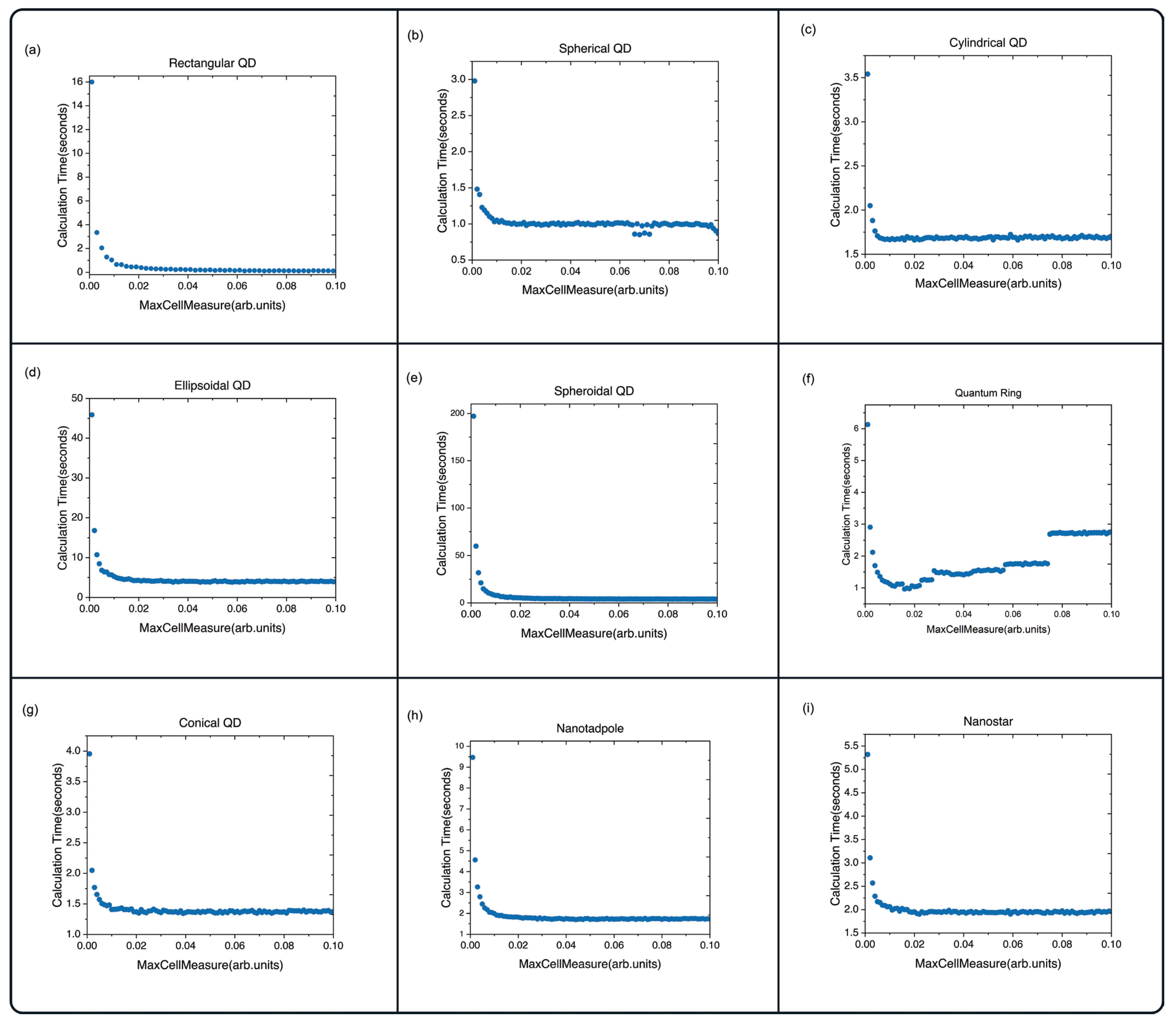
3.1. Acuracy and Computational Time

Before proceeding to the investigation of the energy spectrum, we should first showcase the limits of FEM’s accuracy. This can be conducted in several ways. The most direct method is by comparing the analytically obtainable energy values to the results obtained numerically. In general, we can assume that the numerical error increases for states with higher energy. The deviation from the exact analytical solution in the current article is defined as d = 1 E F E M / E A n a l y t i c ; its minimum value is 0 (exact solution). The deviations for the rectangular, spherical, and cylindrical QDs for the first twenty-six excited states are shown in Figure 3. As we can see, the solution with the least deviation is obtained for the rectangular QD (Figure 3a), and the solution with the most deviation and unpredictable behavior corresponds to the cylindrical QD. However, it is important to note that the deviation, even in the worst-case scenario, is less than 5%.
For the QDs with nontrivial geometry, the accuracy of FEM highly depends on how well the element mesh approximates the structure (region). Some geometrical parameters such as extreme angles (near 180° or near 0°) can cause large discretization errors. Decreasing the size of the elements will increase the accuracy but cost more computational time, so it is important to find an optimal value for this parameter. To that end, we calculated the ground-state energy E g r o u n d dependence on the MaxCellMeasure parameter. FEM generally overestimates the energy values. We can assume that the lower the ground-state energy, the higher the accuracy of the solution. Thus, in Figure 4, the dependence of the ground-state energy on the MaxCellMeasure parameter is presented for the rectangular (a), spherical (b), cylindrical (c), ellipsoidal (d), spheroidal (e), and conical (g) QDs as well as QR (f), nanotadpoles (h), and nanostars (i). The parameter was varied in the range of 0.001 0.1 ; we can see that universally, the lowest value for E g r o u n d is at the MaxCellMeasure 0.001 , which was to be expected. The most extreme decrease in energy is present for QRs and ellipsoidal QDs, meaning that their geometries are the hardest to approximate with tetrahedral mesh elements used in Mathematica. However, it is visible that for most cases, the energy decrease is in the order of 0.1   meV , which is negligible for most applications, so larger mesh elements of MaxCellMeasure 0.01   can be comfortably used. However, in the case of the ellipsoidal QD and the QR, we can see that the energy difference is in the order of 1 m e V , which cannot be neglected. The reverse side of the coin is the computation time, which increases with the decrease in the mesh element size. The time for obtaining the first ten eigenvectors and eigenvalues for the abovementioned QDs is presented in Figure 5. The results again solidify the fact that for spheroidal QDs, decreasing the size of the mesh elements is a poor choice because the increase in computation time is the highest for it; however, the accuracy decrease is negligible.
The results for the QRs showcase the relatively low time of 6 s for the MaxCellMeasure 0.001; this makes the decrease in the MaxCellMeasure worthwhile. Lastly, although the computation cost for the ellipsoidal QD is the second highest at 46 s, the accuracy increase cannot be neglected, and the lowest possible value should be taken for the best results. It is important to note that the discretization errors can be mitigated by the construction of custom meshes that use hexahedral elements, or maybe even hybrid meshes consisting of hexahedral and tetrahedral elements that take into account the symmetry of the QDs more accurately. However, we believe that this is beyond the scope of this paper.

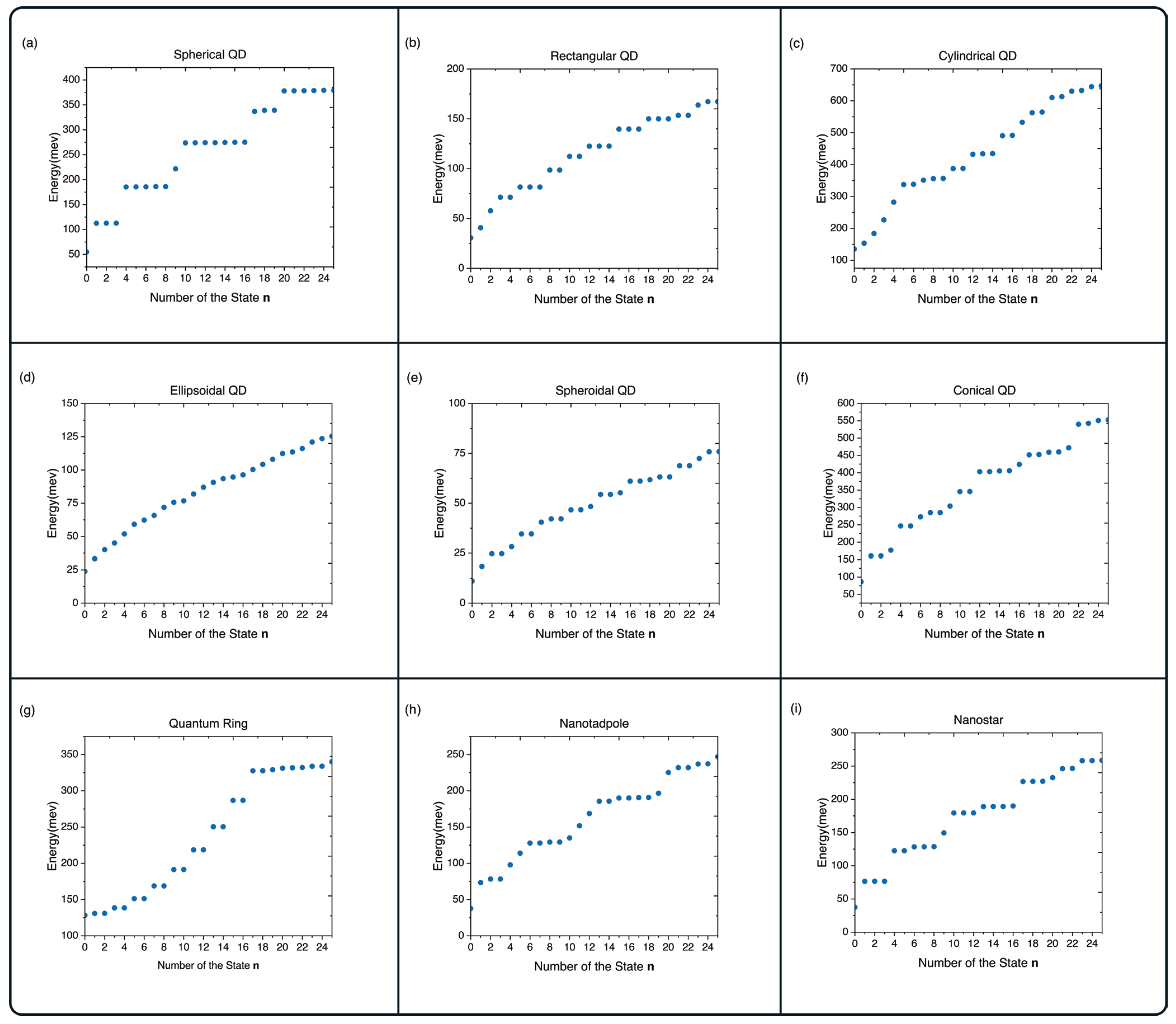
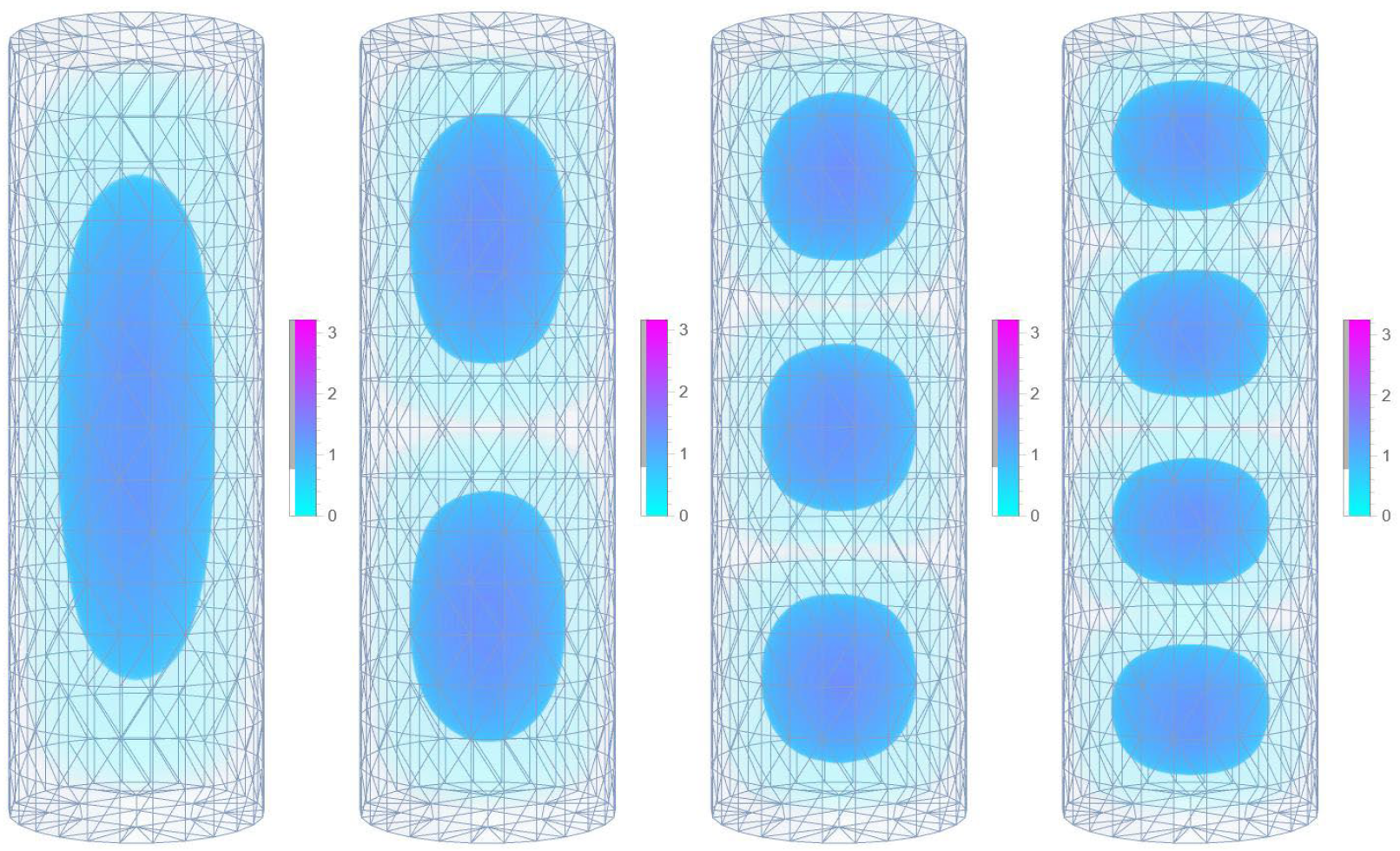
3.2. Electronic Energy and Wavefunctions of Semiconductor QDs

The energy of the particle localized in a QD strongly depends on the size quantization effects. This effect is what makes the spectrum of the QDs discrete. The size quantization effect depends on the material parameters of the structure, the size of the structure, and finally the shape of the structure. The size quantization not only shapes the energetic spectrum but also the wave function of the confined particle. As we know, the wave functions of the state differ in size, shape, and orientation. The size quantization affects all of these features, and the changes in the probability density cause changes in the difference between the energy levels, number of degenerate states, etc. That is why understanding the energetic spectrum of QD requires a parallel analysis of the probability density.
Let us start from the simplest case: an electron confined in the spherical QD. The energy spectrum is shown in Figure 6a and the probability densities for the first four states are shown in Figure 7. As we can see, the ground state has spherical symmetry and has no orbital nodes. The excited-state probability densities have one orbital node and are oriented in three different directions. Because of the spherical symmetry, each direction is equivalent to the other, and states that are defined by the same number of orbital nodes that only differ in orientation are energetically degenerate. The degeneracy of the energy spectrum is consistent with the well-known analytical solutions.
The situation changes in the case of a rectangular QD with geometrical parameters are similar to the ones taken in our calculation L x = 40   nm , L y = 20   nm , L z = 20   nm . As we can see here, the y- and z-directions have the same amount of size quantization. However, the size quantization is weak in the x-directions. The degeneracy remains for wave functions oriented towards the y- and z-directions, and this is reflected both by the probability densities (Figure 8) and the energy spectrum (Figure 6b). If the probability density is oriented in the x-direction, the resulting state has lower energy. This effect is tangible to the point that the wavefunction with two orbital nodes oriented in the x-direction has lower energy than wavefunctions with one orbital node oriented in the y- and z-directions.
This effect of the reordering of energy levels caused by the weaker size quantization in one direction is much more pronounced in the case of cylindrical QDs. The energy spectrum (Figure 6c) shows a nondegenerate behavior up to the sixth state, and this is displayed in the probability density (Figure 9), where for the first five states, the number of the nodes increases with each state, and the sixth and seventh states are the first states that are not oriented in the z-direction and have one orbital node. The subsequent behavior of the energetic spectrum can be explained similarly.
The first structure with the nontrivial geometry that we are going to present is the ellipsoidal QD with the following geometrical parameters: a x = 30   nm , b y = 10   nm , c z = 20   nm . All three half-axes have different values. This means that each direction has a different size quantization, which leads to the elimination of energetic degeneracy.
This is visible by the fact that the fourth state’s wave function does not have one node and is not oriented in the y-direction. Instead, the state with the one-node wavefunction oriented towards the y-axis corresponds to the seventh state (see Figure 10).
We know that an ellipsoid becomes a sphere if all of the half-axes are equal to each other, and becomes a spheroid when two of the half-axes are equal. As such, we can expect that an electron confined in a spheroidal QD will have a hybrid behavior between an ellipsoid and a sphere. The expected behavior is shown in Figure 11. The ground state has elliptic symmetry, and the first three excited states all have one node similar to the spherical case. However, the difference arises from the fact that the wavefunction of the first excited state is oriented in the z-direction and subsequently has weaker size quantization, causing the first excited state to lose its degeneracy. The energy spectrum continues this behavior to the higher states. It is important to note that for each case, the ratio of the unequal direction to the equal directions plays a crucial role, and the spectrum will reorder itself depending on the geometrical parameters.
This effect is caused by the directional non-equivalence and can be observed in any structure that has initial asymmetries. An example of such a structure is conical QDs (Figure 6f and Figure 12). The first two excited states have the same energies and wavefunctions, only differing in their orientation. The third excited state is oriented towards the z-direction, and has a higher energetic value because the electron is localized near the peak. Similar behavior can be observed in the energetic spectrum for the higher levels.
The reverse picture can be observed for a nanotadpole. Here, we have a structure that is comprised of two regions: a head region approximated with a sphere, and a tail region approximated with a cylinder merged to the head in the z-direction. This asymmetry in the z-direction leads to the lowering of the size quantization and a highly unusual shape for the wave function. However, the shape for the second and third excited states almost matches the spherical QD. This means that the electronic probability density only “seeps through” to the tail region in the case when the wave function is to some extent oriented in the z-direction (Figure 13). The energetic spectrum (Figure 6h) shows the effects of this “seep through” with the partial elimination of degenerate levels.
However, the directional non-equivalence is partially eliminated if you have a symmetrical structure such as a nanostar, which is symmetrical towards the three axes. At the first glance, you can see in Figure 14 that the wavefunctions are extremely similar to the spherical case. However, the additional freedom provided by the points leads to the transformation of the wave functions in all directions. For the ground state, the difference is slightly visible; however, for the excited state, the most noticeable contribution is the change in the orientation, as you can see that the first three excited states are no longer aligned strictly to the x-, y- and z-axes.
Let us close this subsection with the QRs. Here, the structure’s symmetry leads to the most unique ground-state probability density that we have discussed. It has a ring-like shape and is distributed uniformly in the structure, creating a “ring of probability density”. The excited states have more shapes and more possible orientations compared to the sphere. In the first twenty-five states, there are four states with wavefunctions that have one orbital node. However, only two of them degenerate in energy in the second and third excited states (Figure 15). The other two correspond to the twentieth and twenty-second excited states, the former’s probability densities are comprised of two probability density “rings” outgoing from the center (similar to the rings of Saturn), and the latter’s two probability density “rings” are stacked on each other. These shape and orientation changes contribute to the extreme energy differences between the first two and last two states with one-node wavefunctions. If we look at the energy spectrum (Figure 6g), we can see that the states are doubly degenerate or near degenerate until the sixteenth state.
These results showcase the way in which we can control the overlap between electronic and excitonic states and the energy spectrum, and by extension, most of the optoelectronic properties of QD.

3.3. Properties of Semiconductor Core/Shell QDs

In this subsection, we are going to investigate the localization probability for electrons and holes confined in a CdSe/CdS core–shell spherical QD with an impurity in the center.
This type of structure can be approximated by a potential of the form (4) that is presented in Figure 2. Generally, core/shell structures are grown with materials that have a bigger potential depth in the core V 0 C d S e , so for medium and large core sizes R c o r e , the particles are localized in the core. Let us first discuss the electron localization probability of an electron in Figure 16a. If the electron’s energy is noticeably lower than the difference between the confinement potentials of the two materials V e 0 C d S V e 0 C d S e 100 meV, the electron is mostly localized in the core. However, by making the core radius smaller, the size quantization in the core becomes stronger and the electron’s probability density “seeps through” to the shell region more and more as the ground-state energy rises. The electron localization probability density’s dependence on the core radius R c o r e is presented in Figure 16a with the segmented blue line; the ground state energy is presented in the same graph with the red solid line. You can see that around the point R c o r e = 4.74 nm, about 80 % of the electron probability density is localized in the core. As the size of the core decreases, electron probability “seeps through” more and more to the shell, until at R c o r e = 2.2 nm, only 20 % is in the core. It is important to note that the V e 0 C d S V e 0 C d S e depends on the growing methods, and for different values the probability density will behave differently. This is also visible for the hole. The potential difference for the hole V h 0 C d S V h 0 C d S e is twice as large V h 0 C d S V h 0 C d S e 200 meV. The hole’s localization probability in the core (Figure 16b) reaches about 85 % at the core size R c o r e = 1.4 nm. This is drastically different from the electron, which means that for core size values of around 2.2 nm, the overlap between the electron and hole wave functions decrease to the point that the structure can be considered to have a quasi-type-II band structure. These kinds of structures have a plethora of advantages, including the fact that the exciton lifetime increases drastically.
Quasi-type-II structures are actively investigated experimentally. For example, in [77], the authors investigated the temperature dependence of spectral properties such as the band gap, bandwidth, and fluorescence intensity of CdSe/CdS dot-in-rod nanocrystals. Quasi-type-II structures were synthesized with core sizes of R c o r e = 2.3 nm. The values for quasi-type-II structure core size obtained by our calculations are very close to the experimental values, which attests to the quality of our chosen model.
Overall, we can say that FEM can not only be used to model one-material QDs but also core/shell, core/shell/shell, or dot-in-bulk structures successfully, even allowing us to obtain structures with quasi-type-II band alignment.

4. Conclusions

Summarizing the results obtained in the scope of the current paper, we can say that FEM can be used to model QDs with various trivial and nontrivial geometries as well as multimaterial QDs. To recap Section 3.1, the deviation between FEM and the analytically obtainable energy values of the first twenty-six states was less than d 0.05 for a M a x C e l l M e a s u r e = 0.01 . The dependence of the ground-state energy E g r o u n d on the element size M a x C e l l M e a s u r e showed a significant correlation for QRs and ellipsoidal QDs (in the order of 1 m e V ). This shows that these structures are hard to approximate by Mathematica’s default discretization algorithm. This is also reflected by the fact that the computation cost for obtaining the first ten wavefunctions and energies for ellipsoidal QD at the M a x C e l l M e a s u r e = 0.001 is the second highest at 46 s. However, despite this relatively large timeframe, the impact on accuracy cannot be neglected. The situation is much more positive for the QR: the time for completing the calculation with the same parameters is about 6 s. In Section 3.2 of Results and Discussion, the electronic energy spectrum and probability densities were investigated for rectangular, spherical, cylindrical, ellipsoidal, spheroidal, conical QDs, QRs, nanotadpole QDs, and nanostars. The dependence of the energy spectrum and wavefunction orientation on the size quantization effect’s directional non-equivalence was discussed in detail. The effect of various asymmetries of structures was obtained and discussed. In the last subsection of Results and Discussion, we obtained the particle’s localization probability in the core of the CdSe/CdS structure for the electron and the hole. It was found that it is possible to obtain a structure with a quasi-type-II band alignment using the model chosen in our calculations, and the core size values correspond to the experimentally obtained quasi-type-II structures. Overall, we can say that FEM is a flexible tool for modeling QDs with various parameters, and the accuracy largely depends on the chosen potential models and the constructed mesh.

Author Contributions

Conceptualization, D.B.H. and P.A.M.; methodology, G.A.M. and D.B.H.; software, G.A.M.; investigation, G.A.M. and D.B.H.; writing—original draft preparation, G.A.M. and D.B.H.; writing—review and editing, P.A.M.; visualization, G.A.M.; supervision, D.B.H. and P.A.M. All authors have read and agreed to the published version of the manuscript.

Funding

The work was supported by the Science Committee of RA, in the frames of the research project № 21SCG-1C008.

Data Availability Statement

Not applicable.

Conflicts of Interest

The authors declare no conflict of interest. The funders had no role in the design of the study; in the collection, analyses, or interpretation of data; in the writing of the manuscript; or in the decision to publish the results.

References

  1. Yuan, J.; Hazarika, A.; Zhao, Q.; Ling, X.; Moot, T.; Ma, W.; Luther, J.M. Metal halide perovskites in quantum dot solar cells: Progress and prospects. Joule 2020, 4, 1160–1185. [Google Scholar] [CrossRef]
  2. Selopal, G.S.; Zhao, H.; Wang, Z.M.; Rosei, F. Core/shell quantum dots solar cells. Adv. Funct. Mater. 2020, 30, 1908762. [Google Scholar] [CrossRef]
  3. Ding, C.; Wang, D.; Liu, D.; Li, H.; Li, Y.; Hayase, S.; Sogabe, T.; Masuda, T.; Zhou, Y.; Yao, Y.; et al. Over 15% Efficiency PbS Quantum-Dot Solar Cells by Synergistic Effects of Three Interface Engineering: Reducing Nonradiative Recombination and Balancing Charge Carrier Extraction. Adv. Energy Mater. 2022, 12, 2201676. [Google Scholar] [CrossRef]
  4. Zhao, Q.; Han, R.; Marshall, A.R.; Wang, S.; Wieliczka, B.M.; Ni, J.; Zhang, J.; Yuan, J.; Luther, J.M.; Hazarika, A.; et al. Colloidal Quantum Dot Solar Cells: Progressive Deposition Techniques and Future Prospects on Large-Area Fabrication. Adv. Mater. 2022, 34, 2107888. [Google Scholar] [CrossRef] [PubMed]
  5. Li, M.; Chen, S.; Zhao, X.; Xiong, K.; Wang, B.; Shah, U.A.; Gao, L.; Lan, X.; Zhang, J.; Hsu, H.Y.; et al. Matching Charge Extraction Contact for Infrared PbS Colloidal Quantum Dot Solar Cells. Small 2022, 18, 2105495. [Google Scholar] [CrossRef]
  6. Ogundele, A.K.; Mola, G.T. Ternary atoms alloy quantum dot assisted hole transport in thin film polymer solar cells. J. Phys. Chem. Solids 2022, 171, 110999. [Google Scholar] [CrossRef]
  7. Prasath, A.; Athika, M.; Duraisamy, E.; Selva Sharma, A.; Sankar Devi, V.; Elumalai, P. Carbon quantum dot-anchored bismuth oxide composites as potential electrode for lithium-ion battery and supercapacitor applications. ACS Omega 2019, 4, 4943–4954. [Google Scholar] [CrossRef]
  8. Xu, Z.; Tang, X.; Liu, Y.; Zhang, Z.; Chen, W.; Liu, K.; Yuan, Z. CsPbBr3 quantum dot films with high luminescence efficiency and irradiation stability for radioluminescent nuclear battery application. ACS Appl. Mater. Interfaces 2019, 11, 14191–14199. [Google Scholar] [CrossRef]
  9. Sun, B.; Chen, Y.; Tao, L.; Zhao, H.; Zhou, G.; Xia, Y.; Wang, H.; Zhao, Y. Nanorod array of SnO2 quantum dot interspersed multiphase TiO2 heterojunctions with highly photocatalytic water splitting and self-rechargeable battery-like applications. ACS Appl. Mater. Interfaces 2018, 11, 2071–2081. [Google Scholar] [CrossRef]
  10. Liu, J.; Zhu, M.; Mu, K.; Han, T.; Pan, Z.; Gan, Y.; Zhang, H.; Si, T. Engineering a novel microcapsule of Cu 9 S 5 core and SnS 2 quantum dot/carbon nanotube shell as a Li-ion battery anode. Chem. Commun. 2021, 57, 13397–13400. [Google Scholar] [CrossRef]
  11. Babu, B.; Kim, J.; Yoo, K. Nanocomposite of SnO2 quantum dots and Au nanoparticles as a battery-like supercapacitor electrode material. Mater. Lett. 2022, 309, 131339. [Google Scholar] [CrossRef]
  12. Nie, Y.; Liang, Z.; Wang, P.; Ma, Q.; Su, X. MXene-derived quantum dot@ gold nanobones heterostructure-based electrochemiluminescence sensor for triple-negative breast cancer diagnosis. Anal. Chem. 2021, 93, 17086–17093. [Google Scholar] [CrossRef] [PubMed]
  13. Aznar-Gadea, E.; Rodriguez-Canto, P.J.; Sánchez, S.A.; Martínez-Pastor, J.P.; Abargues, R. Luminescent CdSe Quantum Dot Arrays for Rapid Sensing of Explosive Taggants. ACS Appl. Nano Mater. 2022, 5, 6717–6725. [Google Scholar] [CrossRef]
  14. Zhu, C.; Wang, Q.; Sun, G.; Zhao, S.; Wang, Y.; Li, T.; Hao, X.; Artemyev, M.; Tang, J. High-Luminescence Electrospun Polymeric Microfibers In Situ Embedded with CdSe Quantum Dots with Excellent Environmental Stability for Heat and Humidity Wearable Sensors. Nanomaterials 2022, 12, 2288. [Google Scholar] [CrossRef] [PubMed]
  15. de França, C.C.L.; Meneses, D.; Silva, A.C.A.; Dantas, N.O.; de Abreu, F.C.; Petroni, J.M.; Lucca, B.G. Development of novel paper-based electrochemical device modified with CdSe/CdS magic-sized quantum dots and application for the sensing of dopamine. Electrochim. Acta 2021, 367, 137486. [Google Scholar] [CrossRef]
  16. Jamalipour, P.; Choobkar, N.; Abrishamkar, M.; Pournamdari, E. Design of fluorescent method for sensing toxic diazinon in water samples using PbS quantum dots-based gelatin. J. Environ. Sci. Health Part B 2022, 57, 720–728. [Google Scholar] [CrossRef]
  17. Galstyan, V. “Quantum dots: Perspectives in next-generation chemical gas sensors”—A review. Anal. Chim. Acta 2021, 1152, 238192. [Google Scholar] [CrossRef]
  18. Xavier, J.; Yu, D.; Jones, C.; Zossimova, E.; Vollmer, F. Quantum nanophotonic and nanoplasmonic sensing: Towards quantum optical bioscience laboratories on chip. Nanophotonics 2021, 10, 1387–1435. [Google Scholar] [CrossRef]
  19. Mohageg, M.; Mazzarella, L.; Anastopoulos, C.; Gallicchio, J.; Hu, B.L.; Jennewein, T.; Johnson, S.; Lin, S.Y.; Ling, A.; Marquardt, C.; et al. The deep space quantum link: Prospective fundamental physics experiments using long-baseline quantum optics. EPJ Quantum Technol. 2022, 9, 25. [Google Scholar] [CrossRef]
  20. Uppu, R.; Midolo, L.; Zhou, X.; Carolan, J.; Lodahl, P. Quantum-dot-based deterministic photon–emitter interfaces for scalable photonic quantum technology. Nat. Nanotechnol. 2021, 16, 1308–1317. [Google Scholar] [CrossRef]
  21. Zeuner, K.D.; Jons, K.D.; Schweickert, L.; Reuterskiöld Hedlund, C.; Nuñez Lobato, C.; Lettner, T.; Wang, K.; Gyger, S.; Scholl, E.; Steinhauer, S.; et al. On-demand generation of entangled photon pairs in the telecom C-band with InAs quantum dots. ACS Photonics 2021, 8, 2337–2344. [Google Scholar] [CrossRef] [PubMed]
  22. Xiao, S.; Wu, S.; Xie, X.; Yang, J.; Wei, W.; Shi, S.; Song, F.; Sun, S.; Dang, J.; Yang, L.; et al. Position-dependent chiral coupling between single quantum dots and cross waveguides. Appl. Phys. Lett. 2021, 118, 091106. [Google Scholar] [CrossRef]
  23. Anderson, M.; Müller, T.; Skiba-Szymanska, J.; Krysa, A.B.; Huwer, J.; Stevenson, R.M.; Heffernan, J.; Ritchie, D.A.; Shields, A.J. Coherence in single photon emission from droplet epitaxy and Stranski–Krastanov quantum dots in the telecom C-band. Appl. Phys. Lett. 2021, 118, 014003. [Google Scholar] [CrossRef]
  24. Jin, T.; Li, X.; Liu, R.; Ou, W.; Zhu, Y.; Wang, X.; Liu, J.; Huo, Y.; Ou, X.; Zhang, J. Generation of Polarization-Entangled Photons from Self-Assembled Quantum Dots in a Hybrid Quantum Photonic Chip. Nano Lett. 2022, 22, 586–593. [Google Scholar] [CrossRef]
  25. Moody, G.; Sorger, V.J.; Blumenthal, D.J.; Juodawlkis, P.W.; Loh, W.; Sorace-Agaskar, C.; Jones, A.E.; Balram, K.C.; Matthews, J.C.; Laing, A.; et al. Roadmap on integrated quantum photonics. J. Phys. Photonics 2022, 4, 012501. [Google Scholar] [CrossRef]
  26. Scappucci, G.; Kloeffel, C.; Zwanenburg, F.A.; Loss, D.; Myronov, M.; Zhang, J.J.; De Franceschi, S.; Katsaros, G.; Veldhorst, M. The germanium quantum information route. Nat. Rev. Mater. 2021, 6, 926–943. [Google Scholar] [CrossRef]
  27. Mortemousque, P.A.; Chanrion, E.; Jadot, B.; Flentje, H.; Ludwig, A.; Wieck, A.D.; Urdampilleta, M.; Bäuerle, C.; Meunier, T. Coherent control of individual electron spins in a two-dimensional quantum dot array. Nat. Nanotechnol. 2021, 16, 296–301. [Google Scholar] [CrossRef]
  28. Basso Basset, F.; Salusti, F.; Schweickert, L.; Rota, M.B.; Tedeschi, D.; Covre da Silva, S.F.; Roccia, E.; Zwiller, V.; Jöns, K.D.; Rastelli, A.; et al. Quantum teleportation with imperfect quantum dots. npj Quantum Inf. 2021, 7, 7. [Google Scholar] [CrossRef]
  29. Mortemousque, P.A.; Jadot, B.; Chanrion, E.; Thiney, V.; Bäuerle, C.; Ludwig, A.; Wieck, A.D.; Urdampilleta, M.; Meunier, T. Enhanced Spin Coherence while Displacing Electron in a Two-Dimensional Array of Quantum Dots. PRX Quantum 2021, 2, 030331. [Google Scholar] [CrossRef]
  30. Liu, M.; Yazdani, N.; Yarema, M.; Jansen, M.; Wood, V.; Sargent, E.H. Colloidal quantum dot electronics. Nat. Electron. 2021, 4, 548–558. Available online: https://www.nature.com/articles/s41928-021-00632-7 (accessed on 4 December 2022). [CrossRef]
  31. Yang, X.F.; Chen, X.S.; Lu, W.; Fu, Y. Effects of shape and strain distribution of quantum dots on optical transition in the quantum dot infrared photodetectors. Nanoscale Res. Lett. 2008, 3, 534–539. [Google Scholar] [CrossRef] [PubMed] [Green Version]
  32. Vinasco, J.A.; Radu, A.; Kasapoglu, E.S.İ.N.; Restrepo, R.L.; Morales, A.L.; Feddi, E.; Mora-Ramos, M.E.; Duque, C.A. Effects of geometry on the electronic properties of semiconductor elliptical quantum rings. Sci. Rep. 2018, 8, 13299. [Google Scholar] [CrossRef] [PubMed] [Green Version]
  33. Zhou, Z.Y.; Zheng, C.X.; Tang, W.X.; Tersoff, J.; Jesson, D.E. Origin of quantum ring formation during droplet epitaxy. Phys. Rev. Lett. 2013, 111, 036102. [Google Scholar] [CrossRef] [PubMed]
  34. Abbarchi, M.; Mastrandrea, C.A.; Vinattieri, A.; Sanguinetti, S.; Mano, T.; Kuroda, T.; Koguchi, N.; Sakoda, K.; Gurioli, M. Photon antibunching in double quantum ring structures. Phys. Rev. B 2009, 79, 085308. [Google Scholar] [CrossRef]
  35. Ramalingam, G.; Magdalane, C.M.; Kumar, B.A.; Yuvakkumar, R.; Ravi, G.; Jothi, A.I.; Rotte, N.K.; Murugadoss, G.; Ananth, A. Enhanced visible light-driven photocatalytic performance of CdSe nanorods. Environ. Res. 2022, 203, 111855. [Google Scholar] [CrossRef] [PubMed]
  36. Ke, X.; Zhang, J.; Dai, K.; Fan, K.; Liang, C. Integrated S-scheme heterojunction of amine-functionalized 1D CdSe nanorods anchoring on ultrathin 2D SnNb2O6 nanosheets for robust solar-driven CO2 conversion. Sol. RRL 2021, 5, 2000805. [Google Scholar] [CrossRef]
  37. Utterback, J.K.; Ruzicka, J.L.; Hamby, H.; Eaves, J.D.; Dukovic, G. Temperature-dependent transient absorption spectroscopy elucidates trapped-hole dynamics in CdS and CdSe Nanorods. J. Phys. Chem. Lett. 2019, 10, 2782–2787. [Google Scholar] [CrossRef]
  38. Liu, H.; Hao, J.; Li, J.; Cheng, J.; Gao, Y.; Lin, X.; Wang, K.; He, T. Spectral and nonlinear optical properties of quasi-type II CdSe/CdS nanotadpoles. J. Phys. Chem. C 2020, 124, 27840–27847. [Google Scholar] [CrossRef]
  39. Ma, Y.; Lan, K.; Xu, B.; Xu, L.; Duan, L.; Liu, M.; Chen, L.; Zhao, T.; Zhang, J.Y.; Lv, Z.; et al. Streamlined mesoporous silica nanoparticles with tunable curvature from interfacial dynamic-migration strategy for nanomotors. Nano Lett. 2021, 21, 6071–6079. [Google Scholar] [CrossRef]
  40. Hao, J.; Li, Y.; Miao, J.; Liu, R.; Li, J.; Liu, H.; Wang, Q.; Liu, H.; Delville, M.H.; He, T.; et al. Ligand-induced chirality in asymmetric CdSe/CdS nanostructures: A close look at chiral tadpoles. ACS Nano 2020, 14, 10346–10358. [Google Scholar] [CrossRef]
  41. Di Mari, G.M.; Mineo, G.; Franzò, G.; Mirabella, S.; Bruno, E.; Strano, V. Low-Cost, High-Yield ZnO Nanostars Synthesis for Pseudocapacitor Applications. Nanomaterials 2022, 12, 2588. [Google Scholar] [CrossRef] [PubMed]
  42. Veerakumar, P.; Sangili, A.; Saranya, K.; Pandikumar, A.; Lin, K.C. Palladium and silver nanoparticles embedded on zinc oxide nanostars for photocatalytic degradation of pesticides and herbicides. Chem. Eng. J. 2021, 410, 128434. [Google Scholar] [CrossRef]
  43. Manavalan, S.; Veerakumar, P.; Chen, S.M.; Lin, K.C. Three-dimensional zinc oxide nanostars anchored on graphene oxide for voltammetric determination of methyl parathion. Microchim. Acta 2020, 187, 17. [Google Scholar] [CrossRef]
  44. Abu-Hariri, A.; Budniak, A.K.; Horani, F.; Lifshitz, E. Star-shaped colloidal PbS nanocrystals: Structural evolution and growth mechanism. RSC Adv. 2021, 11, 30560–30568. [Google Scholar] [CrossRef] [PubMed]
  45. Wang, Y.; Ke, J.; Guo, X.; Gou, K.; Sang, Z.; Wang, Y.; Bian, Y.; Li, S.; Li, H. Chiral mesoporous silica nano-screws as an efficient biomimetic oral drug delivery platform through multiple topological mechanisms. Acta Pharm. Sin. B 2022, 12, 1432–1446. [Google Scholar] [CrossRef] [PubMed]
  46. Mishra, Y.K.; Adelung, R. ZnO tetrapod materials for functional applications. Mater. Today 2018, 21, 631–651. [Google Scholar] [CrossRef]
  47. Myndrul, V.; Iatsunskyi, I.; Babayevska, N.; Jarek, M.; Jesionowski, T. Effect of Electrode Modification with Chitosan and Nafion® on the Efficiency of Real-Time Enzyme Glucose Biosensors Based on ZnO Tetrapods. Materials 2022, 15, 4672. [Google Scholar] [CrossRef]
  48. Dixit, T.; Palani, I.A.; Singh, V. Investigation on the influence of dichromate ion on the ZnO nano-dumbbells and ZnCr2O4 nano-walls. J. Mater. Sci. Mater. Electron. 2015, 26, 821–829. [Google Scholar] [CrossRef]
  49. Eshet, H.; Grünwald, M.; Rabani, E. The electronic structure of CdSe/CdS core/shell seeded nanorods: Type-I or quasi-type-II? Nano Lett. 2013, 13, 5880–5885. [Google Scholar] [CrossRef] [Green Version]
  50. Baghdasaryan, D.A.; Hayrapetyan, D.B.; Kazaryan, E.M. Optical properties of narrow band prolate ellipsoidal quantum layers ensemble. J. Nanophotonics 2016, 10, 033508. [Google Scholar] [CrossRef]
  51. Hayrapetyan, D.B.; Bleyan, Y.Y.; Baghdasaryan, D.A.; Sarkisyan, H.A.; Baskoutas, S.; Kazaryan, E.M. Biexciton, negative and positive trions in strongly oblate ellipsoidal quantum dot. Phys. E Low-Dimens. Syst. Nanostruct. 2019, 105, 47–55. [Google Scholar] [CrossRef]
  52. Hayrapetyan, D.B.; Chalyan, A.V.; Kazaryan, E.M.; Sarkisyan, H.A. Direct interband light absorption in conical quantum dot. J. Nanomater. 2015, 16, 406. [Google Scholar] [CrossRef] [Green Version]
  53. Hayrapetyan, D.B.; Kazaryan, E.M.; Sarkisyan, H.A. On the possibility of implementation of Kohn’s theorem in the case of ellipsoidal quantum dots. J. Contemp. Phys. (Armen. Acad. Sci.) 2013, 48, 32–36. [Google Scholar] [CrossRef]
  54. Hayrapetyan, D.B.; Kazaryan, E.M.; Sarkisyan, H.A. Implementation of Kohn’s theorem for the ellipsoidal quantum dot in the presence of external magnetic field. Phys. E Low-Dimens. Syst. Nanostruct. 2016, 75, 353–357. [Google Scholar] [CrossRef]
  55. Garoufalis, C.S.; Zeng, Z.; Bester, G.; Hayrapetyan, D.B.; Baskoutas, S. Optical properties of zig-zag and armchair ZnO colloidal nanoribbons. Chem. Phys. Lett. 2019, 732, 136659. [Google Scholar] [CrossRef]
  56. Postica, V.; Gröttrup, J.; Adelung, R.; Lupan, O.; Mishra, A.K.; de Leeuw, N.H.; Mishra, Y.K. Multifunctional materials: A case study of the effects of metal doping on ZnO tetrapods with bismuth and tin oxides. Adv. Funct. Mater. 2017, 27, 1604676. [Google Scholar] [CrossRef]
  57. Malik, P.; Thareja, R.; Singh, J.; Kakkar, R. II-VI core/shell quantum dots and doping with transition metal ions as a means of tuning the magnetoelectronic properties of CdS/ZnS core/shell QDs: A DFT study. J. Mol. Graph. Model. 2022, 111, 108099. [Google Scholar] [CrossRef]
  58. David Müzel, S.; Bonhin, E.P.; Guimarães, N.M.; Guidi, E.S. Application of the finite element method in the analysis of composite materials: A review. Polymers 2020, 12, 818. [Google Scholar] [CrossRef] [Green Version]
  59. Dandekar, C.R.; Shin, Y.C. Modeling of machining of composite materials: A review. Int. J. Mach. Tools Manuf. 2012, 57, 102–121. [Google Scholar] [CrossRef]
  60. Lasri, L.; Nouari, M.; El Mansori, M. Modelling of chip separation in machining unidirectional FRP composites by stiffness degradation concept. Compos. Sci. Technol. 2009, 69, 684–692. [Google Scholar] [CrossRef]
  61. Zhao, L.G.; Warrior, N.A.; Long, A.C. Finite element modelling of damage progression in non-crimp fabric reinforced composites. Compos. Sci. Technol. 2006, 66, 36–50. [Google Scholar] [CrossRef]
  62. Mantashian, G.A.; Zaqaryan, N.A.; Mantashyan, P.A.; Sarkisyan, H.A.; Baskoutas, S.; Hayrapetyan, D.B. Linear and Nonlinear Optical Absorption of CdSe/CdS Core/Shell Quantum Dots in the Presence of Donor Impurity. Atoms 2021, 9, 75. [Google Scholar] [CrossRef]
  63. Hayrapetyan, D.B.; Amirkhanyan, S.M.; Kazaryan, E.M.; Sarkisyan, H.A. Effect of hydrostatic pressure on diamagnetic susceptibility of hydrogenic donor impurity in core/shell/shell spherical quantum dot with Kratzer confining potential. Phys. E Low-Dimens. Syst. Nanostruct. 2016, 84, 367–371. [Google Scholar] [CrossRef]
  64. Mantashian, G.A.; Mantashyan, P.A.; Sarkisyan, H.A.; Kazaryan, E.M.; Bester, G.; Baskoutas, S.; Hayrapetyan, D.B. Exciton-Related Raman Scattering, Interband Absorption and Photoluminescence in Colloidal CdSe/CdS Core/Shell Quantum Dots Ensemble. Nanomaterials 2021, 11, 1274. [Google Scholar] [CrossRef] [PubMed]
  65. Cristea, M. Simultaneous effects of electric field, shallow donor impurity and geometric shape on the electronic states in ellipsoidal ZnS/CdSe core-shell quantum dots. Phys. E Low-Dimens. Syst. Nanostruct. 2018, 103, 300–306. [Google Scholar] [CrossRef]
  66. Choubani, M.; Maaref, H.; Saidi, F. Nonlinear optical properties of lens-shaped core/shell quantum dots coupled with a wetting layer: Effects of transverse electric field, pressure, and temperature. J. Phys. Chem. Solids 2020, 138, 109226. [Google Scholar] [CrossRef]
  67. Bhagyaraj, S.; Perumbilavil, S.; Udayabashkar, R.; Mangalaraja, R.V.; Thomas, S.; Kalarikkal, N.; Oluwafemi, O.S. Tuning of nonlinear absorption in highly luminescent CdSe based quantum dots with core–shell and core/multi-shell architectures. Phys. Chem. Chem. Phys. 2019, 21, 11424–11434. [Google Scholar] [CrossRef]
  68. Osorio, J.A.; Caicedo-Paredes, D.; Vinasco, J.A.; Morales, A.L.; Radu, A.; Restrepo, R.L.; Martínez-Orozco, J.C.; Tiutiunnyk, A.; Laroze, D.; Hieu, N.N.; et al. Pyramidal core-shell quantum dot under applied electric and magnetic fields. Sci. Rep. 2020, 10, 8961. [Google Scholar] [CrossRef]
  69. Mora-Ramos, M.E.; El Aouami, A.; Feddi, E.; Radu, A.; Restrepo, R.L.; Vinasco, J.A.; Morales, A.L.; Duque, C.A. Donor impurity energy and optical absorption in spherical sector quantum dots. Heliyon 2020, 6, e03194. [Google Scholar] [CrossRef] [Green Version]
  70. Mantashian, G.A.; Hayrapetyan, D.B. Impurity effects on binding energy, diamagnetic susceptibility, and photoionization cross-section of chalcopyrite AgInSe2 Nanotadpole. J. Phys. Condens. Matter 2022, 34, 245302. [Google Scholar] [CrossRef]
  71. Pulgar-Velásquez, L.; Sierra-Ortega, J.; Vinasco, J.A.; Laroze, D.; Radu, A.; Kasapoglu, E.; Restrepo, R.L.; Gil-Corrales, J.A.; Morales, A.L.; Duque, C.A. Shallow donor impurity states with excitonic contribution in GaAs/AlGaAs and CdTe/CdSe truncated conical quantum dots under applied magnetic field. Nanomaterials 2021, 11, 2832. [Google Scholar] [CrossRef]
  72. Chnafi, M.; Belamkadem, L.; Mommadi, O.; Boussetta, R.; El Hadi, M.; El Moussaouy, A.; Falyouni, F.; Vinasco, J.A.; Laroze, D.; Mora-Rey, F.; et al. Hydrostatic pressure and temperature effects on spectrum of an off-center single dopant in a conical quantum dot with spherical edge. Superlattices Microstruct. 2021, 159, 107052. [Google Scholar] [CrossRef]
  73. Dash, R.; Jena, S. Finite element analysis of the effect of wetting layer on the electronic eigenstates of InP/InGaP pyramidal quantum dots solar cell. Mater. Today Proc. 2021, 39, 2015–2021. [Google Scholar] [CrossRef]
  74. El Aouami, A.; Bikerouin, M.; Feddi, K.; Aghoutane, N.; El-Yadri, M.; Feddi, E.; Dujardin, F.; Radu, A.; Restrepo, R.L.; Vinasco, J.A.; et al. Linear and nonlinear optical properties of a single dopant in GaN conical quantum dot with spherical cap. Philos. Mag. 2020, 100, 2503–2523. [Google Scholar] [CrossRef]
  75. Cui, J.; Panfil, Y.E.; Koley, S.; Shamalia, D.; Waiskopf, N.; Remennik, S.; Popov, I.; Oded, M.; Banin, U. Colloidal quantum dot molecules manifesting quantum coupling at room temperature. Nat. Commun. 2019, 10, 5401. [Google Scholar] [CrossRef] [Green Version]
  76. Costa, L.S.D.; Prudente, F.V.; Acioli, P.H.; Neto, J.S.; Vianna, J.D.M. A study of confined quantum systems using the Woods-Saxon potential. J. Phys. B At. Mol. Opt. Phys. 1999, 32, 2461. [Google Scholar] [CrossRef] [Green Version]
  77. Wen, X.; Sitt, A.; Yu, P.; Toh, Y.R.; Tang, J. Temperature dependent spectral properties of type-I and quasi type-II CdSe/CdS dot-in-rod nanocrystals. Phys. Chem. Chem. Phys. 2012, 14, 3505–3512. [Google Scholar] [CrossRef]
Figure 1. The mesh regions used for the calculations: (a) mesh for a rectangular QD, (b) mesh for a spherical QD, (c) mesh for a conical QD, (d) mesh for a cylindrical QD, (e) mesh for an ellipsoid QD, (f) mesh for an ellipsoid of revolution (spheroid), (g) mesh for a nanotadpole, (i) mesh for a nanostar, (j) mesh for the quantum ring.
Computation 11 00005 g001
Figure 2. Piecewise Woods–Saxon potential plotted for the following parameters: R c o r e = 1   nm , R s h e l l = 1.3   nm , a c o r e = 0.03 .
Computation 11 00005 g002
Figure 3. The deviation of the analytically obtained electron energy value from the numerical values for the first 26 states in (a) rectangular, (b) spherical, and (c) cylindrical QDs. The comparison was carried out for the M a x C e l l M e a s u r e = 0.01 .
Computation 11 00005 g003
Figure 4. The dependence of the electron energy on the MaxCellMeasure parameter for (a) rectangular QDs, (b) spherical QDs, (c) cylindrical QDs, (d) ellipsoidal QDs, (e) spheroidal QDs, (f) QRs, (g) conical QDs, (h) nanotadpole QDs, (i) nanostars.
Computation 11 00005 g004
Figure 5. The dependence of computation time of the first 10 states on the MaxCellMeasure parameter for (a) rectangular QDs, (b) spherical QDs, (c) cylindrical QDs, (d) ellipsoidal QDs, (e) spheroidal QDs, (f) QRs, (g) conical QDs, (h) nanotadpole QDs, (i) nanostars.
Computation 11 00005 g005
Figure 6. The values of energy for the electron’s ground state and the first twenty-five excited states for (a) rectangular QDs, (b) spherical QDs, (c) cylindrical QDs, (d) ellipsoidal QDs, (e) spheroidal QDs, (f) QRs, (g) conical QDs, (h) nanotadpole QDs, (i) nanostars.
Computation 11 00005 g006
Figure 7. The probability density of the ground state and first three excited states of an electron confined in a spherical GaAs QD. The mesh domain used for the calculation is overlaid on the probability density.
Computation 11 00005 g007
Figure 8. The probability density of the ground state and first three excited states of an electron confined in a rectangular GaAs QD. The mesh domain used for the calculation is overlaid on the probability density.
Computation 11 00005 g008
Figure 9. The probability density of the ground state and first three excited states of an electron confined in a cylindrical GaAs QD. The mesh domain used for the calculation is overlaid on the probability density.
Computation 11 00005 g009
Figure 10. The probability density of the ground state and first three excited states of an electron confined in an ellipsoidal GaAs QD. The mesh domain used for the calculation is overlaid on the probability density.
Computation 11 00005 g010
Figure 11. The probability density of the ground state and first three excited states of an electron confined in a spheroidal GaAs QD. The mesh domain used for the calculation is overlaid on the probability density.
Computation 11 00005 g011
Figure 12. The probability density of the ground state and first three excited states of an electron confined in a conical GaAs QD. The mesh domain used for the calculation is overlaid on the probability density.
Computation 11 00005 g012
Figure 13. The probability density of the ground state and first three excited states of an electron confined in a conical GaAs nanotadpole. The mesh domain used for the calculation is overlaid on the probability density.
Computation 11 00005 g013
Figure 14. The probability density of the ground state and first three excited states of an electron confined in a GaAs nanostar. The mesh domain used for the calculation is overlaid on the probability density.
Computation 11 00005 g014
Figure 15. The probability density of the ground state and first three excited states of an electron confined in a GaAs QR. The mesh domain used for the calculation is overlaid on the probability density.
Computation 11 00005 g015
Figure 16. The segmented blue line is the probability density of the particle’s ground state localized in the core region, the solid red line is the ground state energy of the particle depending on the inner core size for an electron (a) and a hole (b). In (a), you can see three regions: the region that has a red pattern represents the core radii where the localization probability of the hole in the core is less than 50 % . The second region, represented by the red and blue pattern, shows the core radii where the hole’s localization probability in the core is larger than 50 % but the electron’s localization probability is lower than 50 % . The third region does not have a pattern, and shows the core radii where both the hole’s and the electron’s localization probability in the core are larger than 50 % .
Computation 11 00005 g016
Table 1. Geometrical parameters of structures in the calculations.
The StructureValues of Geometrical Parameters (nm)
Rectangular QD L x = 40 , L y = 20 , L z = 20
Spherical QD R = 10
Cylindrical QD R = 5 , H = 30
Ellipsoidal QD a x = 30 , b y = 10 , c z = 20 ,
Spheroidal QD a = 30 , b = 20 , c = 20
QR R i n n e r = 10 , R o u t e r = 20
Conical QD R = 12 , H = 20
Nanotadpole R h e a d = 12 , R t a i l = 6 , H t a i l = 20
Nanostar R s p h e r e = 10 , R c o n e = 10 , H c o n e = 7.5
Table 2. Geometrical parameters of structures in the calculations.
Part NameModel
CPUAMD Ryzen Thresadripper 3990X
RAMKingston 4 × 32 GB 3600 MHz
GPUDouble NVIDIA GeForce RTX 3090
Disclaimer/Publisher’s Note: The statements, opinions and data contained in all publications are solely those of the individual author(s) and contributor(s) and not of MDPI and/or the editor(s). MDPI and/or the editor(s) disclaim responsibility for any injury to people or property resulting from any ideas, methods, instructions or products referred to in the content.

