Procedure Used to Estimate the Power Production of a Photovoltaic Module Operating under Partial Shading Conditions

Abstract

This paper presents a methodology used to estimate the energy generated during one year by a photovoltaic module (PVM) operating under partial shading conditions. The methodology starts by calculating the solar paths and contours of nearby objects that produce shadows. Then, a method was proposed to estimate the shading factors of each submodule. Afterwards, the solar resource data and the calculated shading factors were used to feed a detailed PVM model to calculate the power–voltage curves for each hour, which were used to obtain a power profile and estimate the energy generated by the PVM in one year. The procedure was validated through simulation and experimental results. The simulation results consider a case study available in the literature, which was simulated to evaluate the effect on the PVM energy estimation considering and disregarding the partial shading conditions. The experimental results illustrate the capacity of the proposed methodology to predict the shaded and unshaded submodules and the module power–voltage curve. The results show that the proposed method avoids the energy overestimation introduced by classical estimation methods, which affects the sizing of a photovoltaic generator.

1. Introduction

In order to achieve an expansion of the photovoltaic (PV) market, it is necessary to improve the knowledge of the energy production of those systems. Depending on the location, it is necessary to precisely estimate the economic profitability, which requires taking into account the effects of shades on the energy generation [1]. Those partial shading conditions can occur due to the proximity of the PV module (PVM) to buildings, trees, and street furniture, among others. In addition, the shadows cast on a PVM due to nearby objects vary throughout the day and year due to the translation and rotation of the Earth around the sun.

There are different procedures proposed in the literature used to estimate the energy production of the PVM considering the effect of partial shading in a simplified way, without using detailed generator models, to calculate the effect of partial shading on the power production [2,3,4,5]. Other procedures use models designed to estimate both local and global maximum power points, but those methods are difficult to use directly when accounting for the power generation over relatively long periods (for example, one year) [6,7,8].

Several papers present procedures used to estimate the maximum power point when a PVM is operating under partial shading conditions [9,10,11,12,13,14,15]. However, those procedures do not allow for an estimation of the power generation profile for a photovoltaic array considering the variation in the shadow hour by hour during a year, because those methods are focused on performing analyses in a particular instant of time. In addition, the implementation of the methods requires a large computing capacity due to the models’ complexity.

In general, the procedures developed to estimate the hourly power profile disregard the losses due to partial shading over the modules [16,17,18], but, in some other cases, those losses are included within a global efficiency factor [2,3,5]. However, those procedures do not allow for estimating the losses due to the variation in the incident shading in the PV array due to changes in the sun’s trajectory throughout the year, thus reducing the estimation precision.

Other works are focused on providing a shading factor; for example, in [19], a vertical and horizontal shading factor is estimated for photovoltaic arrays. Similarly, in [4], a shading factor is calculated as an implicit value in an instantaneous efficiency factor of the PV system. On the other hand, the authors of [20,21] present a design methodology that considers the relative trajectories between the sun and the Earth, also including the position of surrounding objects that generate partial shading over the PVM. Nevertheless, all of those methodologies have a low accuracy since they use approximations, and do not take the PVM model into consideration when it is operating under partial shading conditions.

The effects of partial shading on the power losses are not intuitive, and such losses must be quantified using simulation software every hour throughout the year [22]. Software tools, such as PVSYST [23], allow us to find a power profile hour by hour considering the variation in shadows along the year with a reasonable computation time. However, to estimate the power–voltage (P-V) curve for each instant of time, considering the shadows effect, PVSYST uses an extrapolation of the current–voltage (I-V) curves of each module using fixed shading factors for each module in the generator, which is not accurate enough. Moreover, the methods used to obtain both the I-V curves and the shading factors are not clear [22].

In [24], a summary of shading analyzers is reported that describes some devices developed to analyze the shading effects produced by nearby objects, such as Amethyst [25], Hat [26], SUNDI [27], and Sun eye [28]. However, these devices do not provide shading information that can be used in PVM models, and they do not report the algorithm used to consider the partial shading effect in the energy estimation.

Other analyzers, such as Asset and PVWatts [29], consider the real position of the sun as irrelevant for the analysis, and they do not allow for an accurate detection of the shading factor change over time. Moreover, the Horizon catchers [30] provide a fast analysis with high precision, but they are expensive devices and do not use the PVM model to estimate the power generation.

There are two important points extracted from the previous discussion: on the one hand, despite the shading analyzers allowing for the evaluation of the effects of shading during a year, most of those devices contain complex hardware and software that are closed for the users. On the other hand, those analyzers use extrapolations or approximations to obtain the I-V curves, or a non-explained model, which makes it difficult to analyze and evaluate the accuracy of those devices.

This paper proposes a methodology used to estimate the energy production of a PVM operating under partial shading conditions. The methodology begins by calculating the solar paths for the geographic location of the PVM. Then, it constructs the shading profile produced by the surrounding objects with respect to a corner of the PVM, which is extrapolated to the other corners of the submodules into the PVM. From such information, the methodology estimates the shading factors of each submodule in the PVM for each hour of the year, which are used by a PVM model to calculate the P-V curve to identify both local and global maximum power points. Finally, an hourly power profile is generated from the global maximum power points to calculate the energy generated by the PVM. The proposed methodology is validated using detailed simulations to evaluate the effect of considering or neglecting the partial shading conditions on the energy production of a PVM. Finally, the experimental results show the capacity of the proposed methodology to predict the shaded and unshaded submodules in a PVM, as well as to reproduce the P-V curves to determine the local and global maximum power points.

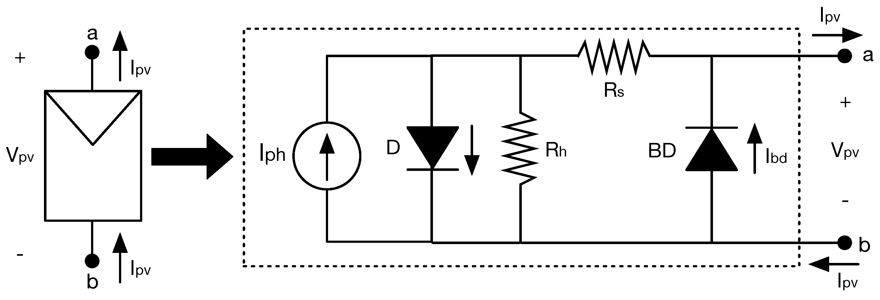
2. Photovoltaic Module (PVM) Model

Commercial PV modules are formed by series-connected submodules, each one of them protected by a bypass diode [31]. This paper used the model proposed in [32] to calculate the current–voltage (I-V) and power–voltage (P-V) curves of a PVM operating under partial shading conditions. Such a model uses the single-diode equivalent circuit to represent each submodule of the PVM, which provides a trade-off between complexity and accuracy.

The single-diode model for a PV submodule, depicted in Figure 1, is formed by a current source ($I_{ph}$) that represents the photovoltaic effect, a diode D (with $I_d$ current) that represents the nonlinear behavior of the P-N junctions, two resistors ($R_s$ and $R_h$) representing the main losses, and a bypass diode (BD) protecting the submodule’s cells [31]. In Figure 1, the dotted block describes the structure of the single-diode model, including the bypass diode.

The mathematical expression for PV current $I_{pv}$ in the single-diode model is given in Equations (1)–(3), where $V_{pv}$ is the voltage at the submodule terminals, $N_s$ is the number of the series-connected cells forming the submodule, $I_s$ is the inverse-saturation current of the submodule, and $V_t=n·k·T_{cells}/q$ is the thermal voltage of the submodule, where n is the ideality factor, k is the Boltzmann constant, q is the electron charge, and $T_{cells}$ is the temperature of the submodules’ cells. Moreover, $I_s,BD$ is the inverse-saturation current of the bypass diode, and $V_{t,BD}=n_{BD}·k·T_{BD}/q$ is the thermal voltage of the bypass diode, where $n_{BD}$ is the ideality factor of the diode and $T_{BD}$ is the temperature of the bypass diode. Since the bypass diode is located very close to the submodule’ cells (in the junction box at the back of the submodule), such a temperature is considered as equal to the temperature of the submodules’ cells.

$$\begin{array}{c}\hfill I_{pv}=-\frac{N_s·V_t·W\left({\theta }_1\right)}{R_s}+I_{s,BD}\left(e^{-V_{pv}/V_{t,BD}}-1\right)+\frac{R_h·\left(I_{ph}+I_s\right)-V_{pv}}{R_h+R_s}\end{array}$$

(1)

$$\begin{array}{c}\hfill {\theta }_1=\left(\frac{R_h·R_s}{R_h+R_s}\right)·\frac{I_s}{N_s·V_t}·e^{{\theta }_2}\end{array}$$

(2)

$$\begin{array}{c}\hfill {\theta }_2=\frac{\left(R_h+R_s\right)·\left(I_{ph}+I_s\right)·R_h·V_{pv}}{N_s·V_t·\left(R_h+R_s\right)}\end{array}$$

(3)

Therefore, the two main inputs of the single-diode model are the solar irradiance (G) and ambient temperature ($T_a$), and the two main outputs are the submodule current ($I_{pv}$) and voltage ($V_{pv}$), which can be used to calculate the submodules power as $P_{pv}=V_{pv}·I_{pv}$. The temperature of the submodules’ cells can be estimated from $T_a$ and G, as shown in (4), where $T_{NOCT}$ is the nominal operating cell temperature. Such a temperature is given in Kelvin degrees ([K]); hence, $T_a$ and $T_{NOCT}$ must also be expressed in [K].

$$T_{cells}=T_a+G\left(\frac{T_{NOCT}-(20+273.15)}{800}\right)$$

(4)

The parameter $I_{ph}$ can be calculated by using (5), where $F_S$ is a shading factor, $G_{STC}$ and $I_{ph,STC}$ are the irradiance and $I_{ph}$ in standard test conditions (STC), respectively, and ${\alpha }_{Isc}$ is the thermal coefficient of the PVM short-circuit current (provided in the manufacturer’ datasheet). The shading factor is a dimensionless value between 0 and 1 that represents the irradiance reduction on a submodule produced by a shadow.

$$I_{ph}=F_S\left(\frac{G}{G_{STC}}\right)\left(I_{ph,STC}+{\alpha }_{Isc}\left(T_{\mathit{cells}}-T_{STC}\right)\right)$$

(5)

The model proposed in [32] requires a shading factor for each submodule to calculate the P-V curve for a given operating condition; therefore, the shading factors are organized in a vector ($F_{sv}$), where the number of elements corresponds to the number of submodules in the PVM. For example, for a PVM with three submodules without shadow, the vector would be $F_{sv}=\left[F_{S1}{F}_{S2}{F}_{S3}\right]=\left[111\right]$, where $F_{S1}$, $F_{S2}$, and $F_{S3}$ are the shading factors of submodules 1 (S1), 2 (S2), and 3 (S3), respectively.

3. Proposed Methodology to Estimate the Energy of a PVM

The objective of this methodology is to estimate a power profile of one year (hour by hour) for a PV panel operating under partial shading conditions produced by surrounding objects. The proposed methodology is composed by five elements: (i) calculation of solar paths, (ii) calculation of the shading contour for a module point, (iii) extrapolation of shading contours to the key points of the PVM, (iv) estimation of the shading factors, and (v) power profile calculation to estimate the generated energy. The description of those elements is given in the following subsections.

3.1. Calculation of Solar Paths

The position of the sun in the sky can be represented by two angles: azimuth ($\gamma$) and elevation ($\alpha$). The azimuth is the angle between the north and the projection of the direction of the sun in a horizontal plane at a tangent to the surface of the earth, whereas the elevation is the angle between the direction of the sun (center of the solar disk) and the horizontal plane [20]. These two angles depend on the declination angle of the earth ($\delta$), the latitude of the point of interest ($\varphi$), the solar hour angle (w), and solar time (TLT), as shown in Equations (6) and (7) [21].

$$\begin{array}{c}\hfill \alpha ={sin}^{-1}(sin\left(\delta \right)sin\left(\varphi \right)+cos\left(\delta \right)cos\left(\varphi \right)cos\left(w\right))\end{array}$$

(6)

$$\begin{array}{c}\hfill \gamma =\left\{\begin{array}{c}{180}^{\circ }-{cos}^{-1}\left(\frac{sin\left(\alpha \right)sin\left(\varphi \right)-sin\left(\delta \right)}{cos\left(\alpha \right)cos\left(\varphi \right)}\right),\mathrm{if}TLT\le 12\mathrm{h}\hfill \\ {180}^{\circ }+{cos}^{-1}\left(\frac{sin\left(\alpha \right)sin\left(\varphi \right)-sin\left(\delta \right)}{cos\left(\alpha \right)cos\left(\varphi \right)}\right),\mathrm{if}TLT>12\mathrm{h}\hfill \end{array}\right.\end{array}$$

(7)

In turn, $\delta$, $\varphi$, w, and $TLT$ change throughout the year and depend on the geographical location of the point of interest, the date, and the time at which it is required to calculate the position of the sun [21]. The angle $\delta$ can be calculated using (8), where n is an integer representing the day of the year $(n\in [1,\cdots ,365\left]\right)$. The solar time ($TLT$) is calculated using (9), where $CET$ is the Central European summer time in [h], $L_c$ is the longitudinal correction in [min], and $E_t$ is the solar time equation in [min]. In (9), $E_t$ is calculated from (10), where $B=360(n-1)/365$, and $L_c$ is calculated using (11), where 4 is given in [min/°], $L_{zone}$ is the standard time meridian in [°], and $L_{local}$ is the local time meridian in [°]. Finally, w is calculated from $TLT$ as shown in (12) [21].

$$\begin{array}{c}\hfill \delta =23.42sin\left(\frac{360}{365}(284+n)\right)\end{array}$$

(8)

$$\begin{array}{c}\hfill TLT=CET-\frac{L_c}{60}+\frac{E_t}{60}\\ \hfill E_t=229.2\left(75·{10}^{-6}+1.868·{10}^{-3}cos\left(B\right)-32.077·{10}^{-3}sin\left(B\right)\right.\end{array}$$

(9)

$$\begin{array}{c}\hfill \left.-14.615·{10}^{-3}cos\left(2B\right)-40.849sin\left(2B\right)\right)\end{array}$$

(10)

$$\begin{array}{c}\hfill L_c=4\left(L_{zone}-L_{\mathit{local}}\right)\end{array}$$

(11)

$$\begin{array}{c}\hfill \omega =15(TLT-12)\end{array}$$

(12)

The paths of the sun in the sky over a year can be represented by the elevation against azimuth (E-A) figure. These trajectories show the position of the sun (${\gamma }_s,{\alpha }_s$) hour by hour throughout the year, which enables us to plot each position as a point on the E-A plane. The example shown in Figure 2 corresponds to the sun paths in the E-A plane in Stuttgart (Germany), with latitude $48.8$° ($\varphi =48.8$°), longitude $9.2$° ($L_{local}=9.2$°), and standard meridian time 15° ($L_{zone}=15$°) [21].

The curves in the form of a number eight “8”, or lemniscata, are the solar analemmas representing the position of the sun in the sky when it is observed every day at the same time and from the same observation point along a year.

3.2. Shading Contour Calculation for a Point of the PVM

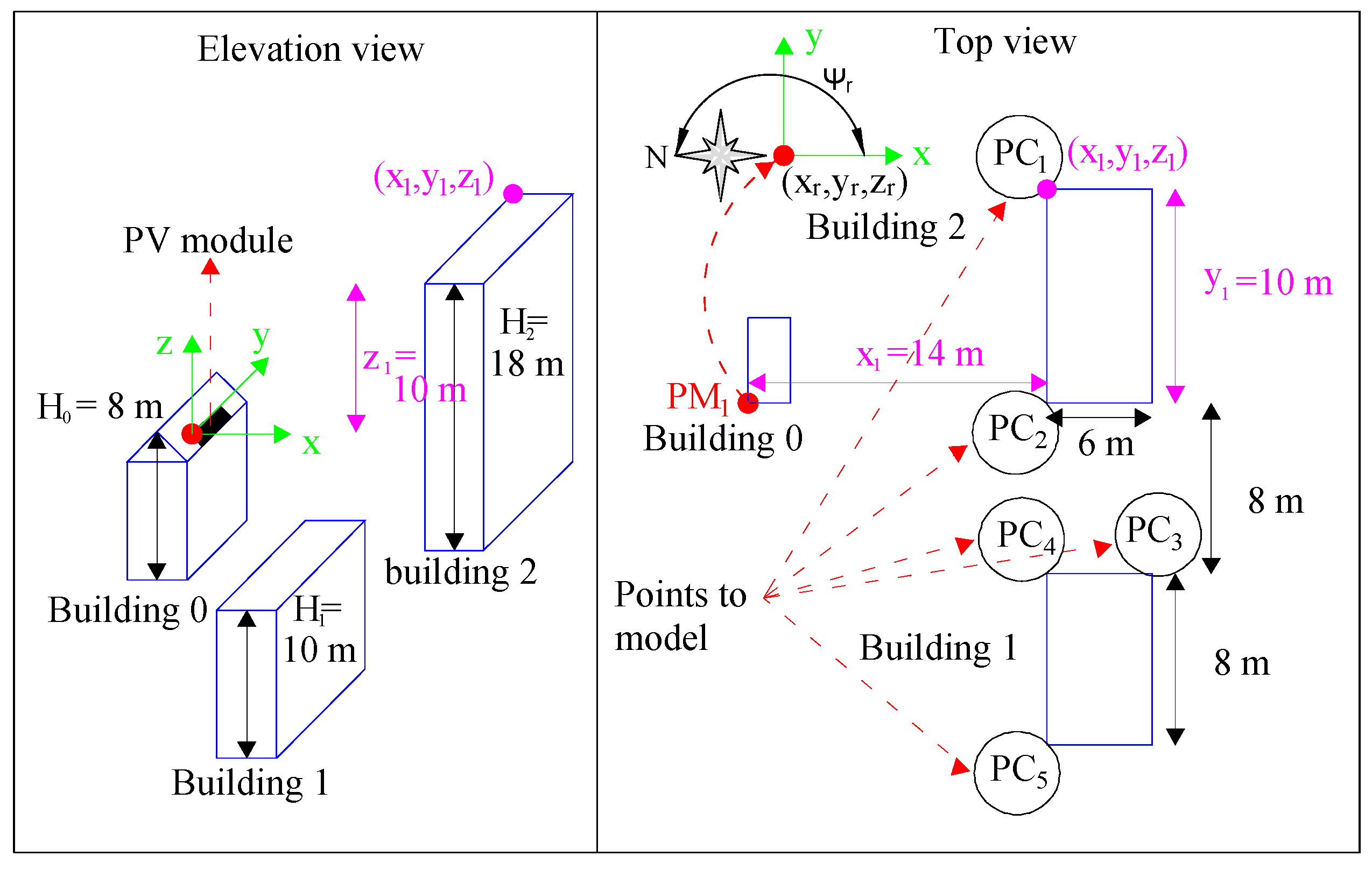
The example proposed in [21] is used to illustrate this procedure. Such an example corresponds to a PVM installed on the roof of a building located in the geographical location described in the previous section (Stuttgart, Germany), where the PVM is represented as a single point in the space ($P{M}_1$). The geometry of the module location and of nearby objects that can cast shadows is illustrated in Figure 3. In this example, two nearby buildings with higher heights can cast shadows on the PVM at certain times of the day and at certain days of the year.

The first step is to identify the key points of the nearby objects ($PCs$) that cast shadows on the module. In Figure 3, the nearby buildings are represented with the key points $P{C}_1$ to $P{C}_5$. These points correspond to the highest corners of the buildings that are in the PVM line of sight. Therefore, with these points, it is possible to represent the contour of the objects that can cast shadows on the PVM.

Once the key points ($P{C}_1$–$P{C}_5$) are identified, it is necessary to define the origin $(x_r,y_r,z_r)$ of a Cartesian coordinate system $x,y,z$ in the floor plan. In the example, the origin is located at $P{M}_1$. The direction of the x-axis must be aligned with one side of the PVM; however, the angle between the positive part of the x-axis and the north (${\mathrm{\Psi }}_r$) must be measured taking into account that $-{180}^{°}<{\mathrm{\Psi }}_r<180$°.

Then, it is necessary to take the following measures for each PC with respect to $(x_r,y_r,z_r)$: the coordinate on the x-axis of the $P{C}_i$ ($x_i$) in [m], the coordinate on the y-axis of the $P{C}_i$ ($y_i$) in [m], and the coordinate on the z-axis of the $P{C}_i$ ($z_i$) in [m], where $i\in [1,\cdots ,5]$ for the example of Figure 3. Such a figure also shows the $x,y,z$ axes, the angle ${\mathrm{\Psi }}_r=180$°, and the coordinate of $P{C}_1$ $(x_1,y_1,z_1)=(14,10,10)$ with respect to $(x_r,y_r,z_r)$.

Next, the azimuth angle (${\gamma }_o$) and the elevation (${\alpha }_0$) must be calculated for each PC using Equations (13) and (14), which are proposed in this paper and based on [21]. For example, for the $P{C}_1$ of Figure 3, $({\gamma }_o,{\alpha }_0)=$ (144.46°, 30.16°); therefore, this point can be represented in the plane E-A of solar paths. Then, this procedure is repeated to represent every PC in the E-A plane of the solar paths, and the PCs are joined with straight lines (linear extrapolation) to create the shading contour in the E-A plane generated by the surrounding objects seen from the point $P{M}_1$. 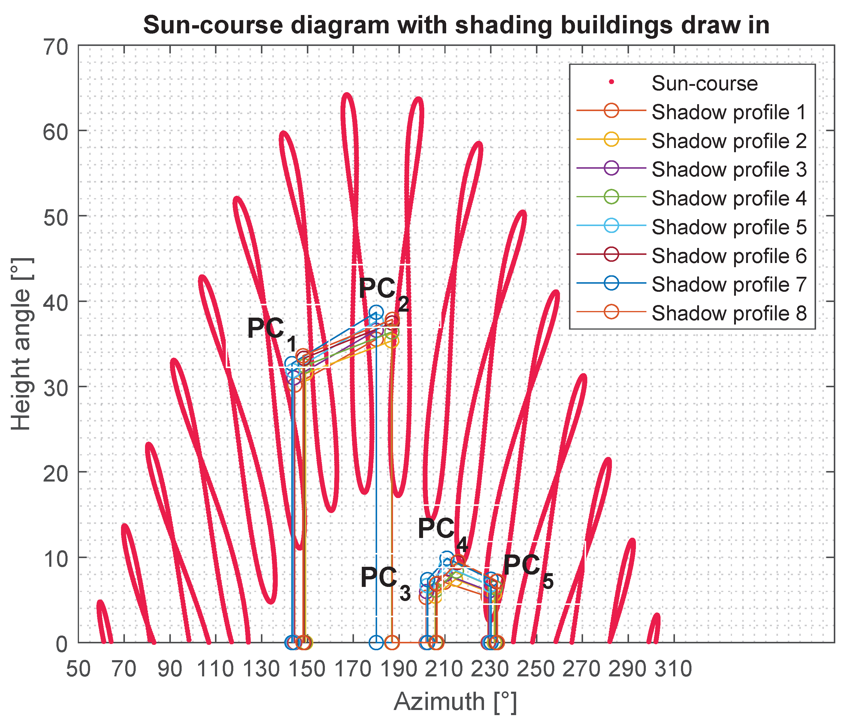Figure 4 shows the shading contour generated by the five key points of the example shown in Figure 3.

$$\begin{array}{c}\hfill {\gamma }_o={\mathrm{\Psi }}_r-{tan}^{-1}\left(\frac{y_i}{x_i}\right)\end{array}$$

(13)

$$\begin{array}{c}\hfill {\alpha }_0={tan}^{-1}\left(\frac{z_i}{\sqrt{{\left(x_i\right)}^2+{\left(y_i\right)}^2}}\right)\end{array}$$

(14)

According to the methodology proposed in [21], the points of the solar paths that are within the shading contour represent the hours at which nearby objects block the direct rays of the sun that exclusively reach the point $P{M}_1$ located in the position $(x_r,y_r,z_r)$. Therefore, it is not possible to adequately determine whether shadows are cast on the PVM or on a particular submodule; in other words, based on the methodology proposed in [21], it can only be estimated if there is a shadow cast at one hour of the year at the point $P{M}_1$.

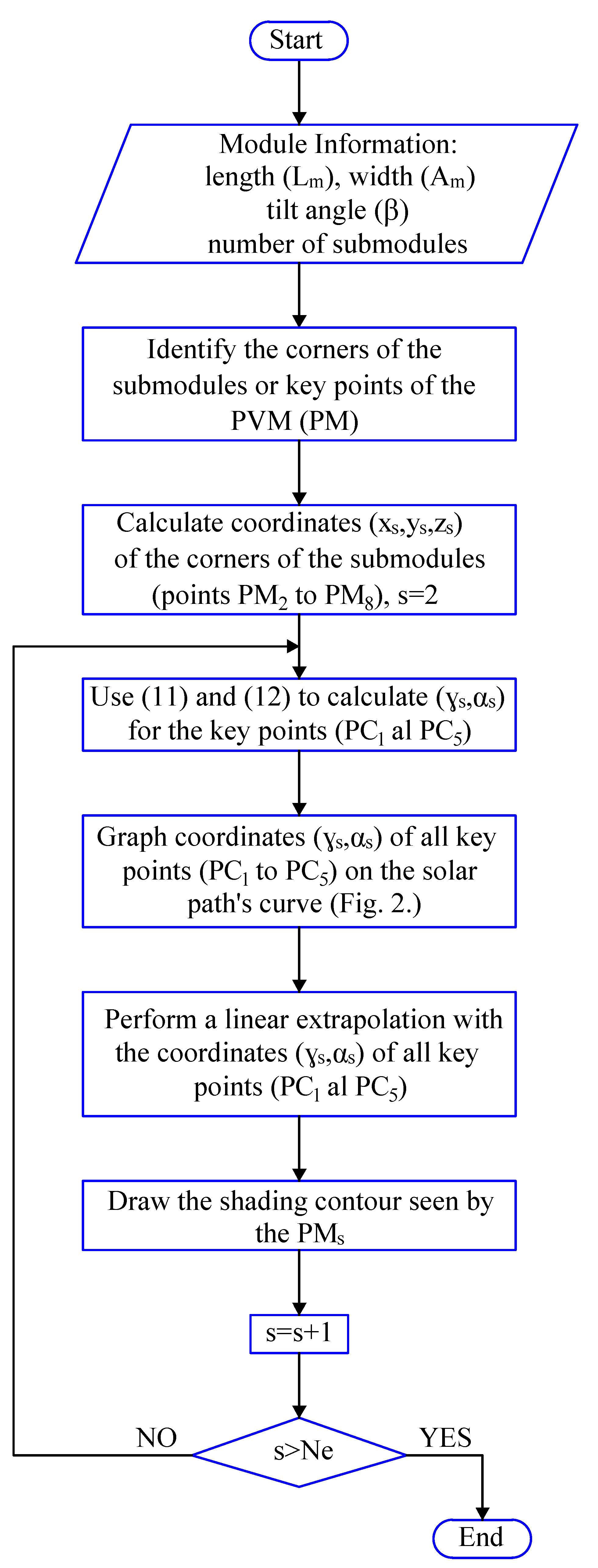
3.3. Extrapolation of the Shading Contours for the Key Points of the PVM

This subsection proposes a procedure used to estimate the shading contours for the points corresponding to the corners of the submodules ($PMs$) by using the shading contour calculated in the previous section or the point $P{M}_1$. Moreover, from those contours, it is estimated which submodules are partially shaded at a given time instant. This procedure is described in the flowchart of Figure 5, which is applied to the example presented in Section 3.1 to illustrate the procedure.

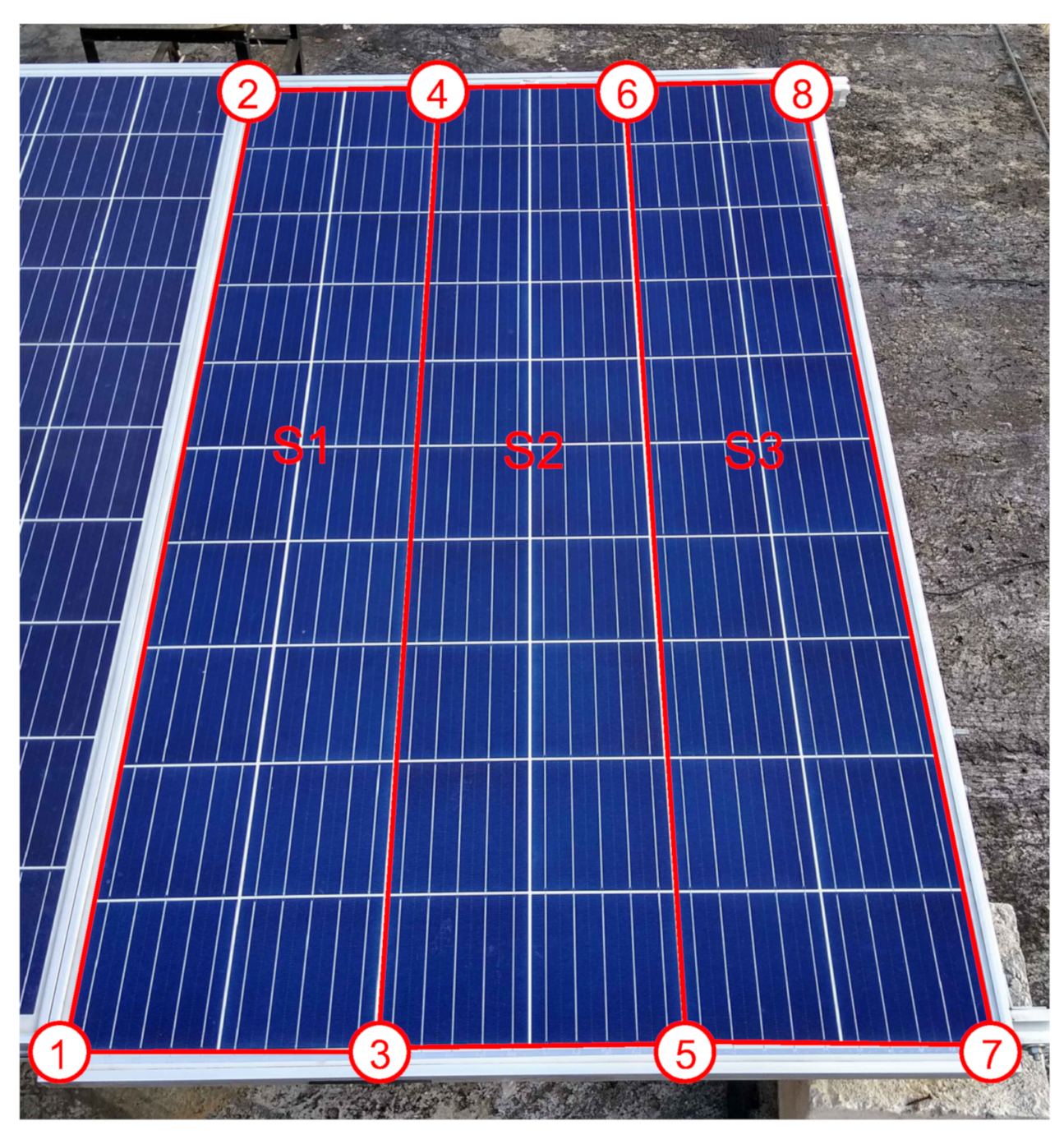
The first step is to obtain the basic information of the module: length ($L_m$) in [m], width ($A_m$) in [m], the angle of inclination ($\beta$) in [°], and the number of submodules of the PVM. As an example, Figure 6 shows a PVM with $L_m=1.65$ [m], $A_m=0.95$ [m], $\beta =48.8$°, and 60 cells grouped into three submodules ($S1$, $S2$, and $S3$) [33].

Then, the key points of the module ($P{M}_s$) that correspond to the total number of the corners of the submodules ($Ne$) must be identified. In the example, there are eight key points ($P{M}_1$ to $P{M}_8$) as shown in Figure 6.

The next step is to calculate the coordinates $(x_s,y_s,z_s)$ of each corner of the submodules on the reference axis $(x,y,z)$, whose origin is the location of $P{M}_1$ $(x_r,y_r,z_r)$. The calculation of $x_s$, $y_s$, and $z_s$ of a PM depends on its location and the geometry of both the module and submodules.

Table 1. Location of $P{M}_1$ to $P{M}_8$ for the example.

Point (${\mathit{x}}_{\mathit{s}}$, ${\mathit{y}}_{\mathit{s}}$, ${\mathit{z}}_{\mathit{s}}$) with Respect to (${\mathit{x}}_{\mathit{r}}$, ${\mathit{y}}_{\mathit{r}}$, ${\mathit{z}}_{\mathit{r}}$) in [m]
$P{M}_2$	(0, $L_m$, 0)
$P{M}_3$	$\left(\frac{A_m}{3}cos\left(\beta \right),0,-\frac{A_m}{3}sin\left(\beta \right)\right)$
$P{M}_4$	$\left(\frac{A_m}{3}cos\left(\beta \right),L_m,-\frac{A_m}{3}sin\left(\beta \right)\right)$
$P{M}_5$	$\left(\frac{2A_m}{3}cos\left(\beta \right),0,-\frac{2A_m}{3}sin\left(\beta \right)\right)$
$P{M}_6$	$\left(\frac{2A_m}{3}cos\left(\beta \right),L_m,-\frac{2A_m}{3}sin\left(\beta \right)\right)$
$P{M}_7$	$\left(A_{m}cos\left(\beta \right),0,-A_{m}sin\left(\beta \right)\right)$
$P{M}_8$	$\left(A_{m}cos\left(\beta \right),L_m,-A_{m}sin\left(\beta \right)\right)$

shows the location of $P{M}_2$–$P{M}_8$ with respect to ($x_r$,$y_r$,$z_r$), which are obtained by analyzing the geometry of the PVM and its submodules as described in Figure 7. It is worth noting that the x-axis of the reference $(x,y,z)$ is parallel to a horizontal plane at a tangent to the surface of the Earth; this is why $beta$ is included in the calculations introduced in Table 1.

Now, a PM ($P{M}_2$) is selected to calculate the shading contour produced by nearby objects regarding this point. Therefore, it is required to calculate the azimuth (${\gamma }_s$) and elevation (${\alpha }_s$) angles for each PC of nearby objects with respect to $P{M}_2$. These angles are calculated using (15) and (16), where $(x_i,y_i,z_i)$ are the coordinates of the point $P{C}_i$ with respect to the origin $(x_r,y_r,z_r)$, previously defined in Section 3.1.

$$\begin{array}{c}\hfill {\gamma }_s={\mathrm{\Psi }}_r-{tan}^{-1}\left(\frac{y_i-y_s}{x_i-x_s}\right)\end{array}$$

(15)

$$\begin{array}{c}\hfill {\alpha }_s={tan}^{-1}\left(\frac{z_i-z_s}{\sqrt{{\left(x_i-x_s\right)}^2+{\left(y_i-y_s\right)}^2}}\right)\end{array}$$

(16)

For the example, there are five $PCs$ (i.e., $i\in [1,\cdots ,5]$) for $P{M}_1$ as explained in Section 3.2; then, it is necessary to calculate the five points on the E-A plane regarding $P{M}_2$: for $P{C}_1$, $({\gamma }_s,{\alpha }_s)=$ (149.2°, 31.5°), for $P{C}_2$, $({\gamma }_s,{\alpha }_s)=$ (186.72°, 35.4°), for $P{C}_3$, $({\gamma }_s,{\alpha }_s)=$ (205.8°, 5.4°), for $P{C}_4$, $({\gamma }_s,{\alpha }_s)=$ (214.6°, 7.4°), and, for $P{C}_5$, $({\gamma }_s,{\alpha }_s)=$ (231.6°, 5.7°).

The coordinates $({\gamma }_s,{\alpha }_s)$ of each PC can be plotted on the E-A plane of the solar paths and joined with straight lines (linear interpolation) to obtain the shading contour of the surrounding objects for $P{M}_2$. Then, the following PM is selected to calculate the shading contour for that point by repeating the procedure described for $P{M}_2$. This process is repeated until the shading contours for all of the PMs of the module have been obtained. Figure 8 shows the shading contours generated by the five key points of the example shown in Figure 3, which affect the eight corners of the submodules.

A zoom into the shading contours of the eight $PMs$ in the example is illustrated in Figure 9. In this figure, the points of the solar paths that are within the shading contours represent the hours at which nearby objects block the direct rays of the sun. In addition, if, within one hour, the solar path is within the shading contour of at least one of the corners of a submodule (e.g., $P{M}_1$, $P{M}_2$, $P{M}_3$, or $P{M}_4$ for submodule 1), then it is assumed that the submodule 1 ($S1$) is shaded. In this way, it is possible to determine, for each submodule, the hours of the year in which the direct rays of the sun are obstructed by nearby objects. Therefore, it is assumed that, during those hours, the submodule only receives diffuse and reflected irradiance and not direct irradiance.

From the proposed methodology, it is possible to detect if there is a shadow (or not) covering a module, a submodule, or even a cell of a PV array if the number of PMs in the PVM is increased, i.e., if the resolution is increased. In this paper, determining the shading at the submodule level is proposed, considering both the inclination angle ($\beta$) and any orientation of the PVM with respect to the north ($\mathrm{\Psi }$).

3.4. Estimation of Shading Factors

As described in Section 2, the model used in this paper requires a vector with the shading factors of each submodule of the PVM ($F_{SV}$) to generate a P-V curve for a given operating condition. Hence, in order to estimate the annual power profile hour by hour, it is necessary to calculate $F_{SV}$ for each hour of the year.

According to the PVM model for a submodule operating under partial shading conditions, the shading factor of a submodule ($F_S$) can be defined as a reduction factor that multiplies $I_{ph}$. In the single-diode PV model, this current is considered as approximately equal to $I_{sc}$ (short-circuit current) for any operating condition ($I_{ph}\simeq I_{sc}$) [31]. Therefore, $F_S$ can be defined as $F_S=I_{sc}∕I_{scn}$, where $I_{scn}$ is the short-circuit current of the submodule without any shadow. However, in order to estimate the power of a PVM, the irradiance data obtained from the evaluation of the solar resource are generally available, but not the values of $I_{sc}$ and $I_{scn}$. Therefore, $F_S$ is defined as shown in (17), where $F_S=1$ when the submodule is not shaded; and a shaded submodule has $F_S=G_{di}/G_g\simeq (G_g-G_d)/G_g=1-G_d/G_g$, where $G_{di}$, $G_d$, and $G_g$ are the diffuse, direct, and global irradiance, respectively. It is worth noting that the last definition of $F_S$ only requires $G_d$ and $G_g$, which are commonly available in the solar resource databases (e.g., [34]).

$$\begin{array}{c}\hfill F_S=\left\{\begin{array}{cc}1& \mathrm{if}\mathrm{submodule}\mathrm{is}\mathrm{unshaded}\hfill \\ 1-\frac{G_d}{G_g}& \mathrm{if}\mathrm{submodule}\mathrm{is}\mathrm{shaded}\hfill \end{array}\right.\end{array}$$

(17)

It is important to clarify that the estimation of $F_S$ assumes that, if a cell of the submodule is completely shaded, the power generation of the entire submodule is reduced by $F_S$ [1,35,36]. Therefore, if, within one hour, it is considered that one corner of a submodule is shaded (according to the methodology of Section 3.3), then it is assumed that at least one cell has been completely shaded; consequently, the $F_S$ value of such a submodule is calculated by using (17).

3.5. Power and Energy Calculation

The first step is to calculate the P-V curves of the module for each hour of the year using the model proposed in [32]. Each curve was calculated using voltage steps of 1 [V] to identify the global maximum power point ($GMPP$), which was taken as the maximum power that the module can generate in each hour. Under conventional operation conditions, such a $GMPP$ is detected using maximum power point tracking (MPPT) algorithms designed for partial shading conditions. Some examples are the MPPT algorithm based on the Harris–Hawk optimization reported in [37], and the MPPT solution based on the slime-mold algorithm reported in [38]; both of them ensure the operation of the PV module at the $GMPP$, even with the existence of multiple local MPPs (LMPP).

Figure 10 shows an example of the PV curve of a PVM with three submodules exposed to $F_{SV}=\left[0.250.750.5\right]$, $G_g=1000$ [W/m${}^2$] and $T_a=25$ [°C]. In the P-V curve, three MPPs are identified, where two LMPPs and the GMPP are observed. It is important to clarify that this curve is valid in an instant of time where $F_{SV}$, $G_g$, and $T_a$ remain constant. However, for the estimation of the energy produced by the PVM, it is assumed that the curve is valid for one hour (time resolution of the analysis).

After identifying the GMPP of the P-V curve calculated for each hour, a power-time (P-t) curve was constructed by plotting the GMPP of each hour of the year. Finally, from such a curve, the energy produced by the module could be estimated as the area under the P-t curve.

4. Simulation Results

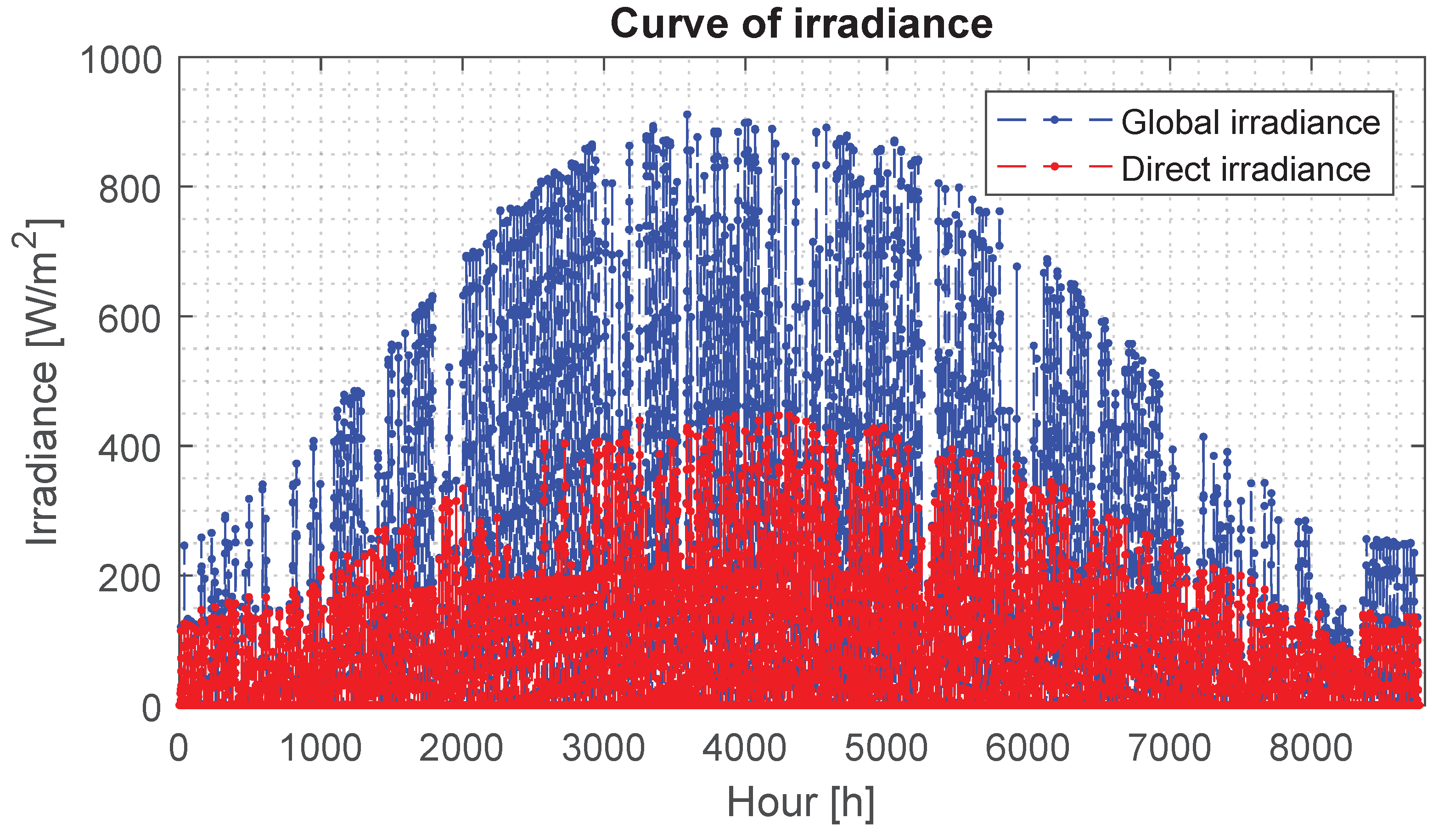
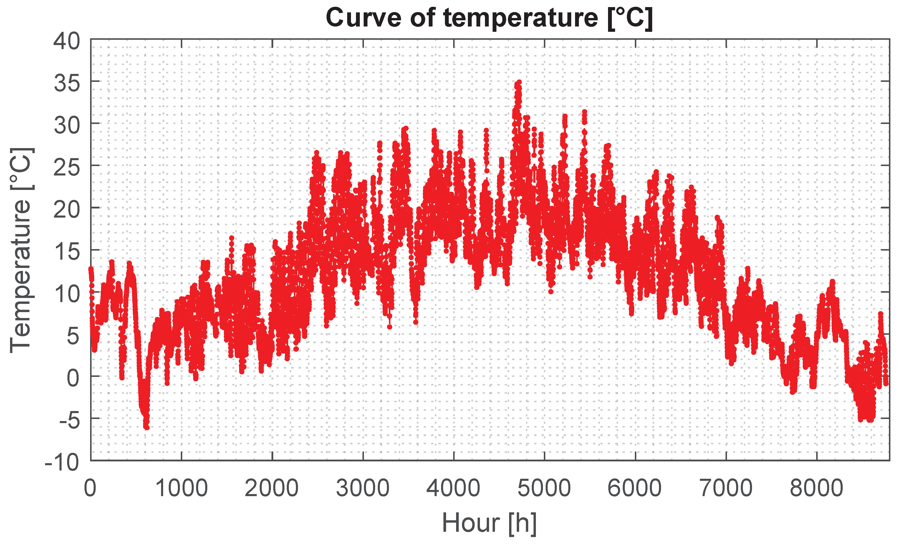
The case study considers the PVM presented in Section 3.1 [21], which is described by the geometry of Figure 3 and located in the city of Stuttgart, Germany ($\varphi =48.8$°, $L_{local}=9.2$°, $L_{zone}=15$°). The irradiance profile (global and direct) and the temperature are shown in Figure 11 and Figure 12, respectively, which were obtained from a public database [34]. The PVM used is the Trinasolar TSM-270PD05 polycrystalline-Si PVM [33], which consists of 60 cells grouped into three submodules as shown in Figure 6, with the following characteristics in STC: power in MPP $P_{mpp}=270$ [W], voltage in MPP $V_{mpp}=30.9$ [V], current in MPP $I_{mpp}=8.73$ [A], open circuit voltage $V_{oc}=37.9$ [V], short-circuit current $I_{sc}=9.22$ [A], nominal efficiency $\eta =16.5$ [%], and $I_{sc}$ temperature coefficient ${\alpha }_{Isc}=0.05$ [%/K].

The single-diode model parameters of each submodule were calculated by using the procedure proposed in [39] from the datasheet STC characteristics of the PVM, obtaining the following values: $I_{sat}=237.82$ [$\mathsf{\mu }$A], $\eta =1.097$, $Rs=0.088$ [$\mathsf{\Omega }$], $Rh=246.670$ [$\mathsf{\Omega }$]. The bypass diode parameters were calculated from the datasheet information, obtaining the following values: $I_{sat,bd}=851.54$ [$\mathsf{\mu }$A] and ${\eta }_{bd}=1.634$.

The power profiles generated with the proposed procedure (red data), and neglecting the partial shading conditions (blue data), are shown in Figure 13. In such a figure, it is observed that there are some hours where the power estimated with the proposed procedure is significantly lower than the power estimated without considering partial shading.

The estimated energy of the PVM, considering and neglecting the partial shading conditions, is 249.83 [kWh] and 263.56 [kWh], respectively. Therefore, neglecting the partial shading in this example causes an energy overestimation equal to 5.21%.

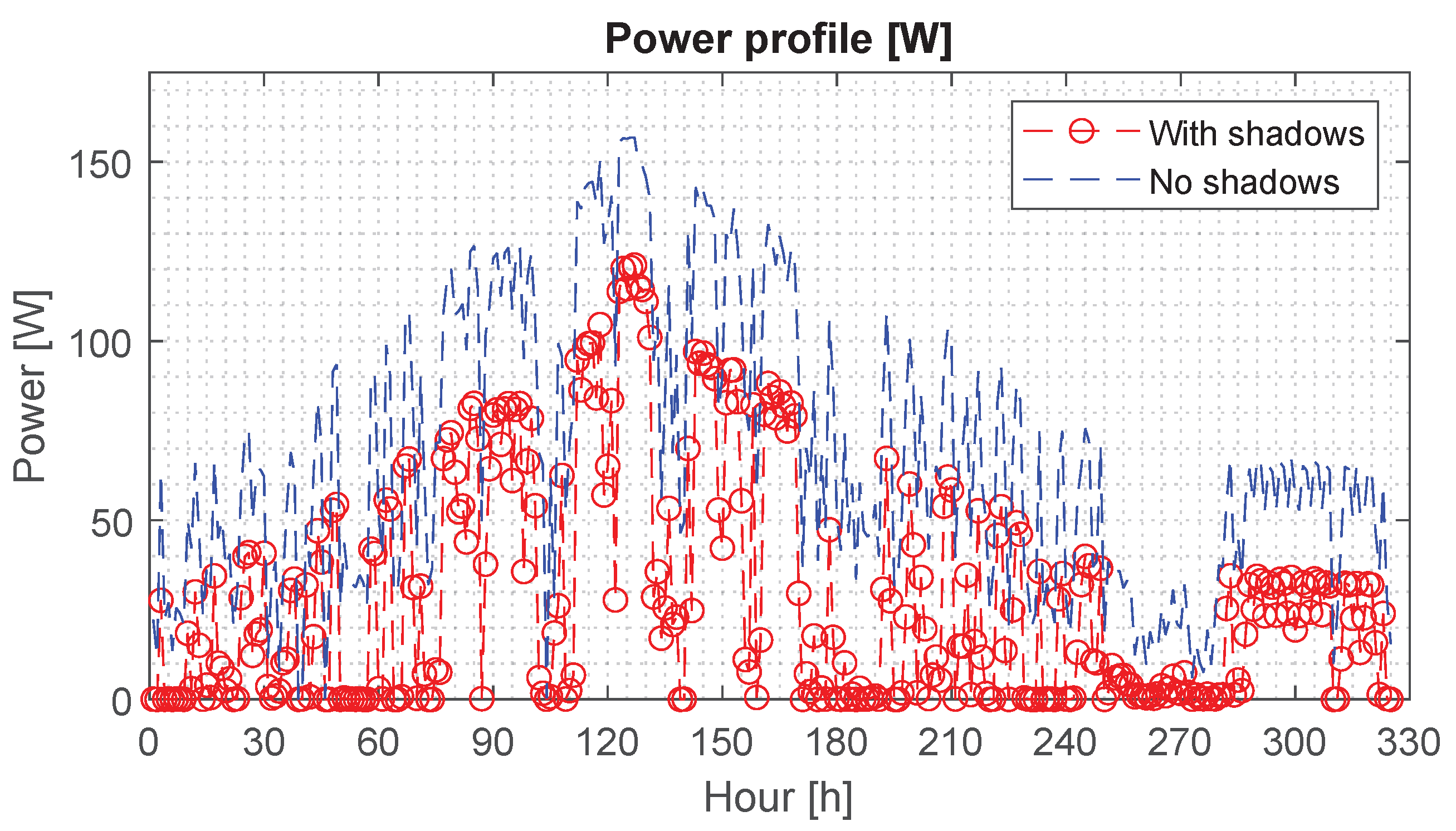
To illustrate the differences in the estimated power, with and without considering partial shading, Figure 14 shows the power profile with one, two, or three shaded submodules for 330 h. In such a figure, the blue color is the power generated when there are shadows on the PVM, whereas the red color is the power generated for the same hours without considering the shadows on the PVM. The figure confirms that significant power losses at different hours occur; these losses are between 0.23% and 99.99% depending on the hour.

Considering only the hours in which there is shade on the PVM, the energy estimated with the proposed procedure is 9.40 [kWh]. In the same hours, without considering the shadows, there is an energy generation of 21.89 [kWh], which corresponds to 57.06% of energy losses per year due to the shading conditions. Therefore, the energy overestimation increases depending on the number of hours of the year when the PVM is operating under partial shading conditions.

5. Experimental Results

The proposed methodology was experimentally validated for a PV panel located on the rooftop of a building in Bucaramanga, Colombia ($\varphi =7.14$°, $L=-73.12$°, $L_{zone}=-75$°). The PV panel was the same one used for the simulation results; hence, the panel length and width ($L_m=1.65$ [m], $A_m=0.95$ [m]), the number of submodules ($Ne=3$), and the corners of the submodules (see PMs in Figure 9) are the same ones used in Section 3.3. However, the tilt angle of the panel ($\beta =12$°) and its location are different, as presented in Figure 15, which shows the orientation of the PV panel, the location of $P{M}_1$, and the key points of the objects that can cast shadows at the rooftop ($P{C}_1$ to $P{C}_4$). In this case, the panel is tilted over its short side (i.e., the height of $P{M}_1$, $P{M}_3$, $P{M}_5$, and $P{M}_7$ is less than the height of $P{M}_2$, $P{M}_4$, $P{M}_6$, and $P{M}_8$); therefore, the locations of $P{M}_2$–$P{M}_8$ with respect to $P{M}_1$ ($x_r$,$y_r$,$z_r$) are calculated by using the equations shown in

Table 2. Location of $P{M}_1$ to $P{M}_8$ for the experiment.

Point (${\mathit{x}}_{\mathit{s}}$, ${\mathit{y}}_{\mathit{s}}$, ${\mathit{z}}_{\mathit{s}}$) with Respect to (${\mathit{x}}_{\mathit{r}}$, ${\mathit{y}}_{\mathit{r}}$, ${\mathit{z}}_{\mathit{r}}$) in [m]
$P{M}_2$	$\left(0,-L_{m}cos\left(\beta \right),-L_{m}sin\left(\beta \right)\right)$
$P{M}_3$	$\left(-\frac{A_m}{3},0,0\right)$
$P{M}_4$	$\left(-\frac{A_m}{3},-L_{m}cos\left(\beta \right),-L_{m}sin\left(\beta \right)\right)$
$P{M}_5$	$\left(-\frac{2A_m}{3},0,0\right)$
$P{M}_6$	$\left(-\frac{2A_m}{3},-L_{m}cos\left(\beta \right),-L_{m}sin\left(\beta \right)\right)$
$P{M}_7$	$\left(-A_m,0,0\right)$
$P{M}_8$	$\left(-A_m,-L_{m}cos\left(\beta \right),-L_{m}sin\left(\beta \right)\right)$

.

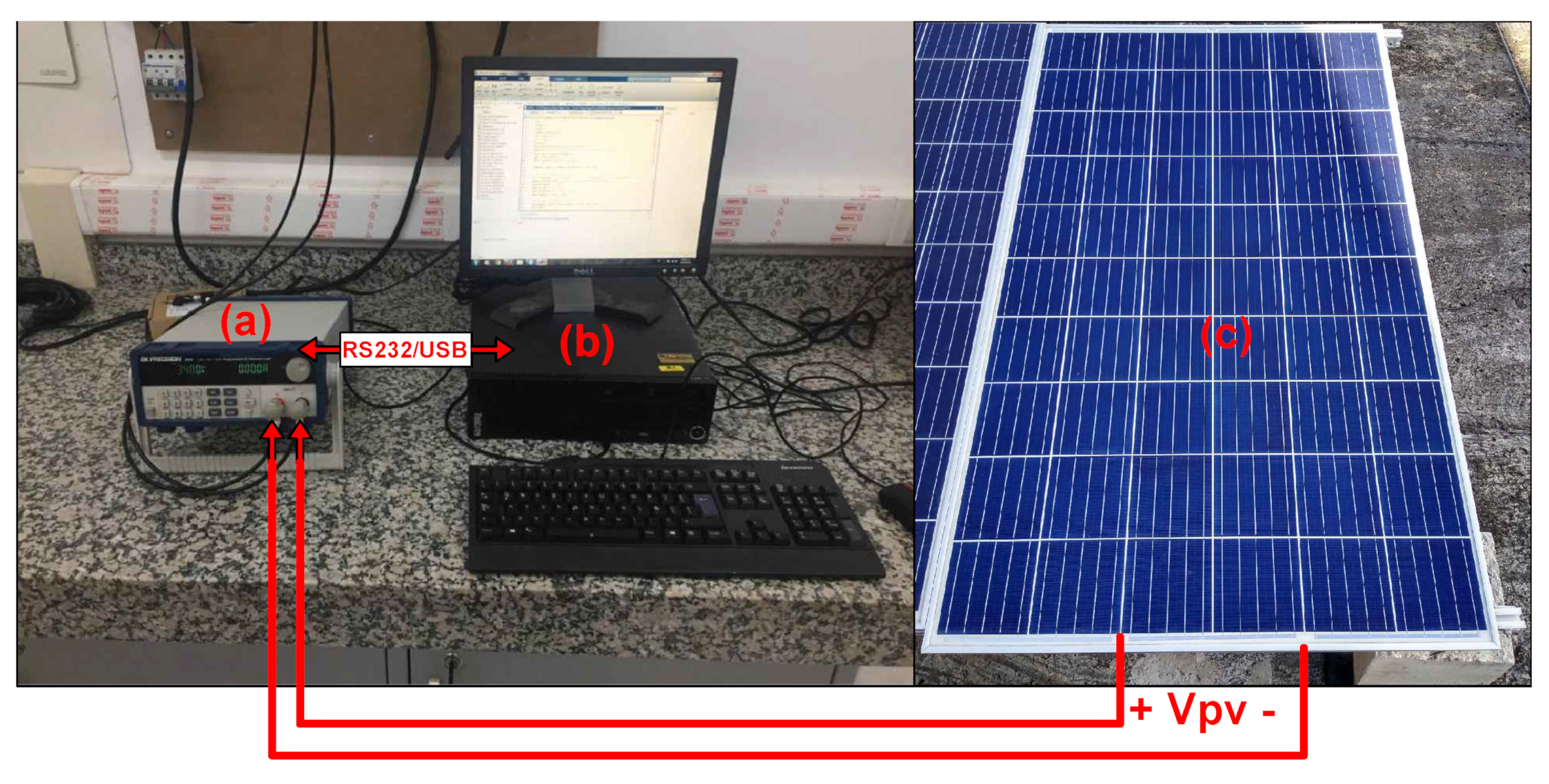
The experimental platform used to measure the PV panel I-V curves is presented in Figure 16. It is formed by a programmable electronic load BK Precision 8500, a PC running Matlab to control the electronic load, and the PV panel. The electronic load and the PV panel are connected through two AWG-12 cables of 30 [m] each; therefore, the total resistance of the cable is $R_{cab}=$ 313.4 [m$\mathsf{\Omega }$]. Such resistance must be considered in the experiment because it is in the range of $R_s$. That is why the voltage measured at the terminals of the PV panel ($V_{pan}$) was calculated as $V_{pan}=V_{el}+R_{cab}·I_{pv}$, where $I_{pv}$ is the measured current of the PV panel and $V_{el}$ is the voltages measured by the electronic load.

The proposed methodology was validated for two time instants of the day to verify its capability in predicting the shaded and unshaded PMs and the P-V curves of the panel. The experiments were carried out on the 17 October 2019 at 15:14 p.m. (Experiment 1, $G=586.5$ [W/m${}^2$], and $T_a=28.3$°) and 15:23 p.m. (Experiment 2, $G=186.5$ [W/m${}^2$], and $T_a=29.3$°) to highlight the significant variability of the shadow cast on the panel and the capacity of the proposed methodology to predict such variability. The estimation of the shaded/unshaded PMs was compared with the ones obtained with the procedure described in [21] (from here on, “reference procedure”), which considers one PM and uniform irradiance for the entire panel. Then, such information was used by the single-diode model to calculate the P-V curve of the reference procedure.

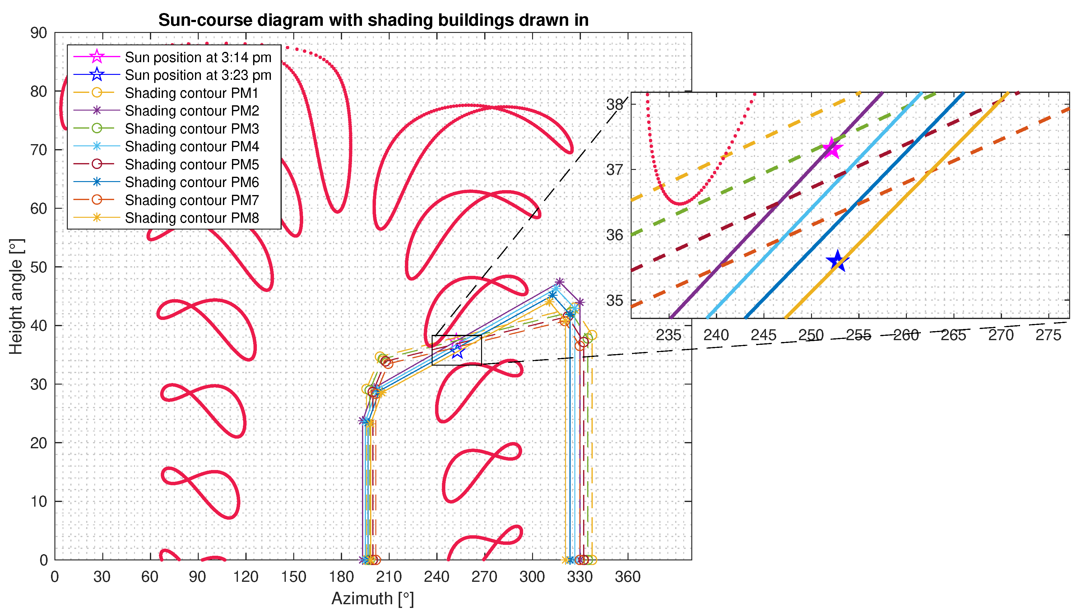
The shading contours of the experiment described in Figure 15 are introduced in Figure 17, as well as the position of the sun for the two time instants considered in the experiments. Additionally, Figure 18 and Figure 19 show a photo of the PV panel to the left and the corresponding P-V curve to the right. Such P-V curves correspond to the experimental measurements and the results obtained with the proposed and reference procedures.

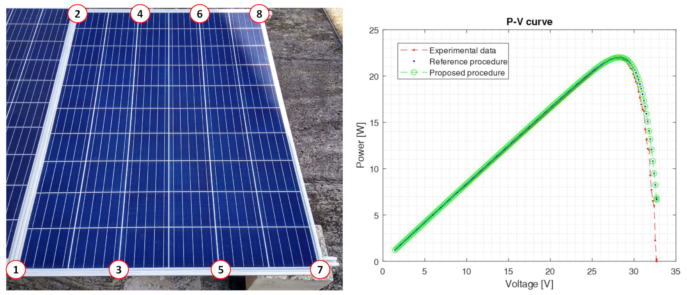
The point in Experiment 1 (3:14 p.m. in Figure 17) is within the shading contours 1, 2, and 3 and out of the shading contours 4, 5, 6, 7, and 8, which agrees with the real operating condition shown at the left of Figure 18. This means that submodules S1 and S2 are shaded whereas submodule S3 is unshaded. Further, from the experimental measurements, it can be defined that $I_{ph}\approx I_{scn}=5.486$ [A] and $I_{sc}=0.813$ [A]; then, $F_{sv}=\left[F_{S1}{F}_{S2}1.0\right]$, where $F_{S1}=F_{S2}=I_{sc}/I_{scn}=0.813/5.486=0.1482$. Then, using the model proposed in [32], it is possible to obtain the P-V curves shown at the right of Figure 18. These curves show that the proposed procedure correctly identifies the shaded and unshaded submodules, reproduces the P-V curve, and estimates the GMPP with an error of $2.907[\%]$; whereas the reference procedure underestimates the power generation with an error of $-54.298[\%]$. These results were obtained with the following single-diode model parameters: $I_{sat}=1.549$ [nA], $\eta =0.972$, $Rs=0.175$ [$\mathrm{\Omega }$], $Rh=400.804$ [$\mathrm{\Omega }$], $I_{sat,bd}=425.77$ [$\mathsf{\mu }$A], and ${\eta }_{bd}=0.6783$.

Similarly, the location of the point in Experiment 2 in Figure 17 (3:23 p.m.) indicates that only $P{M}_8$ is unshaded, whereas the other PMs are shaded, which coincides with the photo at the left of Figure 19. In this case, all of the submodules are shaded; hence, it is assumed that $I_{ph}$ of each module corresponds to the short-circuit current of the PV panel, i.e., $I_{ph}\approx I_{scn}=0.846$ [A] and $F_{sv}=\left[1.01.01.0\right]$. The experimental P-V curves and the ones obtained with the proposed and reference methods are presented at the right of Figure 19. For this case, the P-V curves obtained with proposed and reference methods are the same since all the submodules are shaded, which results in a single MPP. Additionally, the MPP is estimated with an error of $-0.121[\%]$. These results were obtained with the same single-diode model parameters of the first experiment, with the exception of $I_{sat}$ ($I_{sat}=0.3098$ [nA]), which is expected due to its temperature dependency.

These results show that the proposed method improves the accuracy of the estimation power production of a PV panel considering the partial shadings generated by surrounding objects, since neglecting the shadows cast on the PV panel can be translated into a significant underestimation or overestimation of the power produced by a PV panel.

6. Conclusions

This paper has presented a procedure based on the single-diode model used to estimate the power losses caused by partial shading conditions. The proposed methodology allows for a consideration of the spatial location of the PVM, including the angle of inclination. Moreover, this paper presents a suitable alternative for the calculation of shading factors, which requires using the PVM model operating under partial shading conditions. Finally, the proposed methodology allows for the direct estimation of the generated power, the generated energy, and the energy losses of a PVM with high precision since an accurate PVM model is used. The proposed approach is useful for sizing PV systems, and, in turn, enables us to evaluate the feasibility of installing a PVM in a particular location.

The simulation and experimental results demonstrated that the power losses caused by shading conditions are not negligible; hence, these losses should be accurately calculated to improve the feasibility analysis. Finally, increasing the granularity of the model and number of PMs will increase the estimation accuracy, but, at the same time, the computational effort will also be increased.