Mathematical Models and Nonlinear Optimization in Continuous Maximum Coverage Location Problem

Abstract

This paper considers the maximum coverage location problem (MCLP) in a continuous formulation. It is assumed that the coverage domain and the family of geometric objects of arbitrary shape are specified. It is necessary to find such a location of geometric objects to cover the greatest possible amount of the domain. A mathematical model of MCLP is proposed in the form of an unconstrained nonlinear optimization problem. Python computational geometry packages were used to calculate the area of partial coverage domain. Many experiments were carried out which made it possible to describe the statistical dependence of the area calculation time of coverage domain on the number of covering objects. To obtain a local solution, the BFGS method with first-order differences was used. An approach to the numerical estimation of the objective function gradient is proposed, which significantly reduces computational costs, which is confirmed experimentally. The proposed approach is shown to solve the maximum coverage problem of a rectangular area by a family of ellipses.

1. Introduction

The maximum coverage problem is a classical problem in computer science, computational complexity theory, and operations research. In the original formulation, the problem is as follows.

There are a family of sets $\mathsf{\Omega }=\left\{{\mathrm{S}}_1,\dots ,{\mathrm{S}}_{\mathrm{n}}\right\}$ and integer number $1\le \mathrm{k}\le \mathrm{n}$. Sets may have some elements in common. The objective is to find such a family $\tilde{\mathsf{\Omega }}\subseteq \mathsf{\Omega }$ of $\mathrm{k}$ sets from $\mathsf{\Omega }$ so that the maximum number of elements is covered, i.e., the union ${\displaystyle \underset{{\mathrm{S}}_{\mathrm{i}}\subseteq \tilde{\mathsf{\Omega }}}{\cup }{\mathrm{S}}_{\mathrm{i}}}$ of the selected sets has the maximum size.

The great interest of scientists in the problem of maximum coverage is associated with a wide range of its practical applications. The concept of coverage is associated with video surveillance cameras, emergency warning systems, mobile communications and the Internet, radio stations, environmental sensors, service systems, etc. This leads to the need to cover certain areas and is associated with an analysis of the location of objects of various nature. A major category of location analysis approaches involves coverage when an entity provides services based on spatial proximity. This may be based on travel time, line-of-sight, or hearing factors. These spatial footprints reflect services and may be regular or irregular, contiguous, or fragmented in area. One of the most common approaches to location modeling is the maximum coverage location problem (MCLP). Such a problem is the subject of study for both operations research theory and computational geometry. In this case, the goal is to place several objects in a given region in such a way as to maximize (minimize) some objective function associated with the considered type of objects.

In most of these problems, a demand point is considered to be covered by a facility if the distance or travel time between them is less than a given predetermined value. It is desirable that all points of demand are served by at least one enterprise. However, often full coverage of demand in the region is impossible due to restrictions on the possible number of objects to be placed. In this case, the task is to cover the maximum possible area of demand through the efficient use of limited resources.

Note that the problems associated with determining the location of objects are both discrete and continuous in nature. In the discrete case, there is a finite set of possible locations of potential objects, and it is required to choose their optimal location. Such tasks arise in the placement of physical services, when it is possible to predetermine a finite set of admissible locations. At the same time, there is a wide class of problems when it is allowed to place objects in the entire space or its continual subdomain. Such tasks are continuous (for example, in telecommunications networks, when placing sensors or radar stations, etc.). In this case, continuity conditions can be imposed not only on the sets of admissible locations, but also on the service area. This article is devoted to mathematical modeling and solving these coverage optimization problems.

2. Background

Reviews [1,2,3,4,5] are devoted to the issues of object location analysis based on the modeling of coverage problems. The main approaches to location analysis consider coverage in the sense that an object provides services within spatial proximity, i.e., each object has a spatial footprint that defines a service area. Article [6] provides extended overview of the maximal covering location problem, highlighting the use, application, solution, evolution, and generalization of this important location analytic approach.

The problem of placing a certain number of objects within an acceptable service distance to maximize demand in a given region was posed and formalized by Church and ReVelle [7]. This problem is called the maximum coverage location problem (MCLP). To solve this problem, two sets of discrete locations were considered, representing demand and possible locations. As a result, the MCLP is formulated as an integer linear programming problem that can be solved in various ways. Variations arise due to the use of different methods for determining the area of coverage of a potential object or assigning weights to sites on several factors and parameters.

The standard form of MCLP considers a finite set of potential locations for objects, and a set of discrete points represents demand. The paper [8] proposes a generalization that allows both facilities and demand points to be placed continuously on a plane. Such a problem is called planar MCLP. An exact planar MCLP solution, assuming that the need for coverage exists anywhere in the surrounding area and that objects can also be arbitrarily placed in this area, is impossible due to the NP-hard nature of the problem [9]. Several heuristic methods have been proposed in an attempt to obtain acceptable solutions. For example, paper [9] describes a greedy algorithm for MCLP that selects at each step the location containing the largest number of uncovered elements. This greedy algorithm is claimed to be the best approximation algorithm in polynomial time.

In the work [10], a planar MCLP with partial coverage and rectangular demand and service zones is studied. The problem is to position a given number of rectangular service zones on the two-dimensional plane to partially cover a set of existing (possibly overlapping) rectangular demand zones such that the total covered demand is maximized. Based on the properties of the model, the possibility of a significant reduction in the search space is theoretically substantiated and a modification of the branch and bound algorithm for solving the problem is presented. The authors of [10,11] use a computational geometry approach to study partial coverage with rectangular and circular service areas. However, according to [12], optimality is guaranteed only in some special cases.

The paper [13] presents a fuzzy maximally covering location problem in which travel time between any pair of nodes is considered to be a fuzzy variable. A hybrid algorithm of fuzzy simulation and simulated annealing is used to solve MCLP. Some numerical examples are solved and analyzed to show the performance of the proposed algorithm.

In the article [14], a mixed integer non-linear programming model was formulated for distributing the position of a number of rectangular objects of unequal area in a continuum of a planar plant site with a predetermined fixed area. A continuous approach to the problem is taken. Constraints are developed to eliminate the possible overlap between the different facilities. A novel simulated annealing algorithm is developed to solve large instances of the problem. A unique heuristic algorithm is used for initial solution.

We especially note the work [15], in which the continuous setting of MCLP is analyzed. Continuity conditions are imposed on the location of objects, however, the discrete structure of the service domain is preserved, taking into account the graph of relations between enterprises. The problem of mixed integer non-linear programming is formulated. At the same time, taking into account the geometric properties, the authors propose its equivalent reformulation as an integer linear programming problem.

Other approaches use the division of demand into several smaller regions and the ratio between fully covered or uncovered areas [8,16,17,18]. A facility is assumed to cover the demand for a region if it covers the entire region. Partially covered areas are considered as uncovered areas. Such coverage is called binary. Consideration of the binary coverage makes it possible to obtain a finite set of potential service points determined by the set of polygon intersection points. As a result, an integer linear programming problem is formulated. However, although binary coverage makes planar MCLP manageable, this approach is prone to significant errors because all partially covered regions, which may have a significant coverage area, are left out and ignored in the final solution [12].

Note that obtaining even a partial maximum coverage is not trivial. Therefore, as an auxiliary problem, one often considers partial coverage by only one object. In the paper [19], a method for solving the problem of determining the location of a circular service area in a polygonal zone is described based on the calculation of the mean axis of the zone. Taking into account partial coverage, in the work [20] it is proposed to approximate the optimal position of a single circular footprint with bounded error in an unconnected area with holes bounded by line or circle segments. The authors describe an efficient algorithm for accurately calculating the overlap area of a circle and a polygon, and introduce the concept of a coverage map for more information. The paper [21] presents improved algorithms for matching two polygonal shapes to approximate their maximum overlap. The run time of algorithms is studied.

The article [22] describes an approach to solving the problem of locating a disk so that its overlap area with a piecewise circular domain is near-optimal when considering partial coverage. The concept of an overlap area map is introduced. Parallel algorithm on graphics processing units are discussed for calculating the overlap area map and deriving a set of near-optimal locations from the overlap area map. Particular attention is paid to the process of calculating the overlap area. The authors visualize the information obtained, highlighting the optimal location, and analyze the experimental results obtained by implementing the proposed algorithms.

The study [23] presents an approach to the maximum coverage of a polygonal area by disk services of a given radius. Of particular interest is a parallel optimization method using simulated annealing based on a perturbation strategy and a probabilistic estimate of the covered area of a polygon. The system provides in a reasonable run time fairly good location of disks, starting with an arbitrary initial solution. The paper [24] considers the problem of covering compact polygonal set by identical circles of minimal radius. A mathematical model of the problem based on Voronoi polygons is constructed and its characteristics are investigated. A modification of the Zoutendijk feasible directions method is developed to search local minima. A special approach is suggested to choose starting points. Many computational examples are given.

Access to and solution of the MCLP is also possible in GIS software packages. For example, structuring and solving an MCLP application instance in ArcGIS and TransCAD, among others, is easily accomplished. In ArcGIS, there are location-allocation functions in network analyst, and, in particular, ‘‘maximize coverage’’ would enable an MCLP to be set up as the problem type. Similarly, in TransCAD, one would use ‘‘facility location analysis’’ to accomplish this. There are in fact a number of reported application studies that have relied on this basic approach using GIS, such as [25,26]. It is important to note that GIS packages facilitating access to the MCLP typically solve problems using a heuristic [4].

The evolution of the application of MCLP has occurred concurrently in concert with the development, growth, and maturation of GIS. The MCLP access and solution is possible in various GIS software packages. The authors of [3,27] discuss that GIS is a combination of hardware, software, and procedures enabling data management and spatial query. Key components of GIS include data capture, modeling, management, manipulation, analysis, and display. It is important that in addition to generating and working with spatial information, GIS supports a number of analytical functions, many of which facilitate the MCLP specification and application. In the paper [4], the capabilities of a GIS for carrying out suitability analysis, as well as operations associated with containment, overlay, distance, buffering, and spatial interpolation, among others. Much spatial information now exists, expediting coverage location analysis as well.

3. Materials and Methods

3.1. Mathematical Model of Continuous Maximum Coverage Location Problem

Let us formulate the continuous MCLP as a geometric problem. In the space ${\mathrm{R}}^{\mathrm{d}},\hspace{0.33em}\mathrm{d}=2,3$ there are a certain domain ${\mathrm{S}}_0$ and a family of geometric objects $\left\{{\mathrm{S}}_1,\dots ,{\mathrm{S}}_{\mathrm{n}}\right\}$ of a given shapes and sizes. We will say that a family of objects $\left\{{\mathrm{S}}_1,\dots ,{\mathrm{S}}_{\mathrm{n}}\right\}$ covers some subdomain $\tilde{\mathrm{S}}\subseteq {\mathrm{S}}_0$ if each point $\tilde{\mathrm{S}}$ belongs to at least one of the objects of the family. The problem is to find such a location of objects ${\mathrm{S}}_1,\dots ,{\mathrm{S}}_{\mathrm{n}}$ that they cover as much of the domain ${\mathrm{S}}_0$ as possible. ${\mathrm{S}}_0$ is called the coverage domain, and ${\mathrm{S}}_1,\dots ,{\mathrm{S}}_{\mathrm{n}}$—the covering objects.

To formalize the continuous MCLP we make the following notations: ${\mathbf{J}}_{\mathrm{n}}^{}=\left\{1,\dots ,\mathrm{n}\right\}$, ${\mathbf{J}}_{\mathrm{n}}^0={\mathbf{J}}_{\mathrm{n}}^{}\cup \left\{0\right\}=\left\{0,1,\dots ,\mathrm{n}\right\}$. Geometric object ${\mathrm{S}}_{\mathrm{i}}\subset {\mathrm{R}}^{\mathrm{d}},\hspace{0.17em}\mathrm{i}\in {\mathbf{J}}_{\mathrm{n}}^0$ means a geometric set of points $\mathrm{P}\in {\mathrm{R}}^{\mathrm{d}}$ that satisfy inequalities ${\mathrm{f}}_{\mathrm{i}}(\mathrm{P},{\mathbf{m}}^{\mathrm{i}})\ge 0$. The equation ${\mathrm{f}}_{\mathrm{i}}(\mathrm{P},{\mathbf{m}}^{\mathrm{i}})=0$ defines the boundary of the object ${\mathrm{S}}_{\mathrm{i}}$ and determines its shape. In the general case, functions ${\mathrm{f}}_{\mathrm{i}}(\mathrm{P},{\mathbf{m}}^{\mathrm{i}})$, $\mathrm{i}\in {\mathbf{J}}_{\mathrm{n}}^0$ contain constants ${\mathbf{m}}^{\mathrm{i}}=({\mathrm{m}}_1^{\mathrm{i}},\dots ,{\mathrm{m}}_{{\mathsf{\alpha }}_{\mathrm{i}}}^{\mathrm{i}})$, which are called metric parameters of the shape of the object ${\mathrm{S}}_{\mathrm{i}}$. These parameters determine the linear sizes of the corresponding objects.

Consider a fixed Cartesian coordinate system in space ${\mathrm{R}}^{\mathrm{d}},\hspace{0.33em}\mathrm{d}=2,\hspace{0.17em}3$, and with each object ${\mathrm{S}}_{\mathrm{i}}\subset {\mathrm{R}}^{\mathrm{d}},\hspace{0.17em}\mathrm{i}\in {\mathbf{J}}_{\mathrm{n}}^0$, connects own coordinate system, the beginning of which is called the pole of this object. The relative position of these system will be characterized by parameters ${\mathbf{p}}^{\mathrm{i}}=({\mathrm{p}}_1^{\mathrm{i}},\dots ,{\mathrm{p}}_{{\mathsf{\beta }}_{\mathrm{i}}}^{\mathrm{i}})=({\mathbf{v}}^{\mathrm{i}},{\mathsf{\theta }}^{\mathrm{i}}),\hspace{0.33em}\mathrm{i}\in {\mathbf{J}}_{\mathrm{n}}^0$, where ${\mathbf{v}}^{\mathrm{i}}$—a coordinate vector of the pole of the object ${\mathrm{S}}_{\mathrm{i}}$ in a fixed coordinate system, and ${\mathsf{\theta }}^{\mathrm{i}}$—a vector of angular parameters that determine the relative position of the axes of own and fixed coordinate systems. The coordinates of the vector ${\mathbf{p}}^{\mathrm{i}}=({\mathrm{p}}_1^{\mathrm{i}},\dots ,{\mathrm{p}}_{{\mathsf{\beta }}_{\mathrm{i}}}^{\mathrm{i}})$ indicates the position of the object ${\mathrm{S}}_{\mathrm{i}}$ in ${\mathrm{R}}^{\mathrm{d}},\hspace{0.33em}\mathrm{d}=2,3$ and are called placement parameters. In this case, the position of the object ${\mathrm{S}}_{\mathrm{i}}$ relative to the fixed coordinate system is given by the equation of the general position, which has the form

$${\mathrm{F}}_{\mathrm{i}}(\mathrm{P},{\mathbf{m}}^{\mathrm{i}},{\mathbf{v}}^{\mathrm{i}},{\mathsf{\theta }}^{\mathrm{i}})={\mathrm{f}}_{\mathrm{i}}\left(\mathrm{A}(\mathrm{p}-{\mathbf{v}}^{\mathrm{i}}),{\mathbf{m}}^{\mathrm{i}}\right)=0,$$

(1)

where $\mathrm{A}$ is the orthogonal operator expressed through angular parameters ${\mathsf{\theta }}^{\mathrm{i}}$.

In the papers [28,29], methods for constructing configurations of geometric objects are described, and classes of packing, layout, and covering configurations are identified. A configuration space of geometric objects is constructed, the generalized variables of which are placement parameters and metric parameters of objects.

Let us apply these results to build a model of the continuous MCLP. Let $\mathsf{\Omega }=\left\{{\mathrm{S}}_1,\dots ,{\mathrm{S}}_{\mathrm{n}}\right\}$ be a family of geometric objects with metric parameters of the shape ${\mathbf{m}}^{\mathrm{i}}=({\mathrm{m}}_1^{\mathrm{i}},\dots ,{\mathrm{m}}_{{\mathsf{\alpha }}_{\mathrm{i}}}^{\mathrm{i}})$ and placement parameters ${\mathbf{p}}^{\mathrm{i}}=({\mathrm{p}}_1^{\mathrm{i}},\dots ,{\mathrm{p}}_{{\mathsf{\beta }}_{\mathrm{i}}}^{\mathrm{i}})=({\mathbf{v}}^{\mathrm{i}},{\mathsf{\theta }}^{\mathrm{i}}),\hspace{0.33em}\mathrm{i}\in {\mathbf{J}}_{\mathrm{n}}^0$. A parameters ${\mathbf{g}}^{\mathrm{i}}=({\mathbf{m}}^{\mathrm{i}},{\mathbf{p}}^{\mathrm{i}})=({\mathrm{m}}_1^{\mathrm{i}},\dots ,{\mathrm{m}}_{{\mathsf{\alpha }}_{\mathrm{i}}}^{\mathrm{i}},{\mathrm{p}}_1^{\mathrm{i}},\dots ,{\mathrm{p}}_{{\mathsf{\beta }}_{\mathrm{i}}}^{\mathrm{i}})$ is called a generalized variable of the object ${\mathrm{S}}_{\mathrm{i}}$. The dimension of the vector ${\mathbf{g}}^{\mathrm{i}}$ is equal to ${\mathsf{\gamma }}_{\mathrm{i}}={\mathsf{\alpha }}_{\mathrm{i}}+{\mathsf{\beta }}_{\mathrm{i}}$. The object ${\mathrm{S}}_{\mathrm{i}}$ with the generalized variables ${\mathbf{g}}^{\mathrm{i}}$ denote by ${\mathrm{S}}_{\mathrm{i}}({\mathbf{g}}^{\mathrm{i}})$, $\mathrm{i}\in {\mathbf{J}}_{\mathrm{n}}^0$.

Note that, depending on the specifics of the problem, some generalized variables can be fixed. To indicate this we will use a cap over the corresponding variable. In continuous MCLP, placement parameters of the coverage domain ${\mathrm{S}}_0$ are assumed to be fixed and usually equal to ${\widehat{\mathbf{p}}}^0=(0,\dots ,0)$. Metric parameters ${\mathbf{m}}^0$ in the general case are variable, unless otherwise specified by the problem. Considering problems when the sizes of ${\mathrm{S}}_0$ are known, we will assume ${\mathbf{m}}^0={\widehat{\mathbf{m}}}^0$, so ${\widehat{\mathbf{g}}}^0=({\widehat{\mathbf{m}}}^0,{\widehat{\mathbf{p}}}^0)$.

Using set-theoretic operations, we build a complex object

$$\mathsf{\Omega }={\mathrm{S}}_0\cap {\displaystyle \underset{\mathrm{i}=1}{\overset{\mathrm{n}}{\cup }}{\mathrm{S}}_{\mathrm{i}}}.$$

(2)

We assume that Formula (2) determines the structure of a complex object $\mathsf{\Omega }$, i.e., the rule of its formation.

Having determined the generalized variables ${\mathbf{g}}^{\mathrm{i}}$, $\mathrm{i}\in {\mathbf{J}}_{\mathrm{n}}^0$ of the constituent objects ${\mathrm{S}}_{\mathrm{i}}$, we form a parameterized object

$$\mathsf{\Omega }(\mathbf{g})=\mathsf{\Omega }({\widehat{\mathbf{g}}}^0,{\mathbf{g}}^1,\dots ,{\mathbf{g}}^{\mathrm{n}})={\mathrm{S}}_0({\widehat{\mathbf{g}}}^0)\cap {\displaystyle \underset{\mathrm{i}\in {\mathbf{J}}_{\mathrm{n}}}{\cup }{\mathrm{S}}_{\mathrm{i}}({\mathbf{g}}^{\mathrm{i}})}.$$

(3)

In ${\mathrm{R}}^{\mathrm{d}},\hspace{0.33em}\mathrm{d}=2,3$, each fixed vector $\hat{\mathbf{g}}=({\widehat{\mathbf{g}}}^0,{\widehat{\mathbf{g}}}^1,\dots ,{\widehat{\mathbf{g}}}^{\mathrm{n}})$ of generalized variables corresponds to a complex geometric object of a given structure

$$\mathsf{\Omega }(\hat{\mathbf{g}})={\mathrm{S}}_0({\widehat{\mathbf{g}}}^0)\cap {\displaystyle \underset{\mathrm{i}\in {\mathbf{J}}_{\mathrm{n}}}{\cup }{\mathrm{S}}_{\mathrm{i}}({\widehat{\mathbf{g}}}^{\mathrm{i}})}.$$

(4)

Depending on the dimension of ${\mathrm{R}}^{\mathrm{d}},\hspace{0.33em}\mathrm{d}=2,3$, we calculate the measure (area or volume) of the formed object $\mathsf{\Omega }(\hat{\mathbf{g}})$, which we denote by $\mathsf{\mu }\left(\mathsf{\Omega }(\hat{\mathbf{g}})\right)$. Thus, an arbitrary set of generalized variables $\mathbf{g}=({\widehat{\mathbf{g}}}^0,{\mathrm{g}}^1,\dots ,{\mathbf{g}}^{\mathrm{n}})$ can be associated with a measure of a complex object $\mathsf{\Omega }(\mathbf{g})$ of a given structure, i.e., define a function of generalized variables

$${\mathsf{\omega }}_{\mathsf{\Omega }}(\mathbf{g})=\mathsf{\mu }\left(\mathsf{\Omega }(\hat{\mathbf{g}})\right).$$

(5)

The described class of functions is called $\mathsf{\omega }$-functions [30].

For the formalization of the $\mathsf{\omega }$-function, we introduce the characteristic function

$${\mathsf{\lambda }}_{\mathsf{\Omega }}(\mathrm{P},\mathbf{g})=\hspace{0.17em}\left\{\begin{array}{l}1,\hspace{0.17em}\hspace{0.17em}\mathrm{i}\mathrm{f}\hspace{0.17em}\hspace{0.17em}\mathrm{P}\in \mathsf{\Omega }(\mathbf{g});\\ 0,\hspace{0.17em}\hspace{0.17em}\mathrm{i}\mathrm{f}\hspace{0.17em}\hspace{0.17em}\mathrm{P}\notin \mathsf{\Omega }(\mathbf{g}).\end{array}\right.,$$

(6)

If $\mathrm{P}\in {\mathrm{R}}^2$, then

$${\mathsf{\omega }}_{\mathsf{\Omega }}(\mathbf{g})={\displaystyle \iint {\mathsf{\lambda }}_{\mathsf{\Omega }}(\mathrm{P},\mathbf{g})\mathrm{d}\mathrm{P}}$$

(7)

and for $\mathrm{P}\in {\mathrm{R}}^3$

$${\mathsf{\omega }}_{\mathsf{\Omega }}(\mathbf{g})={\displaystyle \iiint {\mathsf{\lambda }}_{\mathsf{\Omega }}(\mathrm{P},\mathbf{g})\mathrm{d}\mathrm{P}}.$$

(8)

Properties of $\mathsf{\omega }$-functions were considered in the article [31].

Using $\mathsf{\omega }$-functions allows us to state the maximum coverage problem as the following nonlinear unconstrained optimization problem

$${\mathsf{\omega }}_{\mathsf{\Omega }}(\mathbf{g})\to \max$$

(9)

where $\mathsf{\omega }$-function is defined by the Formula (5), and the structure $\mathsf{\Omega }$ is given as (2).

This statement of the continuous MCLP follows from the fact that the function ${\mathsf{\omega }}_{\mathsf{\Omega }}(\mathbf{g})$ determines the dependence of the measure (area) of the partial coverage of the domain on the generalized variables $\mathbf{g}$ of the family of covering objects. It is the maximization of this measure that is the objective of the problem.

Thus, the solution of the continuous MCLP is inextricably linked, on the one hand, with methods for calculating the function ${\mathsf{\omega }}_{\mathsf{\Omega }}(\mathbf{g})$, and, on the other hand, with the choice of an effective method for solving the optimization problem (9).

Therefore, the general scheme for solving the problem includes the following stages:

➢

Formation of initial data on the coverage domain and the family of covering objects;

➢

Choice of generalized coverage configuration variables;

➢

Calculating a measure of the covered part of the coverage area;

➢

Choice of local optimization method for solving problem (9);

➢

Estimation of the gradient of the objective function, taking into account the geometric properties of the problem;

➢

Choice of global optimization method.

The first two stages were discussed earlier. The next stages are described in the next subsection.

3.2. Computer Geometry and Optimization Software

To formalize the function, one can use the analytical approach [31], which consists of constructing an equation for the boundary of a complex geometric object based on the known equations for the boundaries of composite objects. However, this approach is very time consuming and requires large computational costs, especially considering that the objects depend on parameters (generalized variables). The papers [32,33] propose ways to formalize the coverage conditions using phi-functions, but only for a narrow class of covering objects, such as rectangles, circles, and spheroids [24,34,35].

At the same time, considering the issue of working with geometric objects of a given shape, you can find a powerful list of libraries that allow you to work with such figures, in particular, SymPy, Shapely, CGAL, SpaceFuncs, and many others. Based on the analysis of existing libraries, taking into account the necessary functionality to calculate the $\mathsf{\omega }$-function of spatial configurations (complex geometric objects), we chose the Shapely library [36]. Shapely is a Python package for theoretical analysis of points set and plane object manipulation using Python ctypes module functions from the well-known GEOS library. Note that GEOS as a port of the Java Topology Suite (JTS) is the geometry mechanism of the PostGIS spatial extension for the PostgreSQL database. On the one hand, the Shapely package is deeply rooted in the conventions of the world of geographic information systems (GIS). On the other hand, this package seeks to be equally useful for programmers working on non-traditional issues, including image processing and geometric design. It is with the help of the Shapely library that it is possible to construct complex shapes through set-theoretic operations on geometric objects (union, intersection, symmetric difference, product) from a set of basic shapes (circle, ellipse, polygon, etc.), as well as perform the same operations on arbitrary complex figures, built with the help of basic. Using the unary_union(·) function in shapely.ops allows you to build unions at the same time, which is much more efficient than sequential accumulation using the union(·) operation. The set of affine transformation functions is contained in the shapely.affinity module, which transforms geometric shapes by directly assigning coefficients to the affine transformation matrix, or by means of a specially named transformation (rotation, scale, etc.). Note that geometric objects are created in the typical Python way, using the classes themselves as instance factories.

The most important feature of the Shapely library is the ability to calculate the area of any complex object using the area field.

The use of modern computer geometry software allows us to offer new effective methods for solving problems of maximum coverage. In particular, in Python has developed a package of applied mathematical procedures SciPy based on the Numpy Python extension. With SciPy, the Python interactive session becomes the same full-fledged data processing and prototyping environment for complex systems, such as any versions of MATLAB, IDL, Octave, R-Lab, and SciLab later than 2015.

On the other hand, the properties of the MCLP make it possible to use gradient methods of local optimization using first order differences. To do this, consider the $\mathrm{k}$-th component of the vector ${\hat{\mathbf{g}}}^{\mathrm{i}}=({\widehat{\mathrm{g}}}_1^{\mathrm{i}},\dots ,{\widehat{\mathrm{g}}}_{\mathrm{k}}^{\mathrm{i}},\dots ,{\widehat{\mathrm{g}}}_{{\mathsf{\gamma }}_{\mathrm{i}}}^{\mathrm{i}})$ corresponding to the object ${\mathrm{S}}_{\mathrm{i}}$ and give it an increment $\mathsf{\delta }$. Denote

$$\tilde{\mathbf{g}}=({\widehat{\mathbf{g}}}^0,\dots ,{\widehat{\mathbf{g}}}^{\mathrm{i}-1},{\widehat{\mathrm{g}}}_1^{\mathrm{i}},\dots ,{\widehat{\mathrm{g}}}_{\mathrm{k}}^{\mathrm{i}}+\mathsf{\delta },\dots ,{\widehat{\mathrm{g}}}_{{\mathsf{\gamma }}_{\mathrm{i}}}^{\mathrm{i}},{\widehat{\mathbf{g}}}^{\mathrm{i}+1},\dots ,{\hat{\mathbf{g}}}^{\mathrm{n}}).$$

(10)

Then, to estimate the increment of a function ${\mathsf{\omega }}_{\mathsf{\Omega }}(\hat{\mathbf{g}})$ at a point $\hat{\mathbf{g}}=({\widehat{\mathbf{g}}}^0,\dots ,{\widehat{\mathbf{g}}}^{\mathrm{i}-1},{\widehat{\mathrm{g}}}_1^{\mathrm{i}},\dots ,{\widehat{\mathrm{g}}}_{\mathrm{k}}^{\mathrm{i}},\dots ,{\widehat{\mathrm{g}}}_{{\mathsf{\gamma }}_{\mathrm{i}}}^{\mathrm{i}},{\widehat{\mathbf{g}}}^{\mathrm{i}+1},\dots ,{\hat{\mathbf{g}}}^{\mathrm{n}})$, we obtain

$$\Delta {\mathsf{\omega }}_{\mathsf{\Omega }}(\hat{\mathbf{g}})=\mathsf{\mu }\left(\mathsf{\Omega }(\tilde{\mathbf{g}})\right)-\mathsf{\mu }\left(\mathsf{\Omega }(\tilde{\mathbf{g}})\right),\hspace{0.33em}\mathrm{i}\in {\mathbf{J}}_{\mathrm{n}}^{},$$

(11)

where the vectors $\hat{\mathbf{g}}$ and $\tilde{\mathbf{g}}$ are differ in only one coordinate ${\widehat{\mathbf{g}}}_{\mathrm{k}}^{\mathrm{i}}$ changed to $\mathsf{\delta }$.

This approach to determining the increment of a function ${\mathsf{\omega }}_{\mathsf{\Omega }}(\hat{\mathbf{g}})$ is universal, but it requires the calculation of the values of function at points $\hat{\mathbf{g}}$ and $\tilde{\mathbf{g}}$.

Using the properties of $\mathsf{\omega }$-functions, one can propose an approach that has less computational complexity.

Let us form a symmetric matrix of areas of pairwise intersections of objects

$$\mathrm{M}={[{\mathsf{\mu }}_{\mathrm{i}\mathrm{j}}]}_{(\mathrm{n}+1)\times (\mathrm{n}+1)},$$

(12)

where

$${\mathsf{\mu }}_{\mathrm{i}\mathrm{j}}=\mathsf{\mu }\left({\mathrm{S}}_{\mathrm{i}}({\hat{\mathbf{g}}}^{\mathrm{i}})\cap {\mathrm{S}}_{\mathrm{j}}({\hat{\mathbf{g}}}^{\mathrm{j}})\right),\hspace{0.33em}\mathrm{i},\mathrm{j}\in {\mathbf{J}}_{\mathrm{n}}^0.$$

(13)

As a rule, such a matrix $\mathrm{M}$ is highly sparse. Let us use this property.

For the $\mathrm{k}$-th component of the vector ${\hat{\mathbf{g}}}^{\mathrm{i}}=({\widehat{\mathrm{g}}}_1^{\mathrm{i}},\dots ,{\widehat{\mathrm{g}}}_{\mathrm{k}}^{\mathrm{i}},\dots ,{\widehat{\mathrm{g}}}_{{\mathsf{\gamma }}_{\mathrm{i}}}^{\mathrm{i}})$, corresponding to the object ${\mathrm{S}}_{\mathrm{i}}$, we will increment $\mathsf{\delta }$ and form the object ${\mathrm{S}}_{\mathrm{i}}^{\mathrm{k}}(\tilde{\mathbf{g}})$, where $\tilde{\mathbf{g}}$ has the form (10). Then, the increment of the function ${\mathsf{\omega }}_{\mathsf{\Omega }}(\mathbf{g})$ at the point $\hat{\mathbf{g}}=({\widehat{\mathbf{g}}}^0,\dots ,{\hat{\mathbf{g}}}^{\mathrm{n}})$ will be equal to

$${\Delta }_{\mathrm{k}}^{\mathrm{i}}{\mathsf{\omega }}_{\mathsf{\Omega }}(\hat{\mathbf{g}})={\displaystyle \sum _{\mathrm{j}\in {\mathbf{J}}_{\mathrm{n}}^0}\left(\mathsf{\mu }\left({\mathrm{S}}_{\mathrm{i}}^{\mathrm{k}}\left(\tilde{\mathbf{g}}\right)\cap {\mathrm{S}}_{\mathrm{j}}({\hat{\mathbf{g}}}^{\mathrm{j}})\right)-{\mathsf{\mu }}_{\mathrm{i}\mathrm{j}}\right)}$$

(14)

where the summation is over all $\mathrm{j}\in {\mathbf{J}}_{\mathrm{n}}^0$, such that ${\mathsf{\mu }}_{\mathrm{i}\mathrm{j}}\ne 0$.

The experiments described in the next section confirm that it takes an order of magnitude less time to evaluate the increment of a function using Formula (14) than when using Formula (11).

4. Results

To choose and justify the method for solving the optimization problem (9), we studied the dependence of computational resources on the dimension of the problem, i.e., number of covering objects. We conducted a series of experiments during which we evaluated:

• Time for calculating the area of a complex object, the structure of which is determined by Formula (4);
• Run time of local optimization for an arbitrary starting point;
• Run time of forming the area matrix of pairwise intersections of objects.

Computational experiments were carried out using a computer with the following configuration: Intel Core i7-5557U processor, CPU Speed 3.1 GHz, 2 cores, 4 threads; RAM 16 GB DDR3 1866 MHz; Graphics processor Intel Iris Graphics 6100 with 1.5 GB of video memory; SSD 512 GB; and operating system Mac OS X11.0 Big Sur.

The calculations were made using Python packages, such as Shapely and SciPy.

We chose a rectangle as the coverage domain ${\mathrm{S}}_0$, and ellipses as the covering objects ${\mathrm{S}}_{\mathrm{i}},\hspace{0.17em}\mathrm{i}\in {\mathbf{J}}_{\mathrm{n}}^{}$. The metric parameters ${\widehat{\mathbf{m}}}^0=({\mathrm{a}}_0,{\mathrm{b}}_0)$ of ${\mathrm{S}}_0$ are lengths of their sides, and the placement parameters are ${\widehat{\mathbf{p}}}^0=(0,0,0)$. The metric parameters ${\mathbf{m}}^{\mathrm{i}}=({\mathrm{a}}_{\mathrm{i}},{\mathrm{b}}_{\mathrm{i}}),\hspace{0.17em}\mathrm{i}\in {\mathbf{J}}_{\mathrm{n}}^{}$ of ellipses are their semi-axis, and the placement parameters ${\mathbf{p}}^{\mathrm{i}}=({\mathrm{x}}_{\mathrm{i}},{\mathrm{y}}_{\mathrm{i}},{\mathsf{\theta }}_{\mathrm{i}}),\hspace{0.33em}\mathrm{i}\in {\mathbf{J}}_{\mathrm{n}}^{}$ are the coordinates $({\mathrm{x}}^{\mathrm{i}},{\mathrm{y}}^{\mathrm{i}})$ of the symmetry centers and the angle of rotation ${\mathsf{\theta }}^{\mathrm{i}}$. The general equation of the ellipse in accordance with (1) has the form

$$1-\frac{{\left((\mathrm{x}-{\mathrm{x}}_{\mathrm{i}})\cos {\mathsf{\theta }}_{\mathrm{i}}+(\mathrm{y}-{\mathrm{y}}_{\mathrm{i}})\sin {\mathsf{\theta }}_{\mathrm{i}}\right)}^2}{{\mathrm{a}}_{\mathrm{i}}^2}+\frac{{\left(-(\mathrm{x}-{\mathrm{x}}_{\mathrm{i}})\sin {\mathsf{\theta }}_{\mathrm{i}}+(\mathrm{y}-{\mathrm{y}}_{\mathrm{i}})\cos {\mathsf{\theta }}_{\mathrm{i}}\right)}^2}{{\mathrm{b}}_{\mathrm{i}}^2}=0.$$

(15)

So, ${\widehat{\mathbf{g}}}^0=({\widehat{\mathbf{m}}}^0,{\widehat{\mathbf{p}}}^0)=({\mathrm{a}}_0,{\mathrm{b}}_0,0,0,0)$, ${\mathbf{g}}^{\mathrm{i}}=({\widehat{\mathbf{m}}}^{\mathrm{i}},{\mathbf{p}}^{\mathrm{i}})=({\mathrm{a}}_{\mathrm{i}},{\mathrm{b}}_{\mathrm{i}},{\mathrm{x}}_{\mathrm{i}},{\mathrm{y}}_{\mathrm{i}},{\mathsf{\theta }}_{\mathrm{i}}),\hspace{0.33em}\mathrm{i}\in {\mathbf{J}}_{\mathrm{n}}^{}$, $\mathbf{g}=({\widehat{\mathbf{g}}}^0,{\mathbf{g}}^1,\dots ,{\mathbf{g}}^{\mathrm{n}})=({\mathrm{a}}_0,{\mathrm{b}}_0,0,0,0,{\mathrm{a}}_1,{\mathrm{b}}_1,{\mathrm{x}}_1,{\mathrm{y}}_1,{\mathsf{\theta }}_1,\dots ,{\mathrm{a}}_{\mathrm{n}},{\mathrm{b}}_{\mathrm{n}},{\mathrm{x}}_{\mathrm{n}},{\mathrm{y}}_{\mathrm{n}},{\mathsf{\theta }}_{\mathrm{n}})$.

For each $\mathrm{n}$ from 10 to 500 with step 10, we will randomly form the initial data of the problem, generating semi-axes $({\mathrm{a}}_{\mathrm{i}},{\mathrm{b}}_{\mathrm{i}}),\hspace{0.17em}\mathrm{i}\in {\mathbf{J}}_{\mathrm{n}}^{}$ of ellipses evenly distributed on the interval (0, 100). Then, we calculate the total area of the constructed ellipses

$$\mathrm{Q}=\mathsf{\pi }{\displaystyle \sum _{\mathrm{i}=1}^{\mathrm{n}}{\mathrm{a}}_{\mathrm{i}}{\mathrm{b}}_{\mathrm{i}}},$$

(16)

and determine the metric parameters of the coverage domain ${\mathrm{S}}_0$—rectangle with sides ${\mathrm{a}}_0=\sqrt{2\mathrm{Q}},{\mathrm{b}}_0=\frac{\sqrt{2\mathrm{Q}}}{2}$.

Thus, we form 50 tests that differ from each other in the number $\mathrm{n}$ of ellipses, their semi-axis $({\mathrm{a}}_{\mathrm{i}},{\mathrm{b}}_{\mathrm{i}}),\hspace{0.17em}\mathrm{i}\in {\mathbf{J}}_{\mathrm{n}}^{}$ and the sizes $({\mathrm{a}}_0,{\mathrm{b}}_0)$ of the coverage domain.

The next step is to generate ellipse placement parameters, which we also choose for each test evenly distributed on the intervals $(-\frac{{\mathrm{a}}_0}{2},\frac{{\mathrm{a}}_0}{2})$, $(-\frac{{\mathrm{b}}_0}{2},\frac{{\mathrm{b}}_0}{2})$, $(0,\mathsf{\pi })$, respectively.

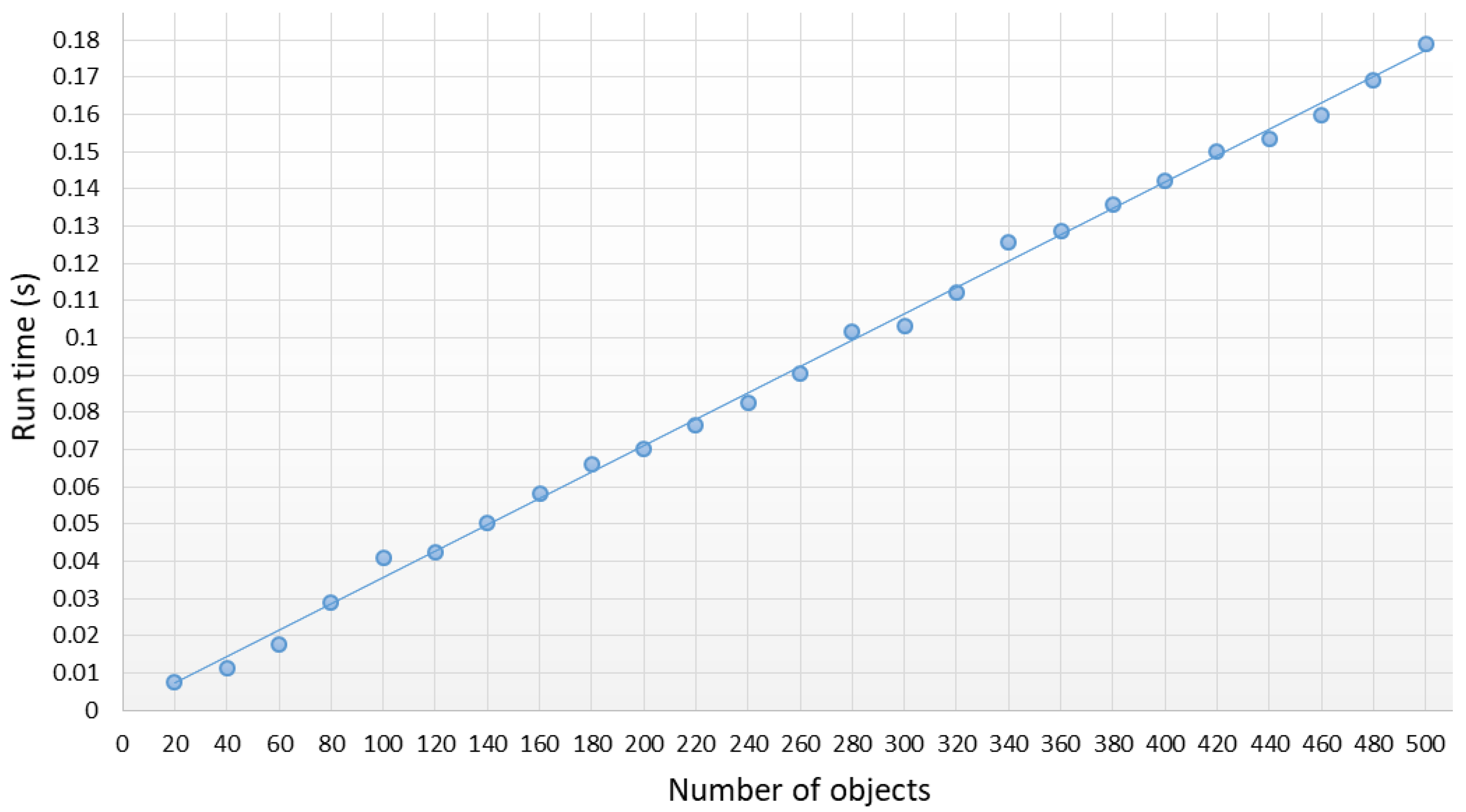
Based on the generated initial data, we calculate the area $\mathsf{\mu }\left(\mathsf{\Omega }(\mathbf{g})\right)$ of a complex object $\mathsf{\Omega }(\mathbf{g})$, the structure of which is determined by Formula (3). The Shapely library was used to build $\mathsf{\Omega }(\mathbf{g})$ and calculate its area.

Figure 1 shows the dependence of the average time of calculating the area $\mathsf{\mu }\left(\mathsf{\Omega }(\mathbf{g})\right)$ on the number of ellipses ${\mathrm{S}}_{\mathrm{i}},\hspace{0.17em}\mathrm{i}\in {\mathbf{J}}_{\mathrm{n}}^{}$ covering the rectangle ${\mathrm{S}}_0$. Averaging was performed on 20 independent tests.

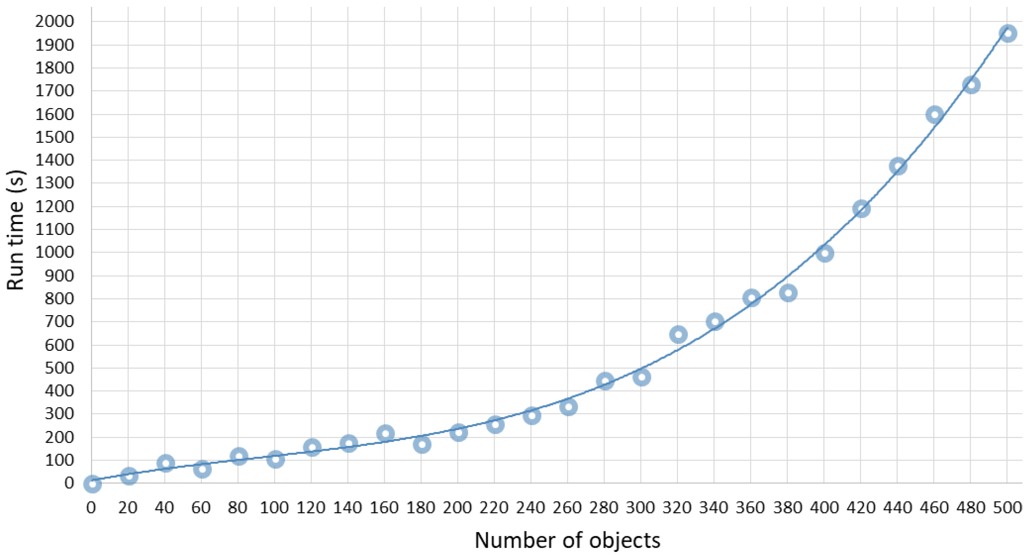
The next experiment is to study the time of obtaining a local solution to problem (9). For local optimization, the SciPy package was chosen, which implements the BFGS method [37] using first order differences. The gradient was estimated by Formula (14). For each of the previously formed test tasks, the placement parameters ${\mathbf{p}}^{\mathrm{i}}=({\mathrm{x}}_{\mathrm{i}},{\mathrm{y}}_{\mathrm{i}},{\mathsf{\theta }}_{\mathrm{i}}),\hspace{0.33em}\mathrm{i}\in {\mathbf{J}}_{\mathrm{n}}^{}$ randomly generated at the previous stage during the formation of a complex object were chosen as a starting point.

Figure 2 shows the dependence of the average time to obtain a local solution on the number of ellipses. Averaging was carried out over 10 independent tests. Formula (14) was used instead of (11) to estimate first-order differences when calculating the gradient of function ${\mathsf{\omega }}_{\mathsf{\Omega }}(\mathbf{g})$.

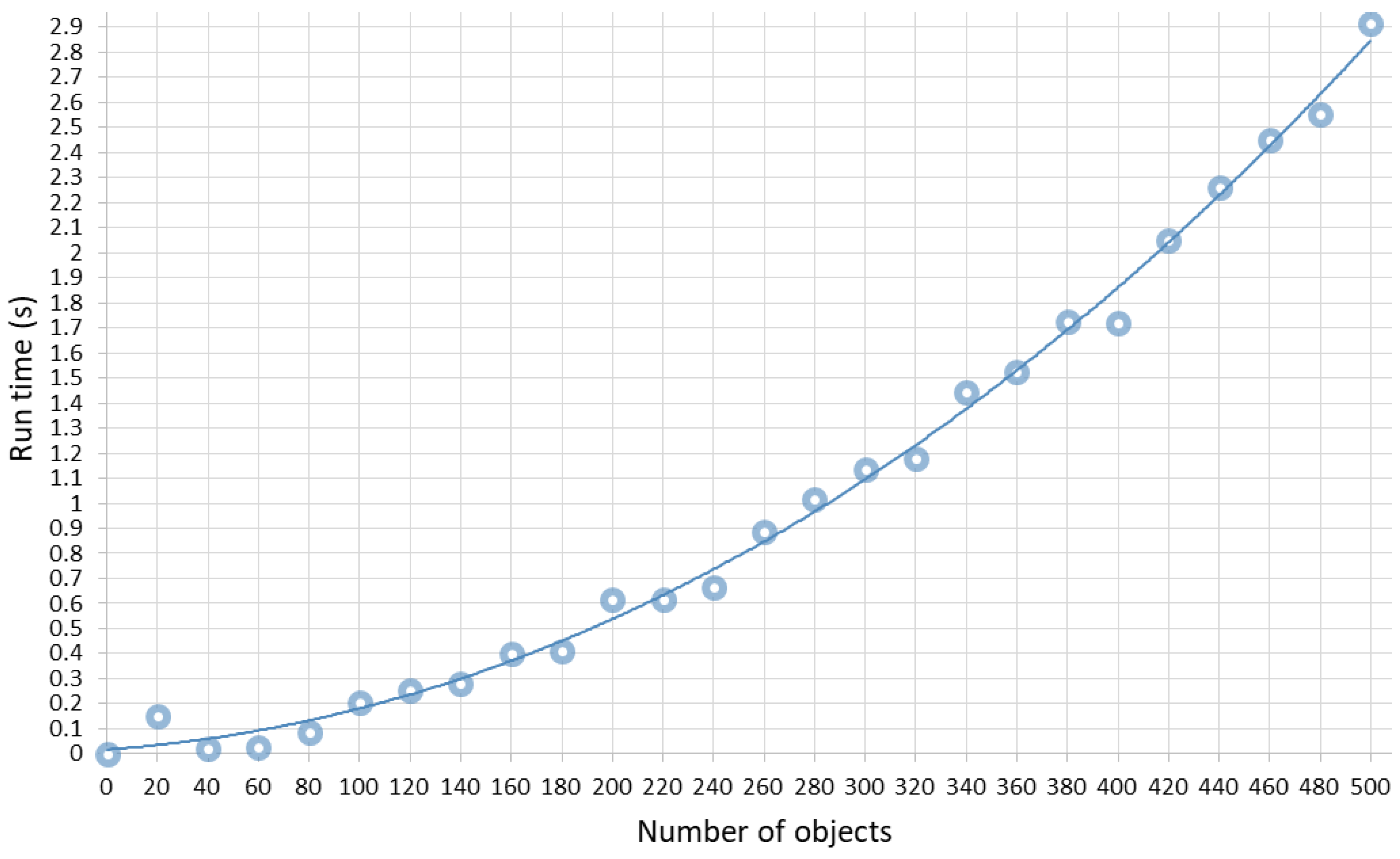
To substantiate this approach, we studied the dependence of the formation time of the matrix of pairwise intersections (12) on its dimension. Figure 3 illustrates such dependence.

The data shown in Figure 3 allows us to estimate the average time for calculating the area of intersection of two objects. To do this, you need to sum all the elements of the matrix and divide by their number. Analyzing the obtained results, it can be argued that the estimation of the gradient using the matrix $\mathrm{M}$ requires much less time than by calculating the function $\mathsf{\mu }\left(\mathsf{\Omega }(\mathbf{g})\right)$. Indeed, with n=100, the time for calculating the increment of a function by Formula (11) is $0.04\times 2=0.08 \mathrm{s}$, and the average time for the formation of the upper triangular matrix $\mathrm{M}$ is 0.2 s. Therefore, to calculate the area of intersection of each two objects, $0.2\times 2/(100\times 101)=0.000039604 \mathrm{s}$ is required. Since to estimate ${\Delta }_{\mathrm{k}}^{\mathrm{i}}{\mathsf{\omega }}_{\mathsf{\Omega }}(\hat{\mathbf{g}})$ using Formula (14) it is necessary to sum the areas of pairwise intersections of one object with the other 100, this will require $0.0039604 \mathrm{s}$. You can see the same when n = 500. The function ${\mathsf{\omega }}_{\mathsf{\Omega }}(\hat{\mathbf{g}})$ calculation time is 0.18 s and the matrix $\mathrm{M}$ formation time is 2.7 s. The function increment ${\Delta }_{\mathrm{k}}^{\mathrm{i}}{\mathsf{\omega }}_{\mathsf{\Omega }}(\hat{\mathrm{g}})$ according to Formula (14) will be calculated approximately in $2.7\times 2/501=0.01078 \mathrm{s}$.

Let us apply the described approach to solving the following test problems of maximum coverage. Let the covering objects be ellipses with semi-axis $({\mathrm{a}}_{\mathrm{i}},{\mathrm{b}}_{\mathrm{i}}),\hspace{0.17em}\mathrm{i}\in {\mathbf{J}}_{\mathrm{n}}^{},\mathrm{n}=100$ listed in

Table A1. Metrical parameters of ellipses.

i	ai	bi	i	ai	bi	i	ai	bi	i	ai	bi
1	1.5	1.3	26	1.5	1.5	51	4.5	2.5	76	4.5	2.0
2	1.9	1.4	27	1.9	1.8	52	4.9	2.8	77	4.9	2.2
3	2.4	2.0	28	2.4	1.2	53	5.4	2.2	78	5.4	3.2
4	2.9	2.0	29	2.9	1.5	54	5.9	3.5	79	5.9	3.5
5	3.3	1,7	30	3.3	1.3	55	6.3	2.3	80	6.3	3.3
6	3.8	1.9	31	3.8	2.9	56	6.8	3.5	81	6.8	2.8
7	4.5	2.0	32	4.5	3.0	57	7.5	3.3	82	7.5	4.0
8	4.9	2.5	33	4.9	2.5	58	7.9	4.5	83	7.9	3.4
9	5.0	2.4	34	5.0	3.4	59	8.0	3.4	84	8.0	4.4
10	5.4	2.3	35	5.4	2.3	60	8.4	2.7	85	8.4	4.1
11	5.9	3.1	36	5.9	2.1	61	8.9	4.1	86	8.9	3.3
12	6.1	3.0	37	6.1	1.5	62	9.1	3.5	87	9.1	4.6
13	6.4	2.8	38	6.4	2.8	63	9.4	3.8	88	9.4	3.2
14	6.6	3.5	39	6.6	2.9	64	9.6	4.5	89	9.6	3.5
15	7.0	3.0	40	7.0	4.0	65	10.1	4.0	90	10.1	5.2
16	7.1	3.5	41	7.1	2.5	66	10.4	2.5	91	10.4	4.5
17	7.3	3.3	42	7.3	3.7	67	10.7	3.7	92	10.7	5.7
18	7.6	2.9	43	7.6	3.9	68	11.0	4.9	93	11.0	3.9
19	7.9	3.5	44	7.9	2.5	69	11.4	3.5	94	11.4	4.5
20	8.1	4.0	45	8.1	3.0	70	11.8	5.0	95	11.8	4.0
21	8.3	5.0	46	8.3	4.0	71	12.1	5.0	96	12.1	4.0
22	8.5	4.5	47	8,5	3.5	72	12.5	4.5	97	12.5	3.5
23	8.8	5.5	48	8.8	4.5	72	13.1	5.5	98	13.1	4.5
24	8.8	3.1	49	8.8	4.1	74	13.6	6.1	99	13.6	4.1
25	9.0	5.9	50	9.0	3.9	75	14.0	4.0	100	14.0	3.9

(Appendix A).

The problems of unconditional local optimization (9) for n = 30, 50, 75, 100 was solved. Squares with sides 30, 40, 70, and 70 for n = 30, 50, 70, and 100, respectively, were chosen as the coverage domain. BFGS method using first-order differences was used. The gradients was estimated by Formula (14). The starting point for BFGS method was chosen by random generation of ellipse placement parameters by analogy with the experiments described earlier.

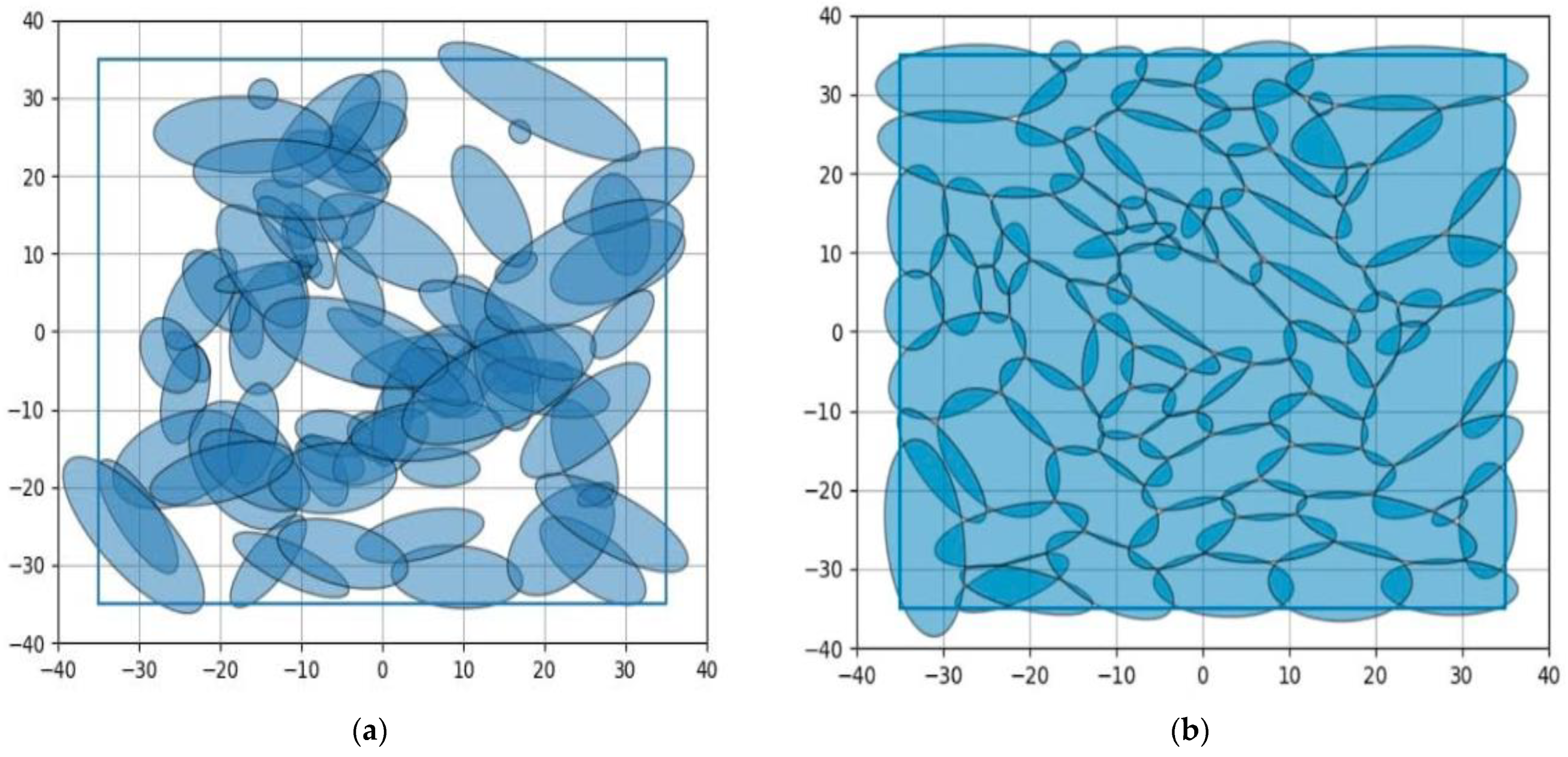
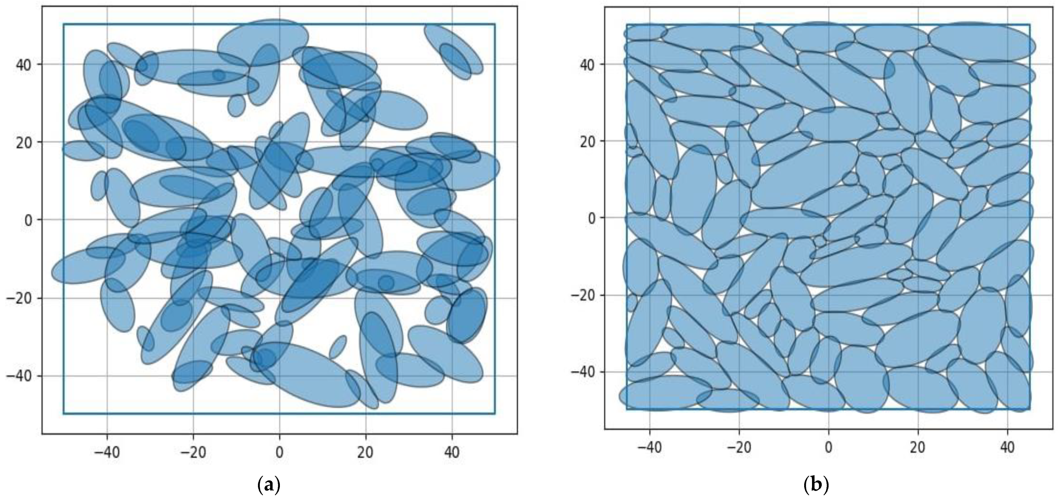
Figure 4, Figure 5, Figure 6 and Figure 7 show the initial location of the ellipses in the coverage domain and the placement obtained as a result of local optimization for n = 30, 50, 75, and 100. The run times to solve the problems are 22 s, 51 s, 79 s, and 103 s, respectively.

Let us pay special attention to the test problems when n = 50 and n = 75. At n = 50, due to the large size of the coverage domain, such an placement of ellipses was obtained in which they do not intersect and are located inside the area. This is a global solution to problem (9), which corresponds to the so-called packing configuration [28,29]. For n = 75, each point of the coverage domain belongs to at least one of the covering objects. This is also a global solution to problem (9), and the resulting location defines the so-called covering configuration [28,29].

5. Discussion

The maximum coverage location problem is related to the determination of the placement of objects in order to cover as much as possible of the domain served by them. Such problems are formulated in discrete, continuous, and mixed statements, taking into account their geometric features.

The choice of one or another model depends on the restrictions on the location of objects and the properties of the service area. The classical discrete setting assumes that both object locations and service areas are isolated points. The weakening of the discreteness conditions leads to continuous and mixed formulations.

This article is perhaps one of the first to raise questions of formalization of completely continuous MCLP. In this case, both the locations and the service area are continual and suggest the possibility of their continuous transformation.

Of course, by discretizing the coverage area, for example, by grid methods, one can reduce continuous problems to discrete formulations. However, in this case, we will rather talk about the method of solution, and not about an adequate mathematical statement of the problem.

The geometric features of the continuous MCLP are related to both the shape of the covering objects and the service area. In turn, the problems go beyond the class of classical coverage problems, in which each point of the domain must belong to at least one of the covering objects. Therefore, continuous MCLP require the construction of special mathematical models and optimization methods that take into account their specifics.

The continuous MCLP model as a non-linear unconstrained optimization problem opens up prospects for using both modern effective methods for solving them and existing software in the form of powerful packages for various computer platforms.

The conducted studies allowed us to approach the analysis of the mathematical model of the problem from a unified standpoint. On the one hand, knowing the equations of general position of geometric objects ${\mathrm{S}}_{\mathrm{i}}({\mathbf{g}}^{\mathrm{i}}),\mathrm{i}\in {\mathbf{J}}_{\mathrm{n}}^0$, used in the formation of a complex object $\mathsf{\Omega }(\mathbf{g})$, one can write down the equation of its boundary. Therefore, formally we will find the analytical form of the function ${\mathsf{\omega }}_{\mathsf{\Omega }}(\mathbf{g})=\mathsf{\mu }\left(\mathsf{\Omega }(\mathbf{g})\right)$ depending on the generalized variables $\mathbf{g}$. As a result, we will obtain an expression in the form of an integral depending on a vector parameter, for the calculation of which we will have to use numerical methods. This approach is very time consuming and is associated with the consideration of various options for the acceptable location of objects.

The approach proposed in the paper is devoid of these shortcomings. All the difficulties associated with the analytical specification of the function ${\mathsf{\omega }}_{\mathsf{\Omega }}(\mathrm{g})$ are overcome by using computer geometry packages that work great with geometric objects of complex spatial shape. As a result, it takes milliseconds to calculate the function value ${\mathsf{\omega }}_{\mathsf{\Omega }}(\hat{\mathbf{g}})$ for the fixed $\hat{\mathbf{g}}$, which is confirmed by the experiments described in the Section 4. This justifies the possibility of using metaheuristic methods of global optimization [38,39]. The efficiency of methods increases significantly if it is possible to use local optimization methods. The simplest is the multistart scheme for generation $\mathsf{\Omega }(\hat{\mathbf{g}})$ with subsequent local optimization of the function ${\mathsf{\omega }}_{\mathsf{\Omega }}(\mathbf{g})$, choosing $\hat{\mathbf{g}}$ as the starting point. With limited time, the data illustrated in Figure 2 allows an estimate of the number of iterations in the multistart method. If temporary resources allow, hybrid methods can be proposed, where local optimization is applied after improvements have been received.

The geometrical features of the continuous MCLP model have made it possible to significantly increase the efficiency of local optimization methods using first order differences. This is confirmed by the data shown in Figure 3.

In general, the proposed approach opens up prospects for the development of new methods for solving both packing and covering problems. Indeed, in the course of the experiments, we obtained such locations of objects that corresponded to the packing configuration (Figure 5b) and covering configuration (Figure 6b). Thus, the introduction of additional conditions on the value of the function will allow us to propose new mathematical models for classical packing and covering problems and methods for their solution. In particular, the constraint

$${\mathsf{\omega }}_{\mathsf{\Omega }}(\mathbf{g})={\displaystyle \sum _{\mathrm{i}=1}^{\mathrm{n}}\mathsf{\mu }({\mathrm{S}}_{\mathrm{i}})},$$

(17)

is the condition for both non-intersection of objects ${\mathrm{S}}_{\mathrm{i}}({\mathbf{g}}^{\mathrm{i}})$, $\mathrm{i}\in {\mathbf{J}}_{\mathrm{n}}^{}$, and their inclusion inside the container ${\mathrm{S}}_0$.

The constraint

$${\mathsf{\omega }}_{\mathsf{\Omega }}(\mathbf{g})=\mathsf{\mu }({\mathrm{S}}_0),$$

(18)

is a condition for covering the domain ${\mathrm{S}}_0$ by a family of geometric objects ${\mathrm{S}}_{\mathrm{i}}({\mathbf{g}}^{\mathrm{i}}),\mathrm{i}\in {\mathbf{J}}_{\mathrm{n}}^0$.

Note that the choice of the BFGS method for local optimization was based on high user ratings. Of course, further studies of continuous MCLP require a comparative analysis of modern optimization methods, in particular [40]. Potential decision improvements can be obtained by using a novel optimization scheme, such as deep learned recurrent type-3 fuzzy system [41].

Another promising direction is the study of optimization problems of packing and coverage in domains with variable metric parameters. The results described in this article are directly related to this problem as well.