
A Prospective Method for Generating COVID-19 Dynamics

 ,
,  , , , ,
  and
and
Abstract
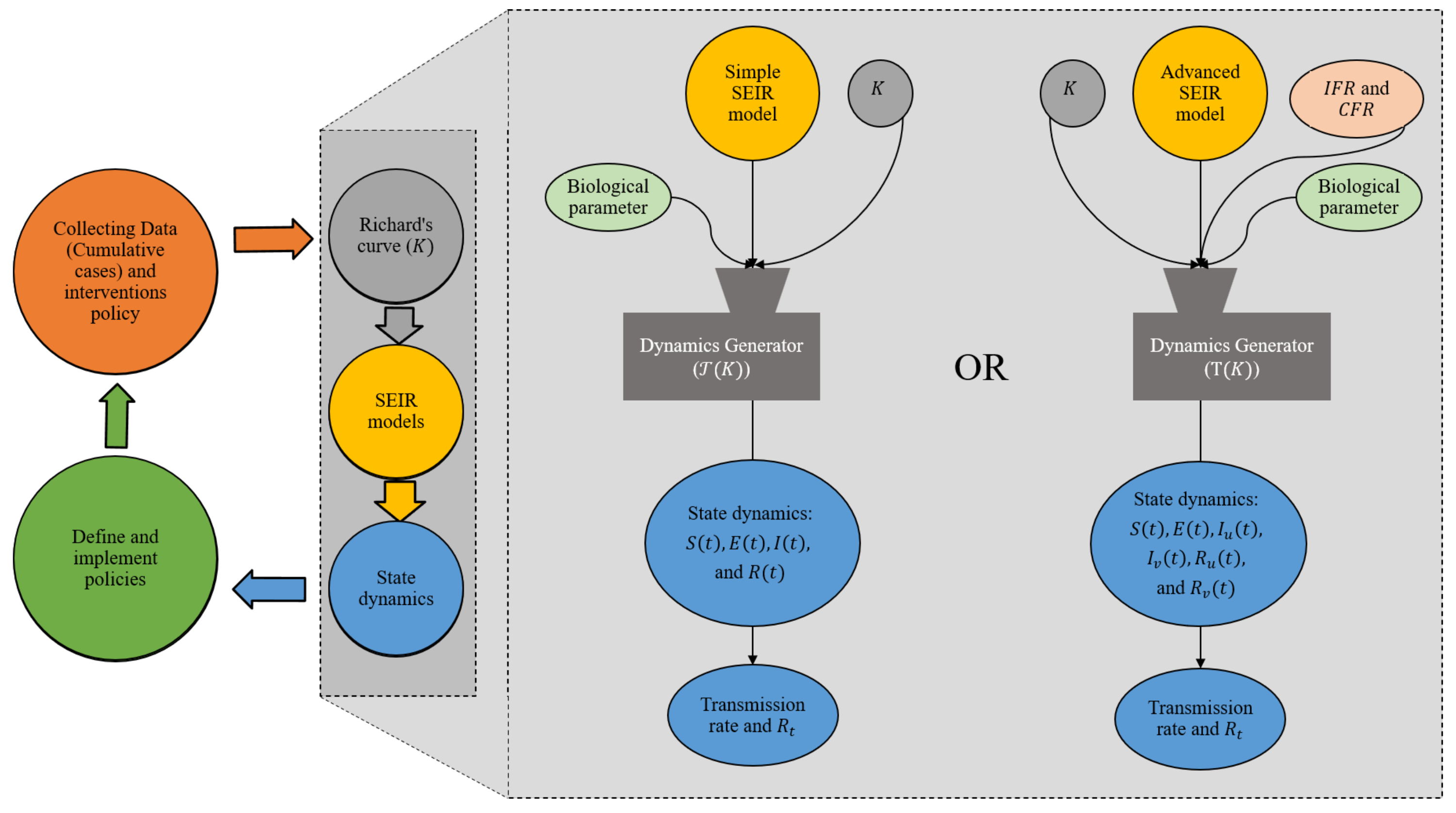
:1. Introduction
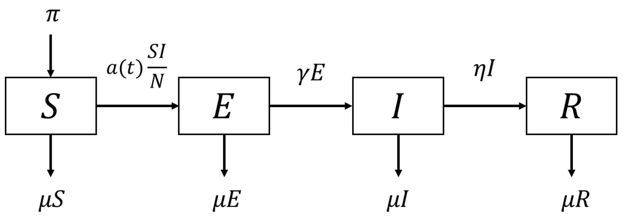
2. Generating Operator in a Simple SEIR Model
2.1. Model Formulation
2.2. Cumulative Case Data for Constructing the Generating Operator
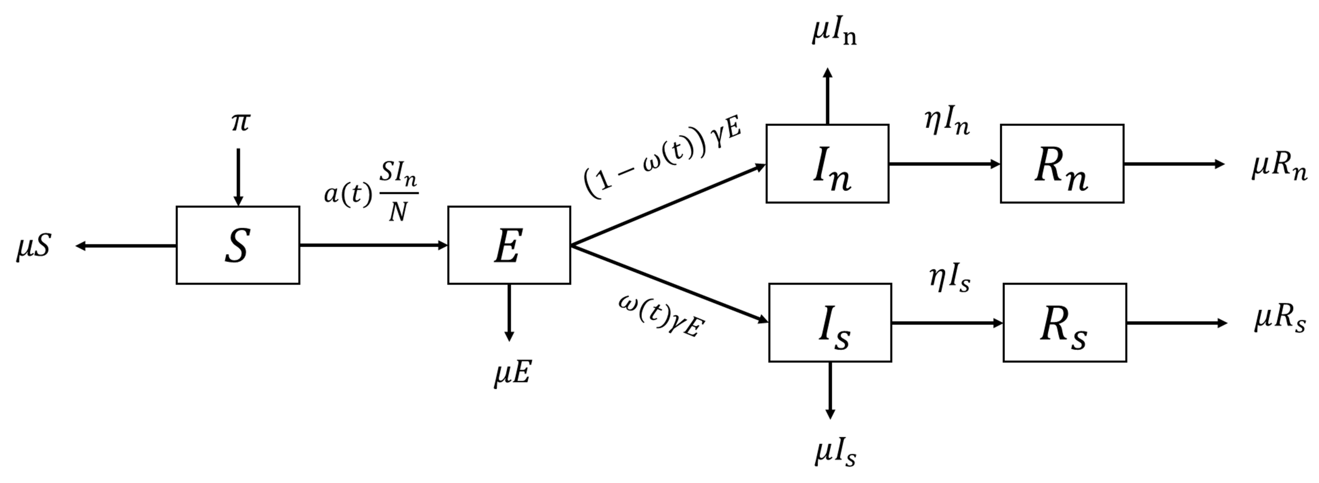
3. Generalized SEIR for Second Wave Transmission of COVID-19
3.1. Model Construction
3.2. Estimation of
4. Numerical Simulations
4.1. Simple SEIR Model
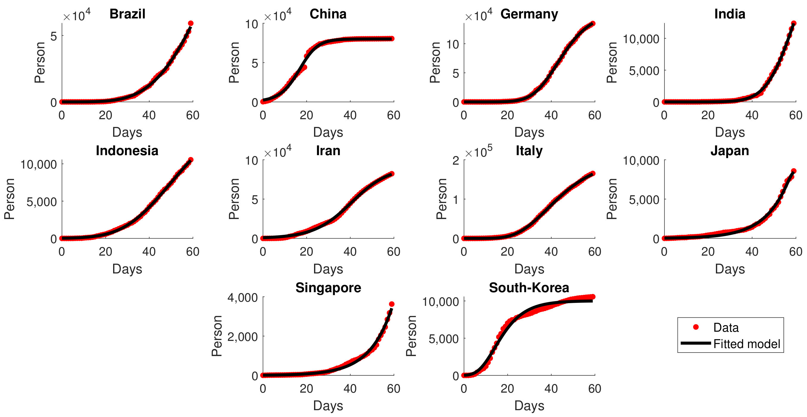
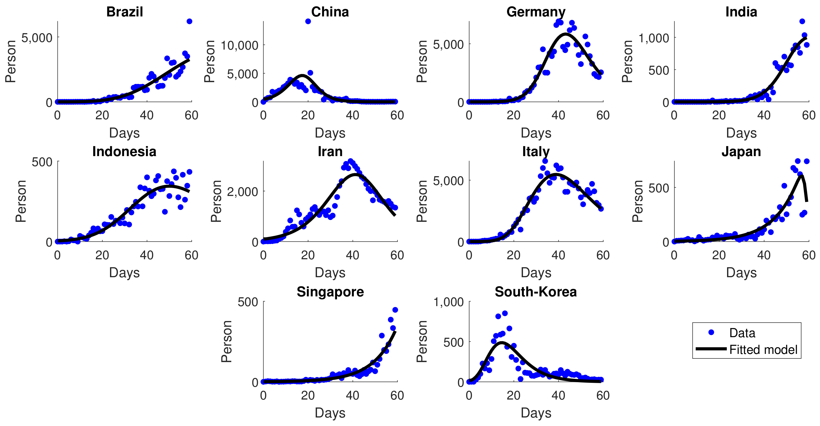
4.1.1. Fitted Cumulative Data
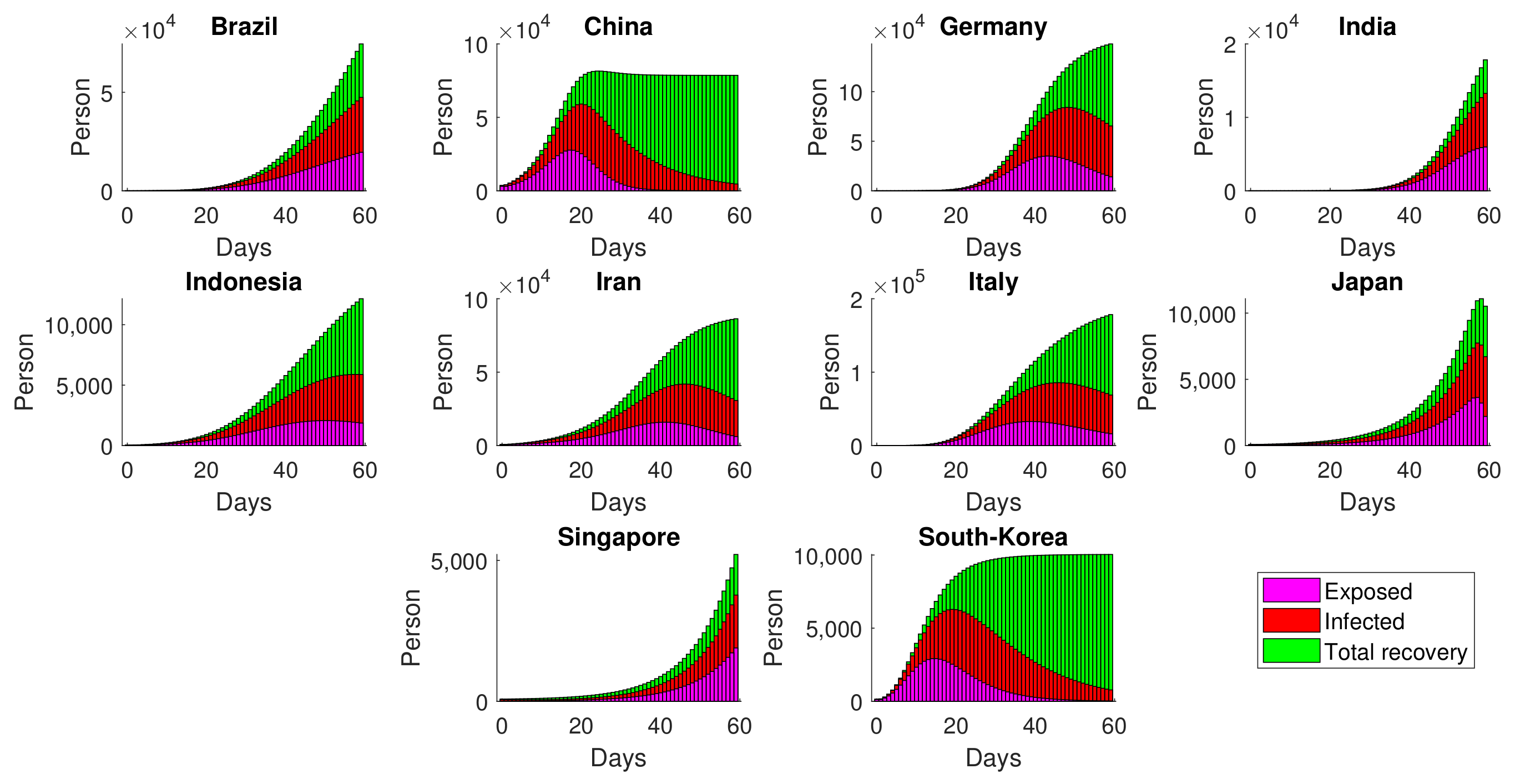
4.1.2. Simulation of SEIR Dynamics
4.1.3. Dynamics of the Effective Reproduction Number
4.2. Generalized SEIR Model
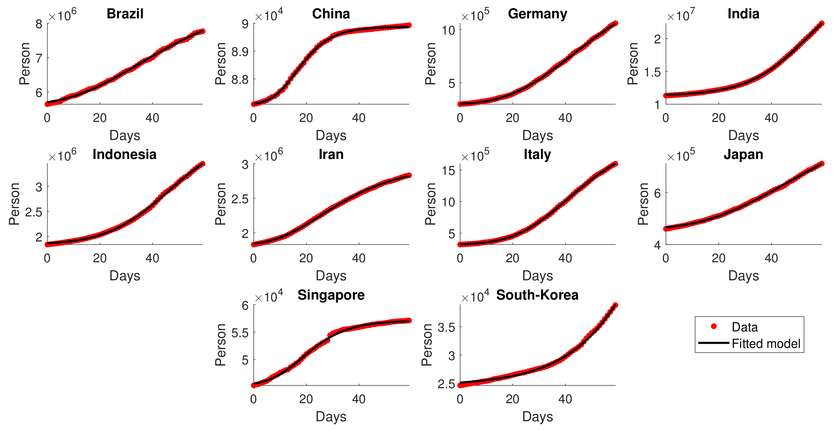
4.2.1. Fitted Cumulative Data
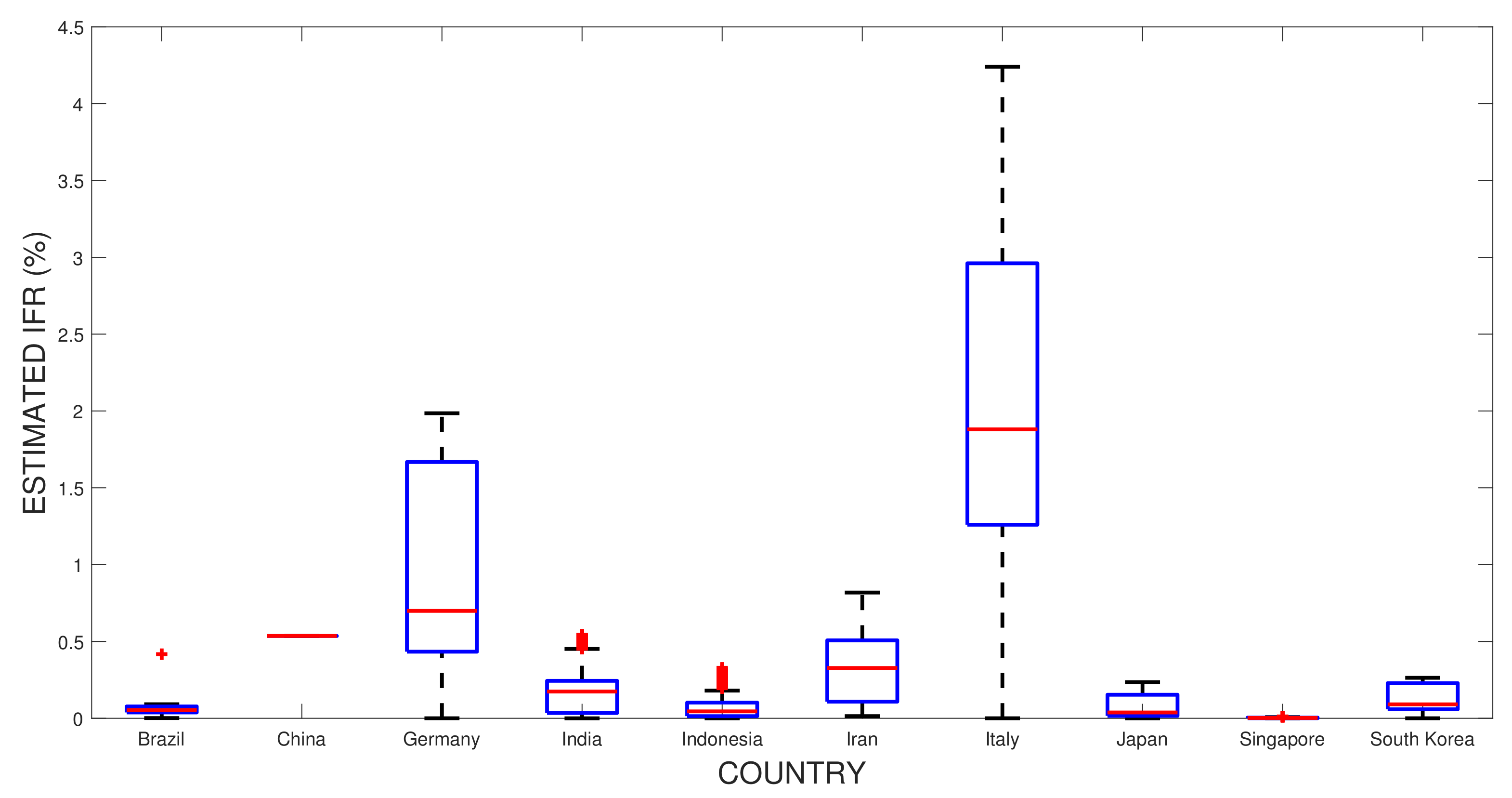
4.2.2. Estimated
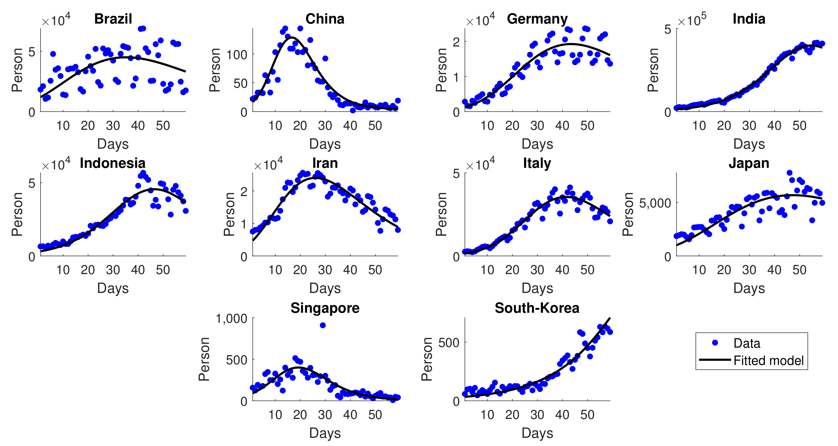
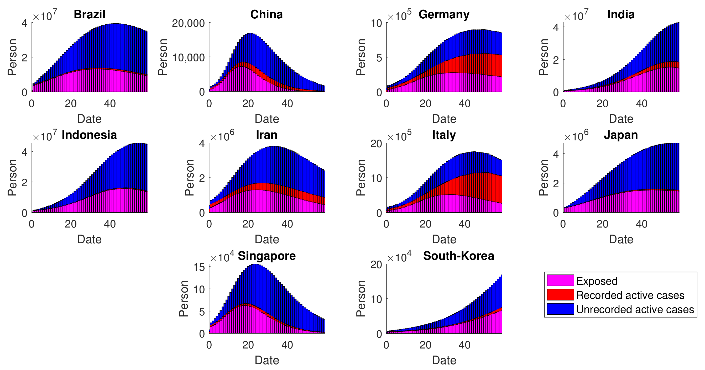
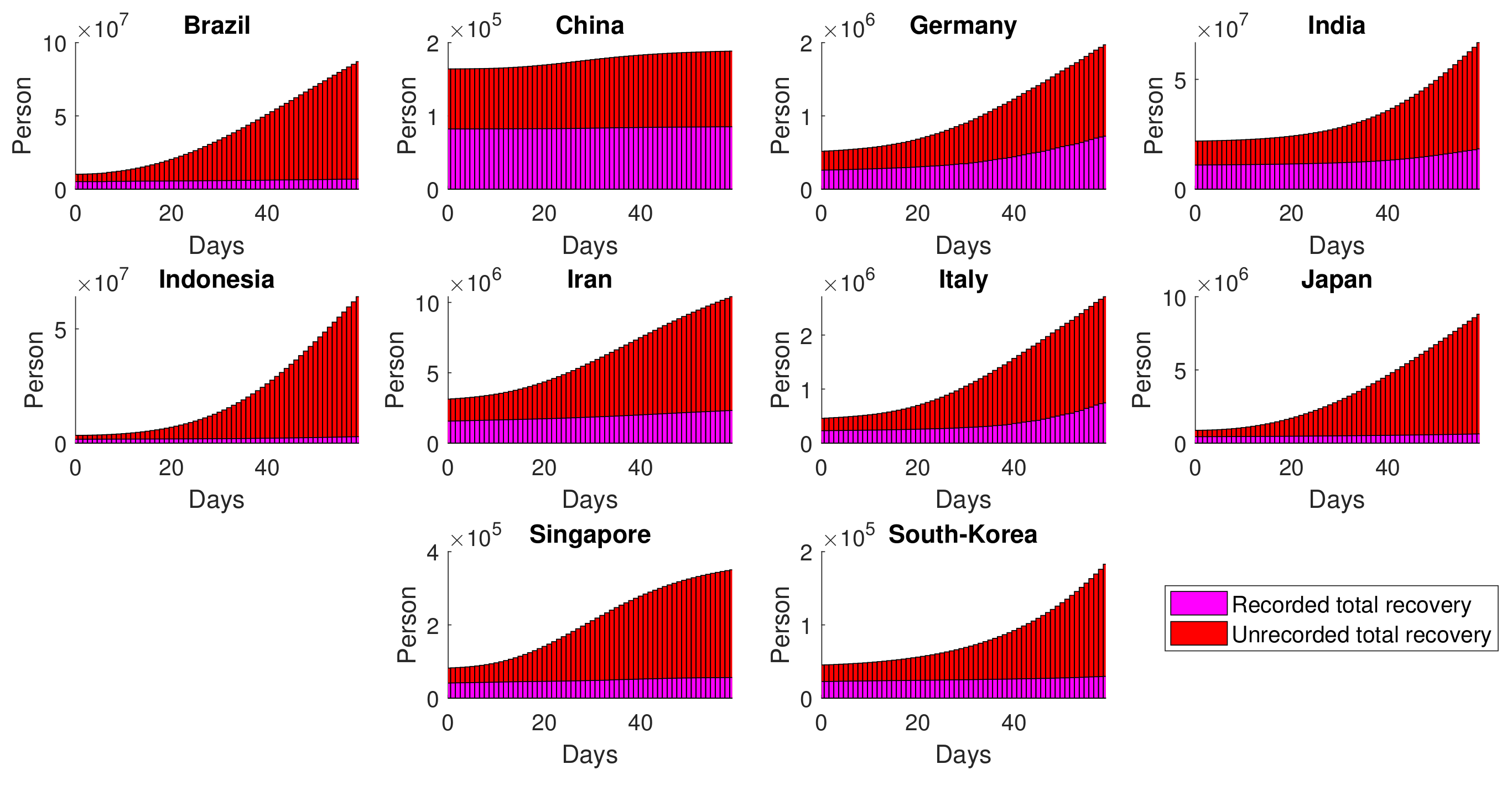
4.2.3. Dynamics of the Generalized SEIR Model
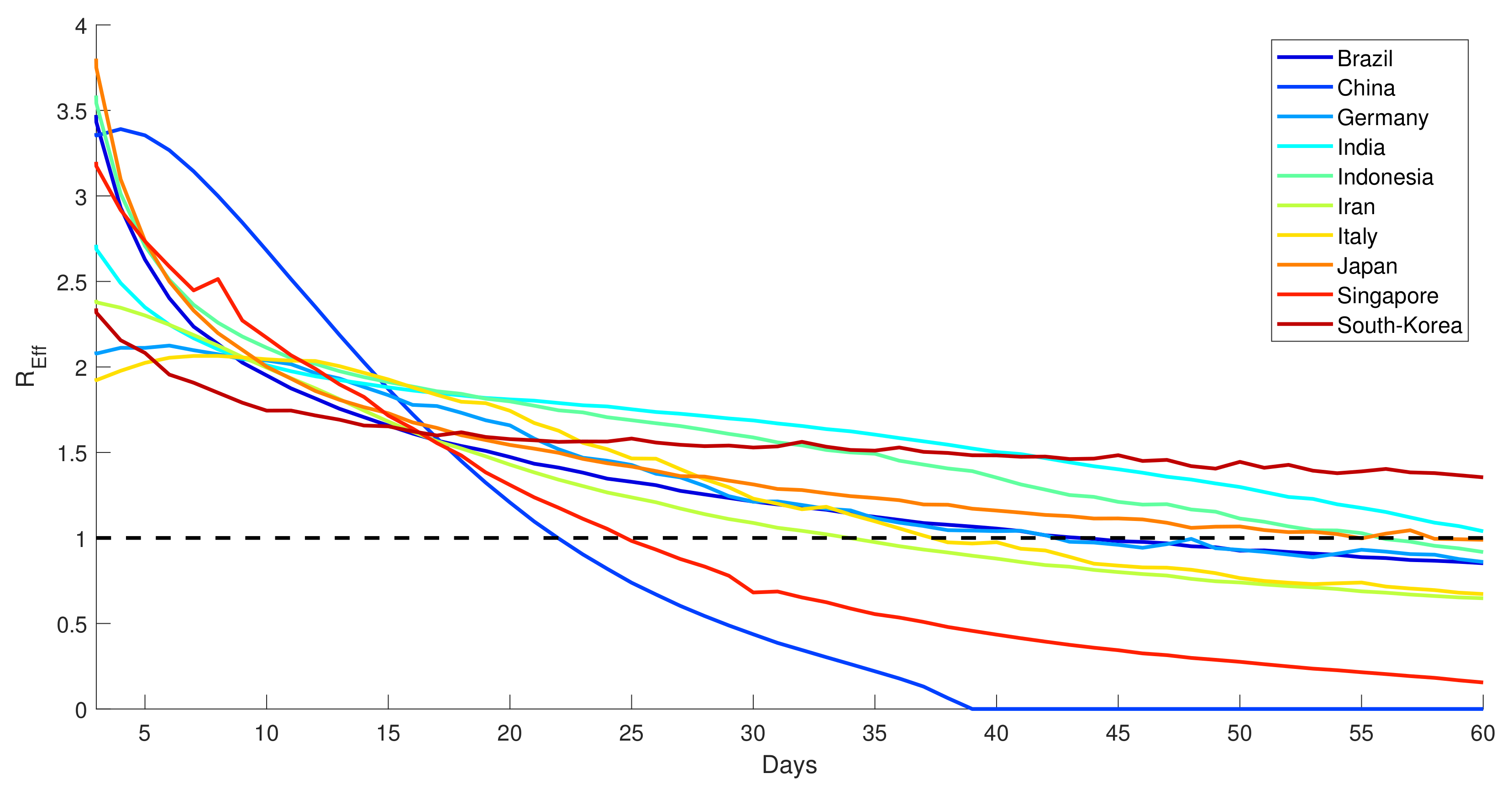
4.3. More about the Effective Reproduction Number
5. Conclusions
Author Contributions
Funding
Institutional Review Board Statement
Informed Consent Statement
Data Availability Statement
Conflicts of Interest
References
- Novel Coronavirus (2019-nCoV)—Situation Report 1. Available online: https://www.who.int/docs/default-source/coronaviruse/situation-reports/20200121-sitrep-1-2019-ncov.pdf (accessed on 5 April 2021).
- Andersen, K.G.; Rambaut, A.; Lipkin, W.I.; Holmes, E.C.; Garry, R.F. The proximal origin of SARS-CoV-2. Nat. Med. 2020, 26, 450–452. [Google Scholar] [CrossRef] [Green Version]
- Huang, C.; Wang, Y.; Li, X.; Ren, L.; Zhao, J.; Hu, Y.; Zhang, L.; Fan, G.; Xu, J.; Gu, X.; et al. Clinical features of patients infected with 2019 novel coronavirus in Wuhan, China. Lancet 2020, 395, 497–506. [Google Scholar] [CrossRef] [Green Version]
- Singhal, T. A review of coronavirus disease-2019 (COVID-19). Indian J. Pediatr. 2020, 87, 281–286. [Google Scholar] [CrossRef] [Green Version]
- Zhang, Y.; You, C.; Cai, Z.; Sun, J.; Hu, W.; Zhou, X.H. Prediction of the COVID-19 outbreak in China based on a new stochastic dynamic model. Sci. Rep. 2020, 10, 21522. [Google Scholar] [CrossRef]
- Bertozzi, A.; Franco, E.; Mohler, G.; Short, M.; Sledge, D. The challenges of modeling and forecasting the spread of COVID-19. Proc. Natl. Acad. Sci. USA 2020, 117, 16732–26738. [Google Scholar] [CrossRef]
- Nuraini, N.; Khairudin, K.; Apri, M. Modeling simulation of COVID-19 in Indonesia based on early endemic data. Commun. Biomath. Sci. 2020, 3, 1–8. [Google Scholar] [CrossRef]
- Sucahya, P.K. Barriers to COVID-19 RT-PCR Testing in Indonesia: A Health Policy Perspective. J. Indones. Health Policy Adm. 2020, 5, 36–42. [Google Scholar] [CrossRef]
- Indonesia’s Lab Problems Persist, Testing Rate Remains Below 1%. Available online: https://www.thejakartapost.com/news/2020/10/22/ri-lab-problems-persist-testing-rate-remains-below-1.html (accessed on 2 May 2021).
- Yang, Z.; Zeng, Z.; Wang, K.; Wong, S.S.; Liang, W.; Zanin, M.; Liu, P.; Cao, X.; Gao, Z.; Mai, Z.; et al. Modified SEIR and AI prediction of the epidemics trend of COVID-19 in China under public health interventions. J. Thorac. Dis. 2020, 12, 165. [Google Scholar] [CrossRef]
- Ross, R. An application of the theory of probabilities to the study of a priori pathometry—Part I. Proc. R. Soc. Lond. Ser. A Contain. Pap. A Math. Phys. Character 1916, 92, 204–230. [Google Scholar]
- Susanto, H.; Tjahjono, V.; Hasan, A.; Kasim, M.; Nuraini, N.; Putri, E.; Kusdiantara, R.; Kurniawan, H. How many can you infect? Simple (and naive) methods of estimating the reproduction number. Commun. Biomath. Sci. 2020, 3, 28–36. [Google Scholar] [CrossRef]
- Soewono, E. On the analysis of COVID-19 transmission in Wuhan, Diamond Princess and Jakarta-cluster. Commun. Biomath. Sci. 2020, 3, 9–18. [Google Scholar] [CrossRef]
- Azque-Herrerias, F.; Munuzuri-Perez, V.; Galla, T. Stirring does not make populations well mixed. Sci. Rep. 2018, 8, 4068. [Google Scholar] [CrossRef] [Green Version]
- World Population by Countries. Available online: https://www.worldometers.info/world-population/#density (accessed on 9 July 2021).
- Human Life Expectancy. Available online: https://www.worldometers.info/world-population/indonesia-population/ (accessed on 7 March 2021).
- Lauer, S.A.; Grantz, K.H.; Bi, Q.; Jones, F.K.; Zheng, Q.; Meredith, H.R.; Azman, A.S.; Reich, N.G.; Lessler, J. The incubation period of coronavirus disease 2019 (COVID-19) from publicly reported confirmed cases: Estimation and application. Ann. Intern. Med. 2020, 172, 577–582. [Google Scholar] [CrossRef] [Green Version]
- Transmission of SARS-CoV-2: Implications for Infection Prevention Precautions. Available online: https://www.who.int/news-room/commentaries/detail/transmission-of-sars-cov-2-implications-for-infection-prevention-precautions (accessed on 6 April 2021).
- Diekmann, O.; Heesterbeek, J.; Roberts, M.G. The construction of next-generation matrices for compartmental epidemic models. J. R. Soc. Interface 2010, 7, 873–885. [Google Scholar] [CrossRef] [Green Version]
- Ahamad, M.G.; Tanin, F.; Talukder, B.; Ahmed, M.U. Officially Confirmed COVID-19 and Unreported COVID-19—Like Illness Death Counts: An Assessment of Reporting Discrepancy in Bangladesh. Am. J. Trop. Med. Hyg. 2021, 104, 546. [Google Scholar] [CrossRef]
- Vasudevan, V.; Gnanasekaran, A.; Sankar, V.; Vasudevan, S.A.; Zou, J. Disparity in the quality of COVID-19 data reporting across India. BMC Public Health 2021, 21, 1211. [Google Scholar] [CrossRef]
- Woolf, S.H.; Chapman, D.A.; Sabo, R.T.; Weinberger, D.M.; Hill, L. Excess deaths from COVID-19 and other causes, March-April 2020. J. Am. Med. Assoc. 2020, 324, 510–513. [Google Scholar] [CrossRef]
- Ioannidis, J.P.; Cripps, S.; Tanner, M.A. Forecasting for COVID-19 has failed. Int. J. Forecast. 2020, 38, 423–438. [Google Scholar] [CrossRef]
- Richards, F. A flexible growth function for empirical use. J. Exp. Bot. 1959, 10, 290–301. [Google Scholar] [CrossRef]
- Lei, Y.; Zhang, S. Features and partial derivatives of Bertalanffy-Richards growth model in forestry. Nonlinear Anal. Model. Control 2004, 9, 65–73. [Google Scholar] [CrossRef]
- Lee, S.Y.; Lei, B.; Mallick, B. Estimation of COVID-19 spread curves integrating global data and borrowing information. PLoS ONE 2020, 15, e0236860. [Google Scholar] [CrossRef]
- Germany Is Poised to Tighten Lockdown as COVID-19 Cases Surge Again. Available online: https://www.wsj.com/livecoverage/covid-2021-03-22/card/h7nDLKXUj1H0yZJsgeoI (accessed on 2 August 2021).
- S. Korea Sees Rise in Cases after Relaxing Social Distancing Rules. Available online: http://www.koreaherald.com/view.php?ud=20201102000137 (accessed on 4 July 2021).
- ‘The Perfect Storm’: Lax Social Distancing Fuelled a Coronavirus Variant’s Brazilian Surge. Available online: https://www.nature.com/articles/d41586-021-01480-3 (accessed on 4 July 2021).
- Fiore, V.G.; DeFelice, N.; Glicksberg, B.S.; Perl, O.; Shuster, A.; Kulkarni, K.; O’Brien, M.; Pisauro, M.A.; Chung, D.; Gu, X. Containment of COVID-19: Simulating the impact of different policies and testing capacities for contact tracing, testing, and isolation. PLoS ONE 2021, 16, e0247614. [Google Scholar] [CrossRef]
- Daily COVID-19 Tests. Available online: https://ourworldindata.org/grapher/daily-COVID-19-tests-smoothed-7-day (accessed on 7 September 2021).
- Case Fatality Rate. Available online: https://www.britannica.com/science/case-fatality-rate (accessed on 23 August 2021).
- Streeck, H.; Schulte, B.; Kümmerer, B.M.; Richter, E.; Höller, T.; Fuhrmann, C.; Bartok, E.; Dolscheid-Pommerich, R.; Berger, M.; Wessendorf, L.; et al. Infection fatality rate of SARS-CoV2 in a super-spreading event in Germany. Nat. Commun. 2020, 11, 5829. [Google Scholar] [CrossRef]
- Teppone, M. One Year of COVID-19 Pandemic: Case Fatality Ratio and Infection Fatality Ratio. A Systematic Analysis of 219 Countries and Territories. Preprints 2021, 1–13. [Google Scholar] [CrossRef]
- Ioannidis, J.P. Infection fatality rate of COVID-19 inferred from seroprevalence data. Bull. World Health Organ. 2021, 99, 19. [Google Scholar] [CrossRef]
- Mallapaty, S. How deadly is the coronavirus? Scientists are close to an answer. Nature 2020, 582, 467–469. [Google Scholar] [CrossRef]
- Reported Cases and Deaths by Country or Territory. Available online: https://www.worldometers.info/coronavirus/#countries (accessed on 21 March 2021).
- Kraemer, M.U.; Yang, C.H.; Gutierrez, B.; Wu, C.H.; Klein, B.; Pigott, D.M.; Open COVID-19 Data Working Group; du Plessis, L.; Faria, N.R.; Li, R.; et al. The effect of human mobility and control measures on the COVID-19 epidemic in China. Science 2020, 368, 493–497. [Google Scholar] [CrossRef] [Green Version]
- Choi, S.; Ki, M. Estimating the reproductive number and the outbreak size of COVID-19 in Korea. Epidemiol. Health 2020, 42, e2020011. [Google Scholar] [CrossRef]
- Chowell, G. Fitting dynamic models to epidemic outbreaks with quantified uncertainty: A primer for parameter uncertainty, identifiability, and forecasts. Infect. Dis. Model. 2017, 2, 379–398. [Google Scholar] [CrossRef]
- China Reports Most New COVID-19 Cases Since January amid Delta Surge. Available online: https://www.reuters.com/world/china/china-reports-96-new-coronavirus-cases-aug-3-vs-90-day-ago-2021-08-04/ (accessed on 5 August 2021).
- Coronavirus Digest: Germany Cases Surge to New Record. Available online: https://www.dw.com/en/coronavirus-digest-germany-cases-surge-to-new-record/a-55292392 (accessed on 5 August 2021).
- Lai, A.; Bergna, A.; Menzo, S.; Zehender, G.; Caucci, S.; Ghisetti, V.; Rizzo, F.; Maggi, F.; Cerutti, F.; Giurato, G.; et al. Circulating SARS-CoV-2 Variants in Italy, October 2020–March 2021. Virol. J. 2021, 18, 168. [Google Scholar] [CrossRef]
- Visaria, A.; Dharamdasani, T. The complex causes of India’s 2021 COVID-19 surge. Lancet 2021, 397, 2464. [Google Scholar] [CrossRef]
- Luo, G.; Zhang, X.; Zheng, H.; He, D. Infection fatality ratio and case fatality ratio of COVID-19. Int. J. Infect. Dis. 2021, 113, 43–46. [Google Scholar] [CrossRef] [PubMed]
- Epidemiologist Urges Evaluation as Indonesia’s COVID-19 Deaths Increase. Available online: https://www.ugm.ac.id/en/news/21140-epidemiologist-urges-evaluation-as-indonesia-s-COVID-19-deaths-increase (accessed on 5 August 2021).
- COVID-19 in Southeast Asia: All Eyes on Indonesia. Available online: https://theconversation.com/COVID-19-in-southeast-asia-all-eyes-on-indonesia-164244 (accessed on 10 August 2021).
- Novel Coronavirus (2019-nCoV)—Situation Report 60. Available online: https://cdn.who.int/media/docs/default-source/searo/indonesia/covid19/external-situation-report-60_23-june-2021.pdf?sfvrsn=15d6c3ad_5 (accessed on 1 July 2021).
- Germany: Infection R-Rate Still Above 1, but Restrictions Still Lifted. Available online: https://www.dw.com/en/germany-infection-r-rate-still-above-1-but-restrictions-still-lifted/a-53383279 (accessed on 14 June 2022).
- Indonesia’s R0, Explained. Available online: https://www.thejakartapost.com/news/2020/06/01/indonesias-r0-explained.html (accessed on 14 June 2022).
- India’s Omicron Surge Explained: Reproduction Number up, Doubling Time down. Available online: https://www.business-standard.com/article/current-affairs/india-s-omicron-surge-explained-reproduction-number-up-doubling-time-down-122010900082_1.html (accessed on 14 June 2022).
- Liu, S.; Ermolieva, T.; Cao, G.; Chen, G.; Zheng, X. Analyzing the effectiveness of COVID-19 lockdown policies using the time-dependent reproduction number and the regression discontinuity framework: Comparison between countries. Eng. Proc. 2021, 5, 8. [Google Scholar]
- Andriani, H. Effectiveness of large-scale social restrictions (PSBB) toward the new normal era during COVID-19 outbreak: A mini policy review. J. Indones. Health Policy Adm. 2020, 5, 61–65. [Google Scholar]


| Parameters | Definition | Value | Source |
|---|---|---|---|
| N | Number of overall population | adjusted | [15] |
| Natural recruitment rate | adjusted | [16] | |
| Natural death rate | [16] | ||
| Infection rate | estimated | - | |
| Transition rate | adjusted | - | |
| Incubation period of COVID-19 | [17] | ||
| Infection period of COVID-19 | [18] |
| Country | Start Date | End Date | ||||
|---|---|---|---|---|---|---|
| Brazil | 25 February 2020 | 25 April 2020 | 52,934 | |||
| China | 22 January 2020 | 22 March 2020 | 77,469 | |||
| Germany | 15 February 2020 | 15 April 2020 | 150,171 | |||
| India | 15 February 2020 | 15 April 2020 | 29,061 | |||
| Indonesia | 2 March 2020 | 1 May 2020 | 21,032 | |||
| Iran | 19 February 2020 | 19 April 2020 | 80,453 | |||
| Italy | 15 February 2020 | 15 April 2020 | 174,575 | |||
| Japan | 15 February 2020 | 15 April 2020 | 12,102 | |||
| Singapore | 15 February 2020 | 15 April 2020 | 9846 | |||
| South-Korea | 15 February 2020 | 15 April 2020 | 10,298 |
| Country | Country | ||
|---|---|---|---|
| Brazil | 3.79 | Iran | 3.63 |
| China | 2.65 | Italy | 3.39 |
| Germany | 1.22 | Japan | 1.28 |
| India | 3.81 | Singapore | 0.74 |
| Indonesia | 3.46 | South-Korea | 2.74 |
| Country | Start Date | End Date | ||||
|---|---|---|---|---|---|---|
| Brazil | 19 February 2021 | 19 April 2021 | 5,303,359 | |||
| China | 1 January 2021 | 1 March 2021 | 2803 | |||
| Germany | 25 March 2021 | 25 May 2021 | 1,033,461 | |||
| India | 1 April 2021 | 31 May 2021 | 18,662,604 | |||
| Indonesia | 15 June 2021 | 14 August 2021 | 2,356,958 | |||
| Iran | 26 March 2021 | 24 May 2021 | 1,144,360 | |||
| Italy | 1 November 2021 | 31 December 2020 | 1,440,383 | |||
| Japan | 23 July 2021 | 21 September 2021 | 880,483 | |||
| Singapore | 7 July 2020 | 4 September 2020 | 11,938 | |||
| South-Korea | 24 November 2020 | 23 January 2021 | 48,828 |
Publisher’s Note: MDPI stays neutral with regard to jurisdictional claims in published maps and institutional affiliations. |
© 2022 by the authors. Licensee MDPI, Basel, Switzerland. This article is an open access article distributed under the terms and conditions of the Creative Commons Attribution (CC BY) license (https://creativecommons.org/licenses/by/4.0/).
Share and Cite
Sukandar, K.K.; Louismono, A.L.; Volisa, M.; Kusdiantara, R.; Fakhruddin, M.; Nuraini, N.; Soewono, E. A Prospective Method for Generating COVID-19 Dynamics. Computation 2022, 10, 107. https://doi.org/10.3390/computation10070107
Sukandar KK, Louismono AL, Volisa M, Kusdiantara R, Fakhruddin M, Nuraini N, Soewono E. A Prospective Method for Generating COVID-19 Dynamics. Computation. 2022; 10(7):107. https://doi.org/10.3390/computation10070107
Chicago/Turabian StyleSukandar, Kamal Khairudin, Andy Leonardo Louismono, Metra Volisa, Rudy Kusdiantara, Muhammad Fakhruddin, Nuning Nuraini, and Edy Soewono. 2022. "A Prospective Method for Generating COVID-19 Dynamics" Computation 10, no. 7: 107. https://doi.org/10.3390/computation10070107
APA StyleSukandar, K. K., Louismono, A. L., Volisa, M., Kusdiantara, R., Fakhruddin, M., Nuraini, N., & Soewono, E. (2022). A Prospective Method for Generating COVID-19 Dynamics. Computation, 10(7), 107. https://doi.org/10.3390/computation10070107