Should We Gain Confidence from the Similarity of Results between Methods?

Abstract

Confirming the result of a calculation by a calculation with a different method is often seen as a validity check. However, when the methods considered are all subject to the same (systematic) errors, this practice fails. Using a statistical approach, we define measures for reliability and similarity, and we explore the extent to which the similarity of results can help improve our judgment of the validity of data. This method is illustrated on synthetic data and applied to two benchmark datasets extracted from the literature: band gaps of solids estimated by various density functional approximations, and effective atomization energies estimated by ab initio and machine-learning methods. Depending on the levels of bias and correlation of the datasets, we found that similarity may provide a null-to-marginal improvement in reliability and was mostly effective in eliminating large errors.

1. Introduction

When all computational methods yield similar results, one often assumes that these cannot be wrong. However, logically, one cannot prove this: an argument is not necessarily right because the majority thinks so. One might, therefore, ask whether obtaining similar results with different methods gives a higher chance of achieving reliable results (one has to keep in mind that the better accuracy of a method when compared to another is a statistical assessment but is not necessarily valid for all systems [1,2].

In this paper, we propose and test a statistical approach to address this question in the context of computational approximations. The concepts of reliability and similarity are defined and measured by probabilities estimated from benchmark error sets. The interplay between reliability and similarity is estimated by conditional probabilities. Reliability, as defined here, is closely related to measures we used in previous studies, based on the empirical cumulative density function (ECDF) of error sets [3]. As for similarity, there is a link with correlation between error sets as illustrated in refs. [1,2]. Unlike correlation, similarity is affected by bias between methods, i.e., correlation does not imply similarity.

The following section (Section 2) presents the method. The Applications section (Section 3) illustrates the method on a toy dataset of normal distributions and on two real-world datasets. In order to be able to draw conclusions, we chose literature benchmark datasets with sufficient points to enable reliable numerical results, and a variety of methods encompassing various scenarios of bias and correlation. The main observations are summarized in the conclusion. The aim of this paper is to exemplify a statistical approach to similarity and not to draw general conclusions nor to recommend any of the studied methods.

2. Methodology

2.1. Frame

For a given computational method, M, and a given system, S, let the value calculated for a chosen property be denoted by $X(M,S)$. A benchmark provides reference values, $R\left(S\right)$. The error for the method M and the system S is given by

$$E(M,S)=X(M,S)-R\left(S\right)$$

(1)

2.2. Reliability and Similarity of Computational Results

A benchmark data set is expected to provide a large set of data. We can use statistical measures on this set to make assessments on the reliability of the computational method. Let us first define what we mean by the results of a calculation being reliable or being similar.

The computational method M is considered reliable for the system S if

$$\left|E(M,S)\right|=|X(M,S)-R\left(S\right)|{ϵ}_r$$

(2)

where the reliability threshold, ${ϵ}_r$, is chosen by the user of the method, depending on his needs. We consider here that two methods, $M_1$ and $M_2$ provide similar results for system S when

$$|X(M_1,S)-X(M_2,S)|=|E(M_1,S)-E(M_2,S)|{ϵ}_s$$

(3)

where the similarity threshold, ${ϵ}_s$, is also defined by the user. When we consider a set of methods, we say that the results of these methods are similar when all pairs of methods of the set yield similar results. If not specified otherwise, we will use, in this paper, ${ϵ}_s={ϵ}_r=ϵ$.

Figure 1 schematically presents the problem. The set of systems for which method $M_1$ is reliable is represented by a red disk; for method $M_2$, this is a blue disk. The systems for which the two methods are similar are contained in the gray disk. The overlapping region of the red (or blue) disk with the gray disk indicates the set of systems that are reliable with the method $M_1$ (or $M_2$), and, at the same time, close to the result provided by the other method.

Let us define the following notations characterizing those sets, where the indices r and s refer to the reliability and similarity, respectively:

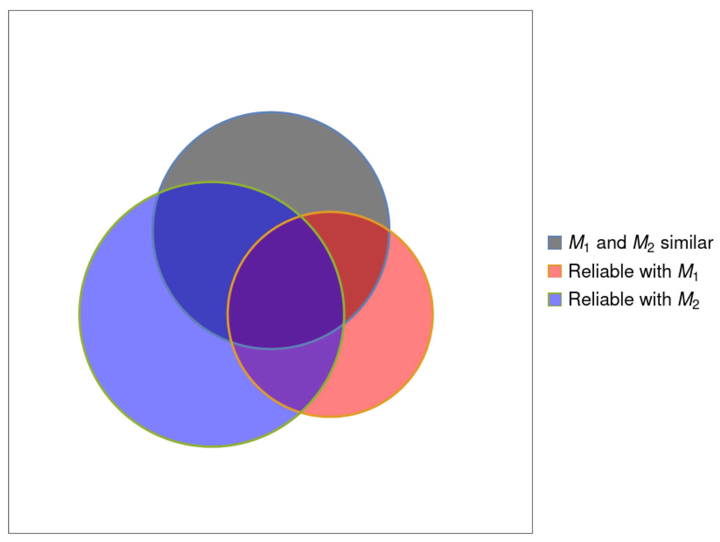
• N, the number of systems in the data set (corresponding to the white square in Figure 1).
• $N_s(M_1,M_2,\dots ;{ϵ}_s)$, or $N_s\left({ϵ}_s\right)$ for brevity, the number of systems that yield similar results (within ${ϵ}_s$) using methods $M_1,M_2,\dots$. (corresponding to the gray disk in Figure 1).
• $N_r(M,{ϵ}_r)$, the number of systems for which method M is reliable (corresponding to the red or blue disk in Figure 1).
• $N_r(M,{ϵ}_r\cap {ϵ}_s)$, the number of systems for which method M is reliable and similar to the other methods (corresponding to the overlap region of the three disks in Figure 1).

2.3. Probabilities

If the data set is sufficiently large, we can estimate probabilities as frequencies from these numbers:

• The probability to obtain a reliable result with method M,

  $$P_r(M,{ϵ}_r)=\frac{N_r(M,{ϵ}_r)}{N}$$

  (4)
• The probability to obtain similar results for the set of considered methods,

  $$P_s(M_1,M_2,\dots ;{ϵ}_s)=P_s\left({ϵ}_s\right)=\frac{N_s\left({ϵ}_s\right)}{N}$$

  (5)
  For a finite sample, the smallest value of ${ϵ}_s$ for which $P_s\left({ϵ}_s\right)=1$ is called the Hausdorff distance [4].
• The (conditional) probability to obtain reliable results with method M, given that this method is similar to the other methods in the set,

  $$P_{r|s}(M,{ϵ}_r,{ϵ}_s)=\frac{N_r(M,{ϵ}_r\cap {ϵ}_s)}{N_s\left({ϵ}_s\right)}$$

  (6)
• The (conditional) probability that a result with method M is similar to that of the other methods, given that it is reliable,

  $$P_{s|r}(M,{ϵ}_s,{ϵ}_r)=\frac{N_r(M,{ϵ}_r\cap {ϵ}_s)}{N_r(M,{ϵ}_r)}$$

  (7)

with the limit values

$$\begin{array}{ccc}\hfill P_{r|s}(M,{ϵ}_r=\infty ,{ϵ}_s)& =& P_s\left({ϵ}_s\right)\hfill \end{array}$$

(8)

$$\begin{array}{ccc}\hfill P_{r|s}(M,{ϵ}_r,{ϵ}_s=\infty )& =& P_r(M,{ϵ}_r)\hfill \end{array}$$

(9)

$$\begin{array}{ccc}\hfill P_{s|r}(M,{ϵ}_s=\infty ,{ϵ}_r)& =& 1\hfill \end{array}$$

(10)

$$\begin{array}{ccc}\hfill P_{s|r}(M,{ϵ}_s,{ϵ}_r=\infty )& =& P_s\left({ϵ}_s\right)\hfill \end{array}$$

(11)

Furthermore, even for ${ϵ}_s={ϵ}_r=ϵ$, in general, $P_s\left(ϵ\right)\ne P_r(M,ϵ)$ and $P_{s|r}(M,ϵ)\ne P_{r|s}(M,ϵ)$, where the notations were shortened to imply the equality of both thresholds.

The main objective of this paper is to investigate whether choosing methods with similar results is a good criterion of reliability, i.e., to what extent $P_{r|s}({ϵ}_r,{ϵ}_s)P_r\left({ϵ}_r\right)$. Even if this aim is achieved, this does not go without a drawback: the systems for which similarity is not reached are eliminated from the study with a probability $1-P_s\left({ϵ}_s\right)$. $P_{s|r}(M,{ϵ}_s,{ϵ}_r)$ gives us an indication about the quality of our selection criteria by similarity.

An important limitation of this approach is the sample size. Even for large data sets, it may happen that the number of similar results, $N_s\left({ϵ}_s\right)$ is small, e.g., because at least one of the methods yields results systematically different from that of the other methods or because ${ϵ}_s$ was chosen too small. In such a case, the uncertainty of the empirical estimates becomes large.

2.4. Statistical Measures

Often, the distribution of errors is summarized by numbers, such as the mean error, the mean absolute error, and the standard deviation. Although these numbers convey some information, they sometimes hide the misconception that the distribution of errors is normal. In the cases we analyze below, as in most cases we studied previously [5], the distributions of errors are not normal. This justifies the use of probabilistic estimators, such as those presented in our previous work [1,2,3], or the ones introduced here.

A direct link can be made between the statistics based on the empirical cumulative distribution function (ECDF) of the absolute errors, presented in ref. [3], and some of those introduced above:

• The reliability probability $P_r(M,{ϵ}_r)$ is equivalent to the ECDF of the absolute errors, noted $C\left(ϵ\right)$ in our previous work.
• The qth percentile $Q_q\left(M\right)$ of the absolute errors is the value of ${ϵ}_r$, such as $P_r(M,{ϵ}_r)=q/100$.

The conditional probabilities $P_{r|s}(M,ϵ)$ and $P_{s|r}(M,ϵ)$ will, thus, be represented as conditional ECDFs as a function of $ϵ$, generalizing our former probabilistic statistics.

3. Applications

3.1. Guidelines

In order to obtain a better understanding of the situations arising from data extracted from the chemical literature, let us first consider pairs of points generated randomly according to normal distributions: each point is assimilated to a “system”, where the values on the abscissa are interpreted as “errors” for $M_1$ while those on the ordinate as “errors” for $M_2$. The results are presented in Figure 2. The panels on the left show the randomly produced “errors” (green dots).

The red stripe shows the reliability region for $M_1$, where $\left|E\right(M_1,S|{ϵ}_r$ (cf. Equation (2)), and the blue stripe shows the same for $M_2$. The gray stripe shows the region where the results produced by $M_1$ and $M_2$ are within $\pm {ϵ}_s$ (Equation (3)). Some points are marked by numbers. The polygon with corners corresponding to the points (2, 4, 6, and 8) delimits the region where $M_1$ is both close to $M_2$ and is reliable. The polygon with corners corresponding to the points (1, 3, 5, and 7) delimits the region where $M_2$ is both close to $M_1$ and is reliable. The plots were drawn by choosing ${ϵ}_r={ϵ}_s=1$.

The ratio of the number of points in the red or blue stripe to the total number of points gives $P_r$. The ratio of the number of points in the gray stripe to the total number of points gives $P_s$. The ratio the number of points in the polygons (1, 3, 5, and 7) or (2, 4, 6, and 8) to the number of points in the gray stripe gives $P_{r|s}$. The ratio the number of points in the polygons to those in the red or blue stripe give $P_{s|r}$. The panels on the right show the dependence of the probabilities on ${ϵ}_r={ϵ}_s$. The results for $M_1$ are in blue, those for $M_2$ in red. $P_r\left(M_i\right)$ are drawn as thin curves, $P_{r|s}$ as thick curves, and those for $P_{r|s}$ as dashed curves.

The top row is produced for errors centered at the origin (the mean errors are equal to zero for both methods; the variance is different for the two methods). In the second row, the mean errors are different and non-zero. In the third row, a correlation is introduced between the errors produced by the two methods. In the last row, the effect of correlation is enhanced. In the first three rows, the parameters are inspired from those obtained for the PBE/HSE06 pair (see Section 3.2), in the last row different parameters are used, namely those of PBE0/HSE06.

Let us start by discussing the first row. We see that, from the choice made for ${ϵ}_r$ and ${ϵ}_s$, an important number of points is in the region where $|E(M_i,S)|{ϵ}_r$, ($i=1,\mathrm{or}2$) and $|E(M_1,S)-E(M_2,S)|{ϵ}_s$. However, there are points that are within the reliable range for both methods (in the region where the red and blue stripes overlap) are not within the region of similarity (gray stripe).

This could be corrected by increasing ${ϵ}_s$ to $\sqrt{2}{ϵ}_r$, but there is a price to pay for it: for each of the methods, the number of points selected increases by including systems for which the method does not yield reliable results. Furthermore, we notice that there are points that are reliable with one method but not similar to the other method. There are also points that are similar but unreliable (inside the gray stripe but outside either the red or the blue stripe). Finally, there are points that where the methods are both unreliable and dissimilar (on white background). Let us now look at the evolution of probabilities with ${ϵ}_r={ϵ}_s$ (top right panel). We see that $M_1$ is globally of worse quality than $M_2$, as $P_r\left(M_1\right)P_r\left(M_2\right)$ (thin curves).

When first selecting the results by similarity and then checking the reliability, we see that the conditional probabilities $P_{r|s}$ are close for $M_1$ and $M_2$ and better than the $P_r$ curves. Checking similarity has eliminated part of the good results (that were reliable with either $M_1$ or $M_2$) but provides a higher probability to obtain a good result. Note that, while $P_{r|s}$ is slightly better for $M_2$ than for $M_1$, the inverse is true for $P_{s|r}$, a consequence of the division by $P_r$.

Let us now shift the point cloud by analyzing it for the case when the mean errors are non-zero. If the shift for at least one of the methods is important, none of the “systems” produces similar results for the two methods (the point cloud is shifted outside the gray stripe). The figure shows an intermediate case, where the shift is not so important and plays a role mainly for $M_1$.

The similarity (gray stripe) essentially retains the results that are good for $M_2$ (within the blue stripe) because the number of points that are both similar and reliable for $M_1$ is reduced. As a result (second row, right panel), the similarity hardly improves the probability to obtain a good result for the better method ($M_2$) but eliminates a number of systems for which $M_2$ would provide reliable results. However, there is still an improvement for the method of lower quality ($M_1$).

Another effect reducing the improvement is the existence of positive correlation between the “errors”. This is exemplified in the last two rows, where the position of the points are concentrated around a line. In the limit of perfect correlation, these points lie all on a line. If the mean errors make the lines lie in the similarity region, $P_{r|s}=P_r$: no gain is obtained through similarity. If the line lies outside the similarity region (outside the gray stripe), even worse, no point is selected by similarity: if we rely on similarity only, we cannot use any of the calculations.

Note that the correlation between data produces an increase in $P_{s|r}$: if a method is producing a reliable result, by correlation, it is likely that the other method produces also a reliable result, except when one of the methods is strongly biased compared to the other.

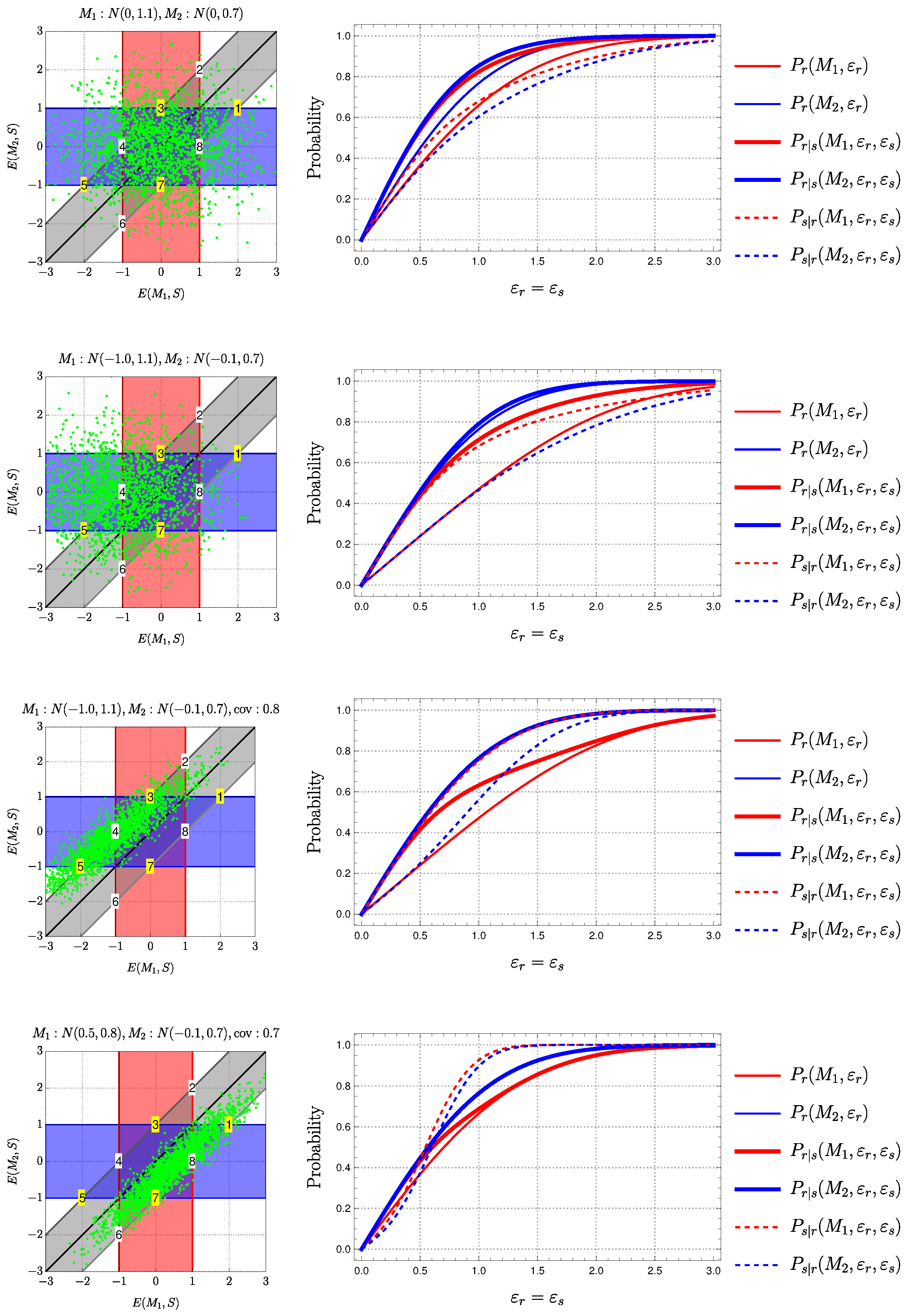
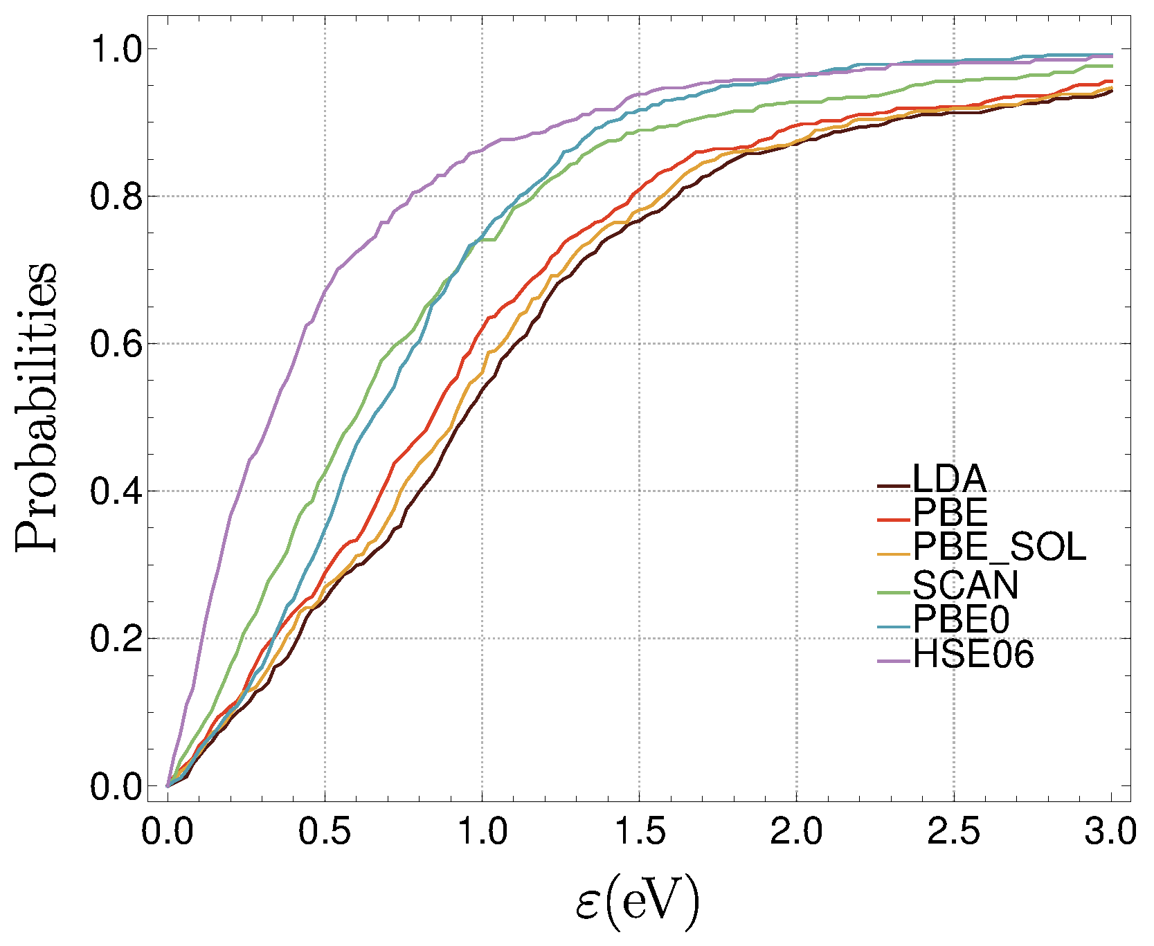
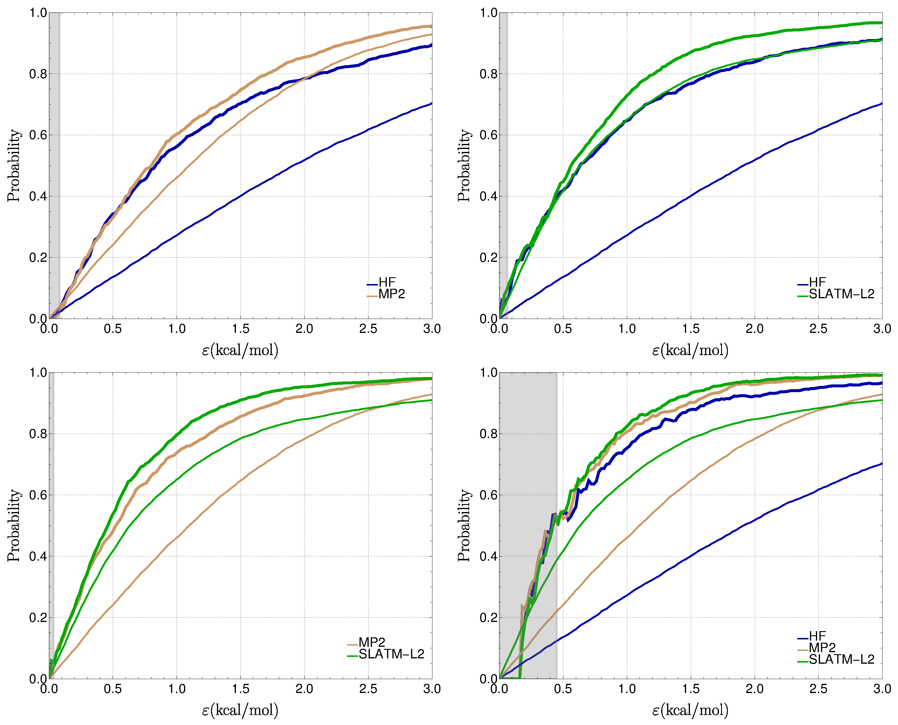
3.2. The BOR2019 Dataset

We consider a set of band gaps obtained for 471 systems with a selected set of density functional approximations (DFAs): LDA [6,7], PBE [8], PBEsol [9], SCAN [10], PBE0 [11,12], and HSE06 [13,14]. All the data were taken from Borlido et al. [15], and most summary statistics referred to below were reported in a previous study [1,2] (case BOR2019).

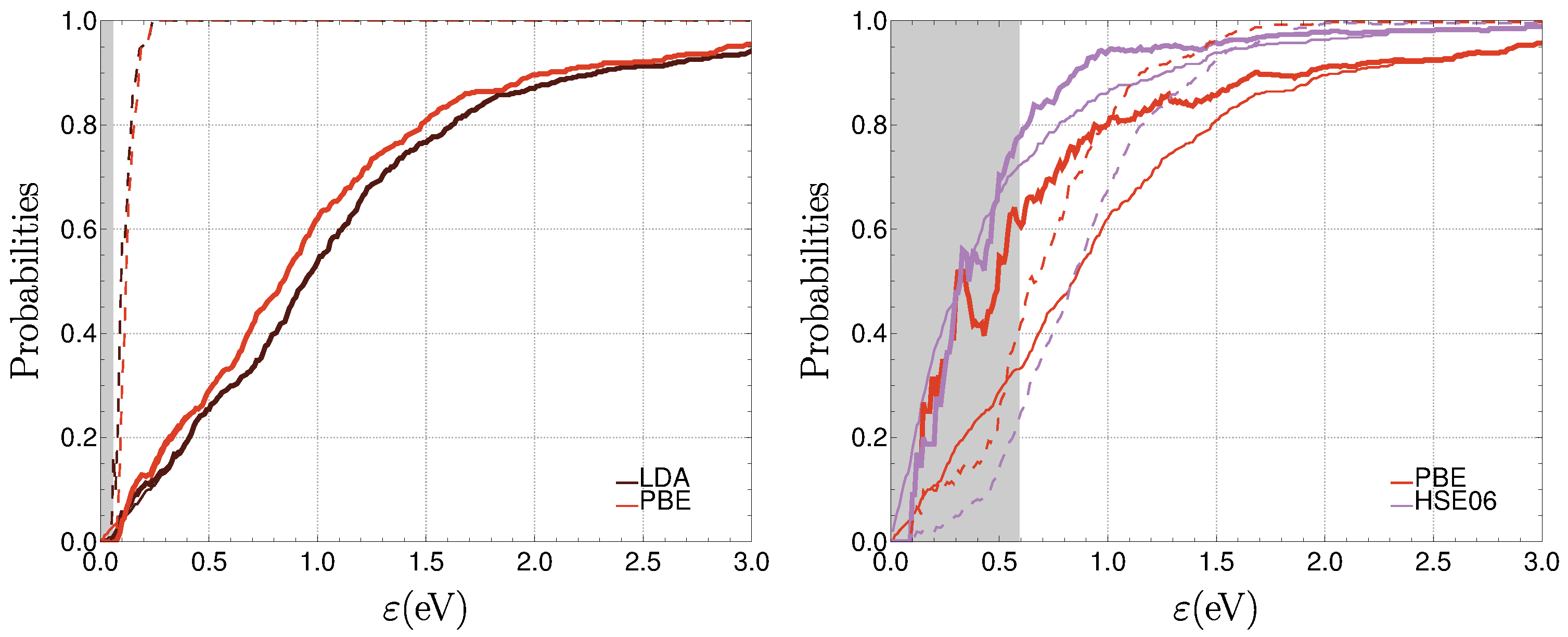
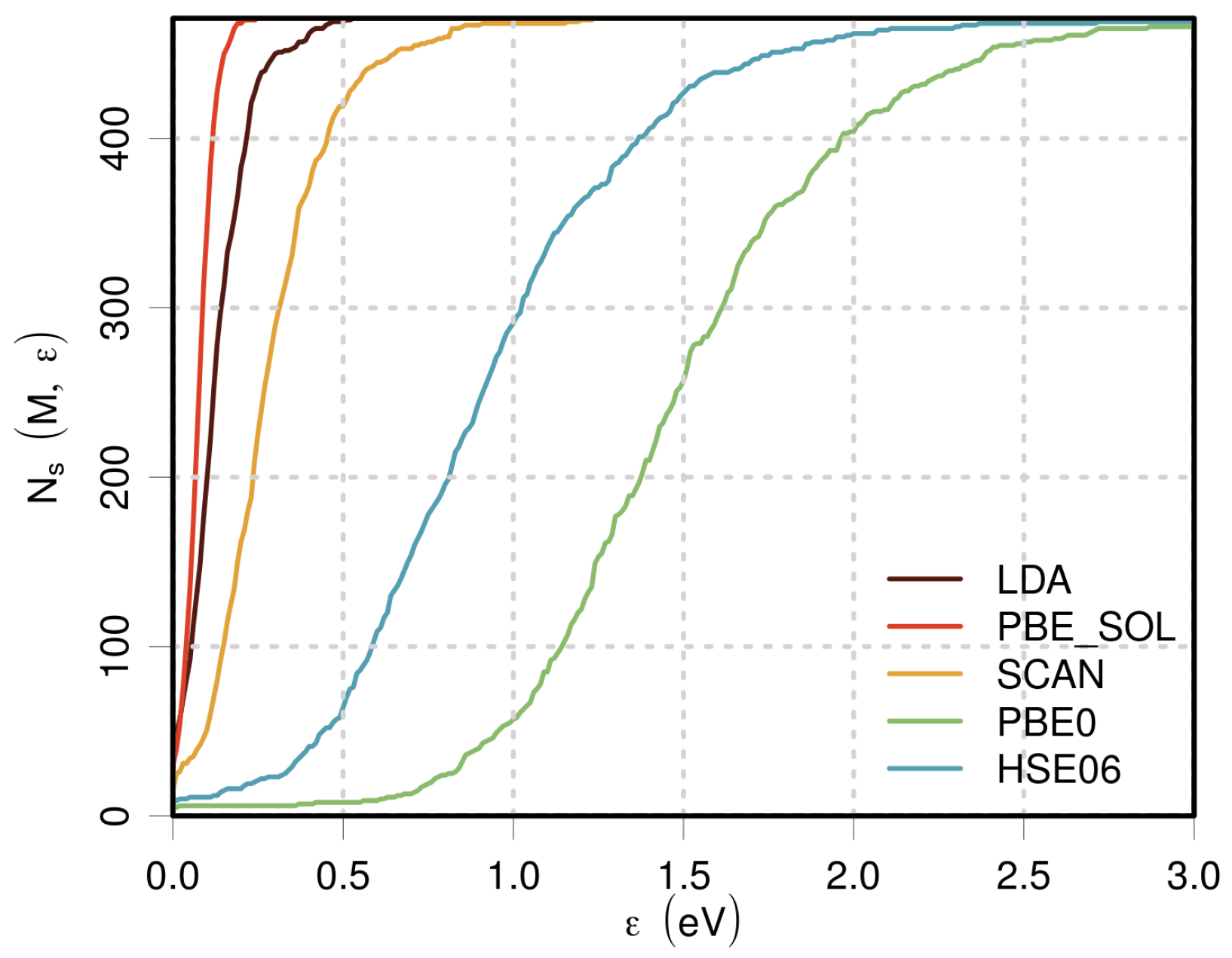
3.2.1. Performance of Individual Methods

The errors in the band gaps are quite large for this set of methods. The mean absolute errors lie between 0.5 eV (HSE06) and 1.2 eV (LDA), while $Q_{95}$ varies between 1.7 eV (HSE06) and 3.2 eV (LDA) (Figure 3). The probability to have more reliable than unreliable results occurs at the median absolute error, which defines a minimal value ${ϵ}_r=0.33$ eV for HSE06—the best method in this set.

Figure 3 shows the dependence of $P_r(M,ϵ)$ on $ϵ$. One can can safely qualify HSE06 as the best (most reliable) among the methods as $P_r(\mathrm{HSE}06,ϵ)$ is never smaller than any of the other $P_r(M,ϵ)$ curves (within the sampling uncertainty). While PBE0 becomes competitive with HSE06 for $ϵ1.7$ eV, it behaves rather like SCAN for the values of $ϵ\approx 1$ eV and like the group of the three methods that perform worst (LDA, PBE, and PBEsol) for small $ϵ$ values.

It is important to have in mind that, even if PBE0 and SCAN are identically reliable at the $ϵ=1$ threshold ($P_r(\mathrm{PBE}0,ϵ=1)\simeq P_r(\mathrm{SCAN},ϵ=1)$), this is not necessarily true for the same subset of systems.

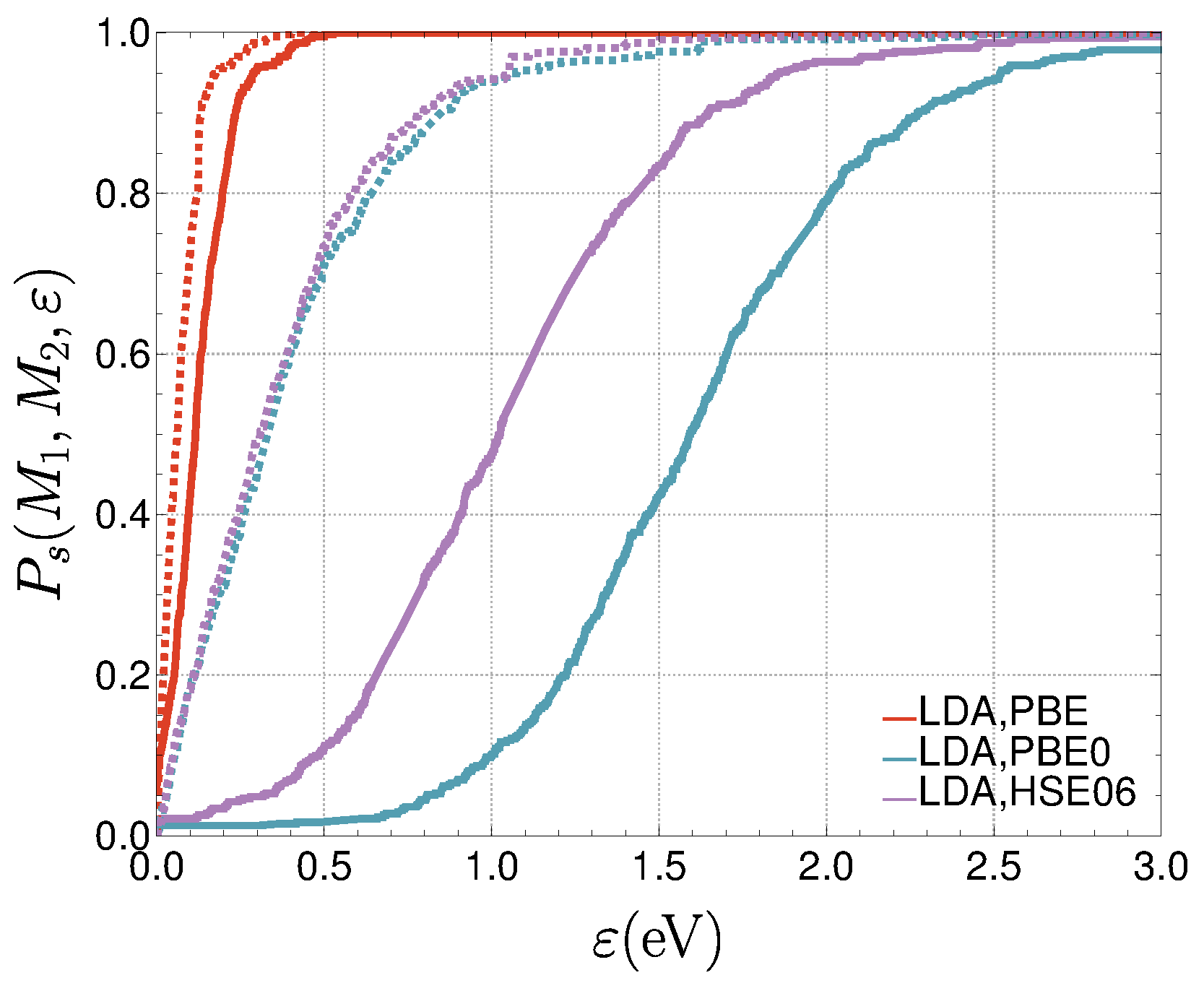
3.2.2. Similarity and Reliability

Figure 4 shows the absolute errors made by two methods (HSE06 and PBE or PBE0) and the distance between the results obtained with the two methods. We choose, for example, a threshold for the similarity of the two methods, ${ϵ}_s=1$ eV. We take the same value for the threshold defining a method reliable, ${ϵ}_r=1$ eV.

If we assume that the similarity of the results is a good criterion to select the reliable results, the points should lie either in the bottom left rectangle ($|X(M_1,S)-X(M_2,S)|{ϵ}_s,\left|E(M,S)\right|{ϵ}_r$), meaning that the selected results are reliable, or in the top right rectangle ($|X(M_1,S)-X(M_2,S)|{ϵ}_s,\left|E(M,S)\right|{ϵ}_r$), meaning that dissimilarity eliminates the bad results. However, we see many points in the top left rectangle ($|X(M_1,S)-X(M_2,S)|{ϵ}_s,\left|E(M,S)\right|{ϵ}_r$), showing that it is possible that similar results should be rejected.

This naturally shows up when the methods are highly correlated, as it is the case for HSE06 and PBE0. Furthermore, we notice the presence of points in the bottom right rectangle ($|X(M_1,S)-X(M_2,S)|{ϵ}_s,\left|E(M,S)\right|{ϵ}_r$), especially for the HSE06/PBE pair, indicating that the similarity criterion has eliminated good results obtained with one of the methods.

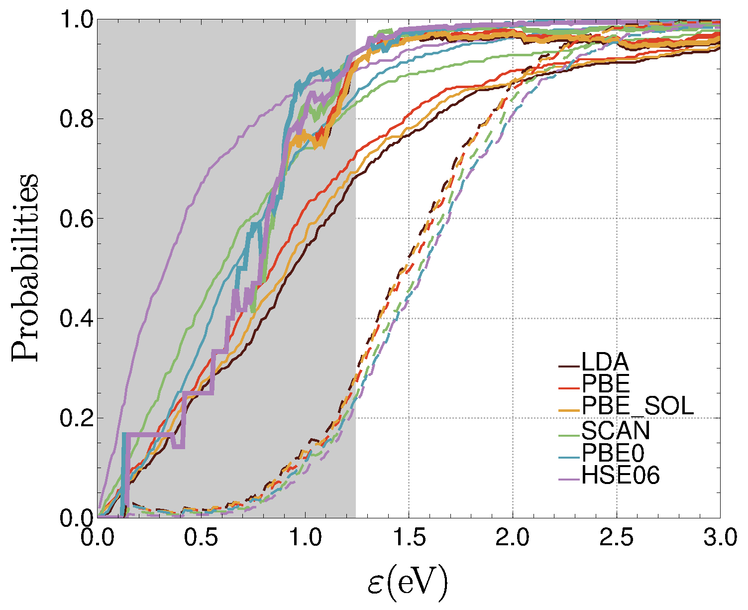
3.2.3. Impact of Similarity on Reliability

Let us now look at the probabilities as functions of $ϵ$ (we take ${ϵ}_s={ϵ}_r=ϵ$), Figure 5. As a reference, we plot $P_r(M,ϵ)$ (thin curves, identical to the ECDF curves in Figure 3), the estimation of reliability when no similarity check is made. The thick curves correspond to $P_{r|s}(M,ϵ)$, the probability to obtain with method M errors smaller than $ϵ$ if the results of method M are within $\pm ϵ$ of the other method(s). The dashed curves indicate $P_{s|r}(M,ϵ)$, the probability of a reliable result obtained with method M to be in the subset selected by similarity.

The data set contains originally 471 systems. However, by making selections, e.g., of systems where the DFAs yield similar results, the size of the sample is reduced, and the use of statistical estimates is hampered. We estimate that, below 100 selected systems, the statistics become unreliable. The region for which the size of the sample is smaller than 100 is marked by a gray rectangle in Figure 5.

We notice that, for LDA and PBE, which provide close reliability curves, practically no distinction can be made between the thin and thick curves: similarity has no impact on reliability. We also see that $P_{s|r}(M,ϵ)\approx 1$ for almost the whole range of $ϵ$: if one method gives a reliable result for a system, the other one is very likely to give a reliable result too. Thus, the size of the sample of similar results is reaching a size comparable to that of the complete sample already for a small value of $ϵ$ (the gray rectangle is very thin).

The situation changes when we compare PBE to HSE06. The region where the size of the sample of similar results is below 100 reaches a large value of $ϵ\approx 0.6$ eV. For $ϵ0.6$ eV, we notice an improvement for each of the methods: $P_{r|s}(M,ϵ)P_r(M,ϵ)$. However, we notice that the improvement of the worse of the two methods is not compensating the difference of quality between the two methods.

Even as $ϵ$ increases beyond 0.6 eV, $P_{s|r}(M,ϵ)$ is at first relatively small: if one method gives a reliable result, the probability that the other provides a reliable result too, is relatively small. Without surprise, the risk of the better of the two methods (HSE06) to eliminate systems by selection is higher than that of the worse of the two methods (PBE), cf. dashed curves in Figure 5. In this case, one should take the result provided by the better of the two methods, not, e.g., the average of the results of the two methods.

The improvement has to be paid: for some of the systems, the methods provide results that are not similar, and are not taken into consideration - we have no answer to give for these systems. Figure 6 shows an example by choosing PBE, finding how many systems from the data set are similar (within $ϵ$) to those obtained with another method. The graph confirms that an important number of systems are lost, unless one declares similarity by choosing a large value for $ϵ$.

Let us attempt to condensate the results by looking at the values of $ϵ$ for which the probabilities of having an absolute error smaller than $ϵ$ is 0.95, $Q_{95}\left(M\right)$, cf.

Table 1. $Q_{95}\left(M_1\right)$, in eV, for the method indicated by the row ($M_1$), when similar to the method described by the column ($M_2$), for ${ϵ}_s={ϵ}_r$.

${\mathit{M}}_1\setminus {\mathit{M}}_2$	LDA	PBE	PBEsol	SCAN	PBE0	HSE06
LDA	3.1	3.1	3.1	3.1	2.1	3.1
PBE	2.9	2.9	2.9	2.9	2.1	2.9
PBEsol	3.0	3.0	3.0	3.0	2.2	3.0
SCAN	2.4	2.4	2.4	2.4	2.1	2.4
PBE0	1.4	1.4	1.4	1.5	1.8	1.8
HSE06	1.1	1.3	1.1	1.7	1.7	1.7

. This provides only an exploration of the behavior at large $ϵ$. Nevertheless, it leads to the conclusions above: LDA and PBE do not gain by using similarity: $Q_{95}\left(\mathrm{LDA}\right)=3.1$ eV and $Q_{95}\left(\mathrm{PBE}\right)=2.9$ eV, even after similarity is imposed. However, $Q_{95}\left(\mathrm{HSE}06\right)$ decreases from 1.7 to 1.3 eV when the similarity with PBE is taken into account.

We can expect the errors of different DFAs to be highly correlated [2]. (For example, recall that making the approximation valid for the uniform electron gas is a basic ingredient in almost all DFAs.) In other words, this could mean that if one method is right, all are right, and if one method is wrong, all are wrong: little improvement can be expected from agreement between methods.

Another measure of similarity is Spearman’s rank correlation coefficient (

Table 2. Rank correlation matrix between error sets.

${\mathit{M}}_1\setminus {\mathit{M}}_2$	LDA	PBE	PBEsol	SCAN	PBE0	HSE06
LDA	1	0.99	1.00	0.95	0.76	0.81
PBE	-	1	1.00	0.97	0.78	0.83
PBEsol	-	-	1	0.96	0.77	0.82
SCAN	-	-	-	1	0.83	0.87
PBE0	-	-	-	-	1	0.98
HSE06	-	-	-	-	-	1

). This varies between 0.76 (LDA and PBE0), and 0.99/1.00 (within the group of lower performance: LDA, PBE, and PBEsol). For PBE and HSE06, it takes an intermediate value (0.83). The correlation coefficients gives a hint for grouping the methods; however, it is more difficult to extract from them the information given in Figure 5 than it is from $Q_{95}\left(M\right)$.

Another problem of using the correlation index is its invariance with respect to a monotonous transformation of the calculated values (a linear transformation for the Pearson correlation). If one of the methods is biased and another not, these methods are not likely to give similar results, despite a high correlation index. Of course, this dissimilarity can be reduced by correcting the bias, typically, by subtracting the estimated mean error from the values obtained.

Figure 7 shows the probability that the results of two methods are similar (within $ϵ$). The similarity of LDA and PBE can be recognized immediately, as well as the dissimilarity between LDA and PBE0 or HSE06. One can also notice the improvement after centering the errors (i.e., correcting the bias by subtracting the mean signed error for each of the methods). At the same time, the difference between methods (PBE0 and HSE06) is reduced.

One may want to summarize the information present in $P_s(M_1,M_2;ϵ)$ by its mean, ${\mu }_s(M_1,M_2)$, and standard deviation, ${\sigma }_s(M_1,M_2)$:

$$\begin{array}{ccc}\hfill {\mu }_s(M_1,M_2)& =& {\int }_0^{\infty }ϵ[1-P_s(M_1,M_2;ϵ)]dϵ\hfill \end{array}$$

(12)

$$\begin{array}{ccc}\hfill {\sigma }_s^2(M_1,M_2)& =& {\int }_0^{\infty }{ϵ}^2[1-P_s(M_1,M_2;ϵ)]dϵ-{\mu }_s^2\hfill \end{array}$$

(13)

The numerical results are given in

Table 3. The mean and the standard deviation of the probability distribution of having two DFAs giving similar results, ${\mu }_s(M_1,M_2)\left({\sigma }_s(M_1,M_2)\right)$, Equations (12) and (13).

${\mathit{M}}_1\setminus {\mathit{M}}_2$	LDA	PBE	PBEsol	SCAN	PBE0
PBE	0.1(0.1)	-	-	-	-
PBEsol	0.1(0.1)	0.1(0.0)	-	-	-
SCAN	0.4(0.3)	0.3(0.2)	0.4(0.2)	-	-
PBE0	1.6(0.6)	1.5(0.5)	1.6(0.5)	1.2(0.4)	-
HSE06	1.1(0.5)	0.9(0.5)	1.0(0.5)	0.6(0.3)	0.6(0.2)

. The similarity of LDA, PBE, and PBEsol is well visible from these numbers.

Let us now increase the number of methods that we are considering. Taking into account the closeness of the results of LDA, PBE, and PBEsol, we do not expect anything considering the similarity of these three methods. However, one might ask whether comparing PBE, HSE06, and SCAN, or PBE, HSE06, and PBE0 provides any improvement. In the first case, $Q_{95}\left(\mathrm{HSE}06\right)$ stays at 1.3 eV; in the second, it slightly increases to 1.4 eV.

Increasing the number of methods for similarity checks does not provide necessarily an improvement on reliability (as one increases the number of “bad” methods to compare with). All six methods provides, at best, $Q_{95}\left(M\right)\approx 1.3$ eV, while the best value in Table 1 is of 1.1 eV. This can be also seen in Figure 8, the analogue of Figure 5, showing the probabilities obtained when similarity among all six methods is taken into account. This also shows the increase of the region of poor sampling.

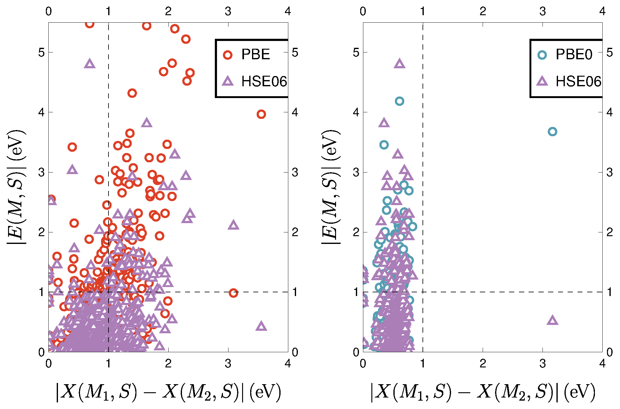
3.2.4. Eliminating Strange Results?

The distribution of errors in density functional approximations is often not normal [5]. This can be seen in Figure 9. It seems that similarity confirms (in part) the prejudice that a strange behavior of one method is not repeated by another, different method. After restricting the data set to similar values, the distribution of errors is more compact. This explains the lowering of the $Q_{95}\left(M\right)$. Recall, however, that wrong results obtained with both methods are not excluded.

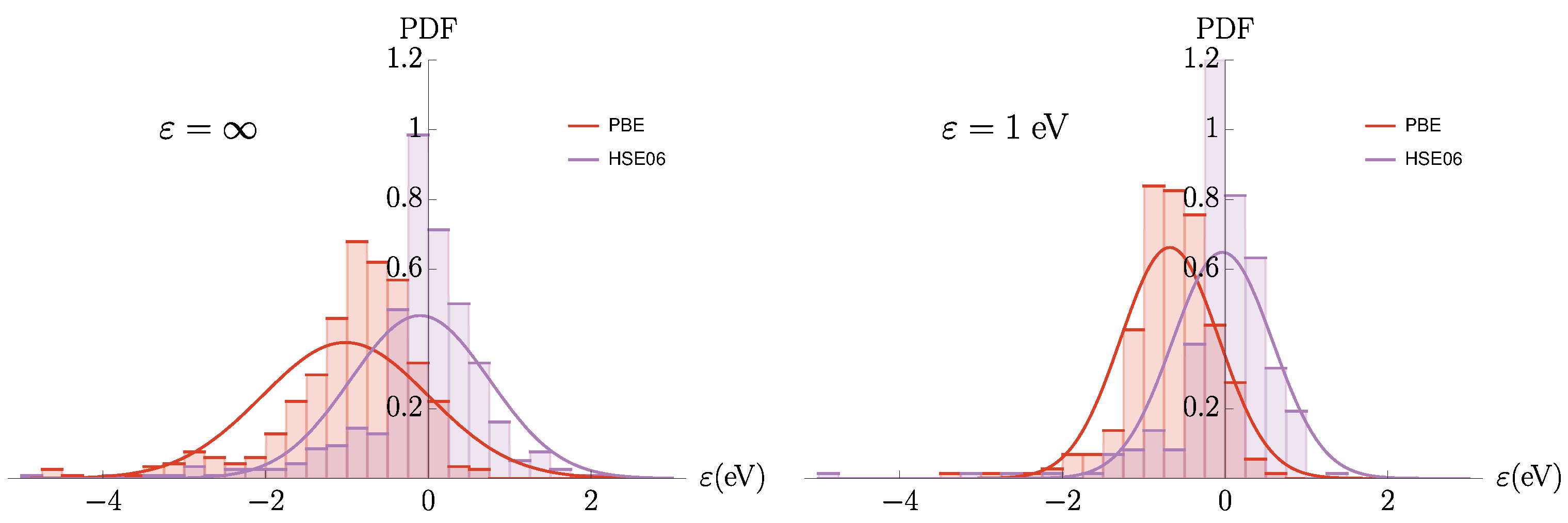
3.3. The ZAS2019 Dataset

The effective atomization energies (EAE) for the QM7b dataset [16], for molecules up to seven heavy atoms (C, N, O, S, and Cl) are issued from the study by Zaspel et al. [17]. We consider here values for the cc-pVDZ basis set, and the prediction error for 6211 systems for the SCF, MP2, and machine-learning (SLATM-L2) methods with respect to CCSD(T) values as analyzed by Pernot et al. [18].

In contrast to the case of the DFAs presented in the previous section (Table 2), the errors in this dataset present negligible rank correlation coefficients (smaller than 0.1 in absolute value). Similarity will, thus, be dominated by the bias in the errors and their dispersion. The $P_r(M,ϵ)$ and $P_{r|s}(M,ϵ)$ curves are shown in Figure 10. When comparing HF to MP2, one sees that both methods benefit from similarity as soon as $ϵ0.2$ kcal/mol.

Naturally, HF benefits much more from the similarity selection than MP2: its $Q_{95}$ decreases from 6.1 to 4.2 kcal/mol, while $Q_{95}$ for MP2 decreases slightly from 3.4 to 2.9 kcal/mol. A similar behavior is observed in the comparison of HF to SLATM-L2 with a larger onset of improvement for SLATM-L2 ($ϵ\sim 0.5$ kcal/mol). For HF, $Q_{95}$ decreases from 6.1 to 3.8 kcal/mol and for SLATM-L2 from 4.7 to 2.5 kcal/mol. The comparison of MP2 to SLATM-L2 provides an intermediate case, where both methods present more balanced improvements: for MP2, $Q_{95}$ decreases from 3.4 to 2.4 kcal/mol and for SLATM-L2 from 4.7 to 1.9 kcal/mol.

Adding HF to the MP2/SLATM-L2 pair produces a marginal gain for the latter methods, whereas HF presents a strong gain in reliability: the final $Q_{95}$ values are 2.5 (HF), 1.8 (MP2) and 1.7 kcal/mol (SLATM-L2). However, this comes at the price of a large number of system rejections: for $ϵ\sim 2.0$ kcal/mol, only 1/4th of the 6211 systems are selected by their similarity. For comparison, this number is about 2/3rd for the MP2/SLATM-L2 comparison.

In this context of uncorrelated error sets with different accuracy levels, one sees that similarity selection has a notable positive impact on the reliability of predictions by any of the methods, even the most accurate ones. It is striking that MP2 or SLATM-L2 might benefit from comparison with HF, but, as already discussed for band gaps (Figure 9), this proceeds mainly by elimination of systems with large errors.

4. Conclusions

We asked whether picking only results that are similar to different methods would improve the accuracy of their predictions (in spite of possibly eliminating a significant part of the calculations done). The use of probabilities to treat reliability and similarity was illustrated on two benchmark data sets, one of band gap calculations with different density functional approximations, the other of effective atomization energies with two ab initio methods and one machine-learning method.

For the properties and methods studied, the thresholds for reliability and similarity were chosen quite generously. For the band gap data set, we found that similarity of the density functional results had only a marginal impact on improving the prediction accuracy. This is consistent with previous findings that the differences between density functional approximations are less important when considering the error distributions [1,2], or taking into account experimental uncertainty [19].

For the effective atomization energies data set, in which the error sets are uncorrelated, notable improvements of reliability after similarity selection were observed for all methods, even the most accurate ones. Roughly, we observed two categories of results:

• methods that always give close results, for which similarity is irrelevant; and
• methods for which an improvement can be achieved, especially by eliminating certain systems that behave strangely with one or the other methods—similarity is mainly effective for eliminating large errors.

Note that the size of the data sets might have an impact on the uncertainty of all the statistics. For the smaller datasets, this uncertainty might be comparable with the observed differences between statistics. Bootstrapping approaches, such as the ones used in our previous works [1,3], could be used to this effect. This was not the focus of the present study, and uncertainty management will be considered in forthcoming research.

References

1. Pernot, P.; Savin, A. Probabilistic performance estimators for computational chemistry methods: Systematic Improvement Probability and Ranking Probability Matrix. I. Theory. J. Chem. Phys. 2020, 152, 164108. [Google Scholar] [CrossRef] [PubMed]
2. Pernot, P.; Savin, A. Probabilistic performance estimators for computational chemistry methods: Systematic Improvement Probability and Ranking Probability Matrix. II. Applications. J. Chem. Phys. 2020, 152, 164109. [Google Scholar] [CrossRef] [PubMed]
3. Pernot, P.; Savin, A. Probabilistic performance estimators for computational chemistry methods: The empirical cumulative distribution function of absolute errors. J. Chem. Phys. 2018, 148, 241707, Erratun in J. Chem. Phys. 2019, 150, 219906. [Google Scholar] [CrossRef] [PubMed] [Green Version]
4. Hausdorff, F. Set Theory; Chelsea: London, UK, 1978. [Google Scholar]
5. Pernot, P.; Savin, A. Using the Gini coefficient to characterize the shape of computational chemistry error distributions. Theor. Chem. Acc. 2021, 140, 24. [Google Scholar] [CrossRef]
6. Dirac, P.A.M. Note on Exchange Phenomena in the Thomas Atom. Math. Proc. Camb. Philos. Soc. 1930, 26, 376–385. [Google Scholar] [CrossRef] [Green Version]
7. Vosko, S.H.; Wilk, L.; Nusair, M. Accurate spin-dependent electron liquid correlation energies for local spin density calculations: A critical analysis. Can. J. Phys. 1981, 58, 1200–1211. [Google Scholar] [CrossRef] [Green Version]
8. Perdew, J.P.; Burke, K.; Ernzerhof, M. Generalized Gradient Approximation Made Simple. Phys. Rev. Lett. 1996, 77, 3865–3868. [Google Scholar] [CrossRef] [PubMed] [Green Version]
9. Perdew, J.P.; Ruzsinszky, A.; Csonka, G.I.; Vydrov, O.A.; Scuseria, G.E.; Constantin, L.A.; Zhou, X.; Burke, K. Restoring the Density-Gradient Expansion for Exchange in Solids and Surfaces. Phys. Rev. Lett. 2008, 100, 136406, Erratun in Phys. Rev. Lett. 2009, 102, 039902. [Google Scholar] [CrossRef] [PubMed]
10. Zhang, Y.; Kitchaev, D.A.; Yang, J.; Chen, T.; Dacek, S.T.; Sarmiento-Perez, R.A.; Marques, M.A.L.; Peng, H.; Ceder, G.; Perdew, J.P.; et al. Efficient first-principles prediction of solid stability: Towards chemical accuracy. Npj Comput. Mater. 2018, 4, 9. [Google Scholar] [CrossRef]
11. Perdew, J.P.; Ernzerhof, M.; Burke, K. Rationale for mixing exact exchange with density functional approximations. J. Chem. Phys. 1996, 105, 9982–9985. [Google Scholar] [CrossRef]
12. Adamo, C.; Barone, V. Toward reliable density functional methods without adjustable parameters: The PBE0 model. J. Chem. Phys. 1999, 110, 6158–6170. [Google Scholar] [CrossRef]
13. Heyd, J.; Scuseria, G.E.; Ernzerhof, M. Hybrid functionals based on a screened Coulomb potential. J. Chem. Phys. 2003, 118, 8207–8215, Erratun in J. Chem. Phys. 2006, 124, 219906. [Google Scholar] [CrossRef] [Green Version]
14. Krukau, A.V.; Vydrov, O.A.; Izmaylov, A.F.; Scuseria, G.E. Influence of the exchange screening parameter on the performance of screened hybrid functionals. J. Chem. Phys. 2006, 125, 224106. [Google Scholar] [CrossRef] [PubMed]
15. Borlido, P.; Aull, T.; Huran, A.W.; Tran, F.; Marques, M.A.L.; Botti, S. Large-scale benchmark of exchange-correlation functionals for the determination of electronic band gaps of solids. J. Chem. Theor. Comput. 2019, 15, 5069–5079. [Google Scholar] [CrossRef] [PubMed] [Green Version]
16. Montavon, G.; Rupp, M.; Gobre, V.; Vazquez-Mayagoitia, A.; Hansen, K.; Tkatchenko, A.; Müller, K.R.; Anatole von Lilienfeld, O. Machine learning of molecular electronic properties in chemical compound space. New J. Phys. 2013, 15, 095003. [Google Scholar] [CrossRef]
17. Zaspel, P.; Huang, B.; Harbrecht, H.; von Lilienfeld, O.A. Boosting Quantum Machine Learning Models with a Multilevel Combination Technique: Pople Diagrams Revisited. J. Chem. Theory Comput. 2019, 15, 1546–1559. [Google Scholar] [CrossRef] [PubMed] [Green Version]
18. Pernot, P.; Huang, B.; Savin, A. Impact of non-normal error distributions on the benchmarking and ranking of Quantum Machine Learning models. Mach. Learn. Sci. Technol. 2020, 1, 035011. [Google Scholar] [CrossRef]
19. Savin, A.; Pernot, P. Acknowledging User Requirements for Accuracy in Computational Chemistry Benchmarks. Z. Anorg. Allg. Chem. 2020, 646, 1042–1045. [Google Scholar] [CrossRef]
Figure 1. A schematic representation of the properties of the systems. The region within the square represents the set of all benchmark systems. The red disk represents the set of systems for which method M 1 is reliable. The blue disk represents the set of systems for which method M 2 is reliable. The gray disk represents the set of systems for which methods M 1 and M 2 give similar results.
Computation 10 00027 g001
Figure 2. Examples of reliability and similarity configurations (left) and the corresponding probability curves (right) for two error sets sampled from normal distributions. See the text for description.
Computation 10 00027 g002
Figure 3. Empirical cumulative distribution functions for the absolute errors of the six DFAs considered in this paper. They correspond also to P r ( M , ϵ ) , the fraction of systems for which the DFA produces errors smaller than ϵ . The uncertainty bands are obtained by bootstrapping the ECDF and estimating 95% confidence intervals.
Computation 10 00027 g003
Figure 4. Similarity between HSE06 and PBE (left panel) and PBE0 (right panel) compared to the reliability of the three methods (PBE: red circles, PBE0: blue circles, and HSE06: purple triangles). The points correspond to the absolute errors made by the two methods, | E ( M , S ) | , Equation (2) (on the ordinate) and the distance between the results obtained by the two methods, | X ( M 1 , S ) X ( M 2 , S ) | , Equation (3) (on the abscissa). The dashed lines exemplify choices for the thresholds for similarity, ϵ s , and reliability, ϵ r .
Computation 10 00027 g004
Figure 5. Probabilities for the pairs LDA/PBE (left panel) and PBE/HSE06 (right panel): P r ( M , ϵ ) (thin curves), P r | s ( M , ϵ ) (thick curves), and P s | r ( M , ϵ ) (dashed curves). The gray rectangle covers the region where the selected sample size is less than 100.
Computation 10 00027 g005
Figure 6. Number of systems that yield band gaps close to those obtained with PBE, for different methods, as a function of ϵ .
Computation 10 00027 g006
Figure 7. Probabilities P s ( M 1 , M 2 ; ϵ ) that a pair of methods ( M 1 , M 2 ) yields similar results (within ϵ ) for (LDA and PBE), (LDA and PBE0), and (LDA and HSE06). The dashed curves are obtained after centering the errors.
Computation 10 00027 g007
Figure 8. Probabilities: P r ( M , ϵ ) for M in the set of 6 methods (thin curves), P r | s ( M , ϵ ) (thick curves), and P s | r ( M , ϵ ) (dashed curves). The gray rectangle covers the region where the selected sample size is less than 100.
Computation 10 00027 g008
Figure 9. Histograms showing the distribution of errors before and after introducing similarity (left, and right panel for ϵ = and ϵ = 1 eV, respectively), for PBE (red) and HSE06 (blue). The normal distributions using the mean and standard deviation of these error distributions are shown as curves.
Computation 10 00027 g009
Figure 10. P r ( M , ϵ ) (thin curves) and P r | s ( M , ϵ ) (thick curves) for the pairs and triple in the set (HF, MP2, and SLATM-L2).
Computation 10 00027 g010