Abstract
The focus of the present paper is on clustering, namely the problem of finding distinct groups in a dataset so that each group consists of similar observations. We consider the finite mixtures of regression models, given their flexibility in modeling heterogeneous time series. Our study aims to implement a novel approach, which fits mixture models based on the spline and polynomial regression in the case of auto-correlated data, to cluster time series in an unsupervised machine learning framework. Given the assumption of auto-correlated data and the usage of exogenous variables in the mixture model, the usual approach of estimating the maximum likelihood parameters using the Expectation–Maximization (EM) algorithm is computationally prohibitive. Therefore, we provide a novel algorithm for model fitting combining auto-correlated observations with spline and polynomial regression. The case study of this paper consists of the task of clustering the time series of sales data influenced by promotional campaigns. We demonstrate the effectiveness of our method in a case study of 131 sales series data from a real-world company. Numerical outcomes demonstrate the efficacy of the proposed method for clustering auto-correlated time series. Despite the specific case study of this paper, the proposed method can be used in several real-world application fields.
1. Introduction
Clustering is the problem of finding distinct groups in a dataset so that each group consists of similar observations. Clustering time series is an increasingly popular area of cluster analysis, and extensive literature is available on several types of approaches and methodologies. Reference [1] provides a comprehensive review of standard procedures to clustering time series. A benchmark study on several methods for time series clustering is in the reference [2].
For clustering time series, the approach focused in the present study consists of fitting the available data with a parametric model. This model uses an underlying mixture of statistical distributions, where each distribution represents a specific group of time series. Then, data clustering is performed through posterior probabilities [3]. Each time series is assigned to a mixture component (distribution) with the highest probability value. Herein, we consider the finite mixtures of regression models, given their flexibility in modeling heterogeneous time series.
An issue concerning a research gap is as follows. The inclusion of exogenous variables in mixture models, such as spline and polynomial functions of time indexes, is usually connected to the assumption of independent observations. Although this assumption is verified in several applications, it represents a limitation when considering time series. Typically, time-series data are characterized by auto-correlation of other forms of statistical dependency over time.
The first study of mixture modeling for clustering of auto-correlated time series data was presented in [4]. It was based on the maximum likelihood estimate of mixture models detected through the Expectation–Maximization (EM) algorithm [5]. Concerning a case study in the optimal portfolio design for the stock market, the study showed that the main problem of the EM algorithm in the case of auto-correlated observations was the estimation and inversion of the component covariance matrices. Thus, a numerical optimization for auto-regressive time series of order p was proposed and named Alternative Partial Expectation Conditional Maximization (APECM). In the field of finite mixture modeling the APECM algorithm: it is considered as one of the most efficient variants of the original EM [4,6,7].
In the present study, we propose to fill the research gap by developing a finite mixture model through autoregressive mixtures combined with spline and polynomial regression for auto-correlated time series. Therefore in this paper, we present a novel estimation algorithm for mixtures of spline and polynomial regression in the case of auto-correlated data. Given the assumption of auto-correlated data and the usage of exogenous variables in the mixture model, the traditional maximum likelihood approach of estimating the parameters using the EM algorithm is computationally demanding. We implement the APECM algorithm combined with spline and polynomial regression. To our best knowledge, there is no previous published research combining auto-correlated noise with mixture models based on exogenous variables, such the spline and polynomial regression. Therefore, we provide a novel model-based clustering algorithm for auto-correlated times series.
Time-series clustering is a task encountered in many real-world applications, ranging from biology, genetics, engineering, business, finance, economics, and healthcare [1]. Although our approach may find application in any of these contexts, the motivating example in this paper is concerning sales data influenced by different promotional campaigns. The subsequent section provides more insights into the motivating example of this research, while the remainder of the paper is organized as follows. Section 2 presents some necessary preliminaries about the methodology. Section 3 provides details on our proposed method for the regression mixtures models for time series clustering in the case of auto-correlated observations. This approach represents the original contribution of the present study. In Section 4, a real-world case study is provided, and the results of clustering are presented and discussed. Finally, conclusions are drawn in Section 5.
Motivating Example
In supply chain management, modeling of sales series provides an essential source of information for several managerial decisions, for example, demand planning [8], inventory control [9], and production planning [10]. Several models were discussed for sales forecasting in the literature [11,12,13,14].
Sales modeling can be a challenging task [13,15]. In particular, the uncertainty of sales, which exists due to the consumers’ behavior, is a risk to the supply chain management. One possible solution to prevent the unfavorable impact of sales uncertainty in supply chain management is to increase the inventory level [16] or the capacity. However, these approaches impose relevant costs on the companies. The uncertainty of the sales, along with complexity and ambiguity, are considered as important factors affecting the supply chain performance [17,18].
Several variables such as promotions, weather, market trends, and special events beyond the lack of historical information impact consumers’ behavior and add complexity to modeling of sales series [19,20]. Promotions, which are a common practice in retailing to increase sales, impact demand dynamics, as investigated in the recent literature [20,21,22]. Different combinations of factors such as promotional tools, frequency of promotions, price cut-offs, and display types of products in the store can result in sales enhancements, which can arise from purchasing rate or increased consumption [23]. The effect of promotions influences the uncertainty of demand and, if ignored, it causes errors and issues in the upstream supply chain such as bullwhip effect and supply shortage [19,24].
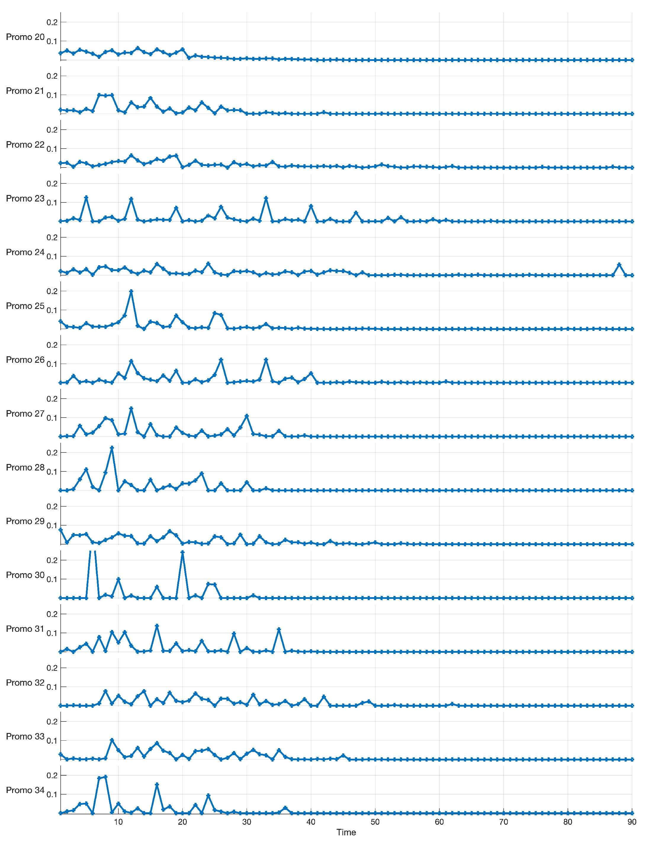
As an example of actual data, Figure 1 shows 15 out of 131 series related to the percentage sales enhancements over a horizon of 90 days (horizontal axis). Each series results from a specific promotion (named from “Promo 20” to “Promo 34”). Thus, the horizontal axis represents the sequence of days in three months, where the first day corresponds to the initial day of the promotion. It is worth noting that the observed sales series are not depending on the specific time data, and thus, the sales series are time-invariant. Alignment between sales series is obtained using the initial day of the promotion. The percentage enhancements of sales (vertical axis) are computed to the non-promotional (baseline) demand. In this case study, we are interested in investigating the effect of a promotion on the whole series of sales, starting from the initial day of the promotional campaign and for a time window of 90 days. This task is different from the common task of forecasting for a specific time index: it is related to clustering the whole time series into homogeneous groups. From Figure 1, we observe that “Promo 20”, “Promo 22”, and “Promo 23” induce relatively small variability, while the sales enhancements are not greater than . “Promo 28”, “Promo 30”, and “Promo 34” show higher variability, with sales enhancements equal or greater than and a different shape, which represents distinct impacts of the promotional campaign.
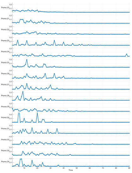
Figure 1.
Examples of time series related to the percentage sales enhancements over a horizon of 90 days (horizontal axis) of 15 promotional campaigns. The percentage sales enhancements (vertical axis) of the promotional demand is referred the non-promotional baseline demand.
There has been more attention in the recent literature to analyze sales with different promotional impacts and to find the most appropriate model in several conditions. A few empirical studies, which investigate the volatility of sales caused by promotion as a criterion to develop a forecasting model, are reported in [25,26]. In the present study, our interest is to present a method to partition the demand time series into homogeneous groups. The goal is to devise a statistical model that extracts knowledge from data for exploratory analysis.
2. Methodology
This section provides some necessary preliminaries about the methodology for finite mixture models for clustering. A detailed review of these methodologies can be found in [3]. The focus of the present study is on methods for exploratory analysis that rely on clustering techniques. Let , , be a random sample of n time series where is the response (e.g., the supply chain demand or the sales enhancements) for the ith individual given the time (predictor) t in time series. The time series of index is observed at the time values with for and .
2.1. The Finite Mixture Model for the Analysis of Time Series
A finite mixture model for time series assumes that the pairs are obtained from probability density components. is a discrete random variable, which indicates the component from which the pair is drawn. Thus, the following parametric density function describes a general finite mixture model.
where the parameter vector () is defined by
The coefficients are defined by , namely the mixing probabilities such that for each k and . is the dimension of . () is the vector of parameters for the kth component density. In finite mixture modeling, each of the component densities can be chosen to represent the time series for each group k; for example the regression mixture approaches [27], including spline and polynomial regression [28], as well as B-spline regression as in [29].
2.2. Maximization of Log-Likelihood
Consider a sample of n observed time series . The vector of parameters , in the finite mixture model in (1), can be estimated by maximizing the observed data log-likelihood, which is given by:
Maximization of this log-likelihood can not be performed in a closed-form. Instead, by the EM algorithm [5], we can obtain a consistent root of (3) by an iterative approach. The first step consists in considering the complete data log-likelihood by introducing the binary-valued variable . If the ith time series is obtained from the kth mixture component (), then , otherwise . The complete data log-likelihood is given by:
Starting with an initial solution , the EM algorithm alternates between two steps (E-step and M-step) summarized as follows.
E-step (update variables)
In this step, the algorithm calculates the expectation of the complete-data log-likelihood (4). Let be the current parameter vector. The expectation is equal to:
where
is the posterior probability of time series of index i, for component of index k.
M-step (update hypothesis)
This step updates the value of the parameter vector by maximizing the Q-function (5) with respect to
The updates of the mixing proportions are given by:
Both the E- and M-steps have simple forms when the data probability density function is a Gaussian probability density function.
2.3. Model-Based Time Series Clustering
After parameters estimation, a “soft” partition of the time series into K clusters, represented by the estimated posterior probabilities , is obtained. A “hard” partition is based on assigning each time series to the component having the highest estimated a posteriori probability defined by (6).
Determining the number of clusters K consists of selecting a compromise between flexibility and over-fitting by a criterion that measures this compromise. Therefore, an overall score function is formed of two terms. The first term measures the goodness of fit of the model to the data. It is represented by the log-likelihood . The second term measures the model complexity. It is characterized by the number of free parameters .
The most frequently used criteria for model selection are the well-known Bayesian Information Criterion (BIC) [30] and the Akaike Information Criterion (AIC) [31]. These criteria are penalized log-likelihood defined, respectively, by and . The log-likelihood is defined by (3) and the is given by the dimension of (2). A variant proposed in the literature is the Integrated Classification Likelihood (ICL) [32], which is defined by , with being the complete data log-likelihood for the model, as defined in (4).
4. Case Study
In our study, we collected real-world data from a food manufacturing company. Sales series data were available from the Point Of Sale (POS) systems, used to collect sales data for forecasting future demand. Modern POS systems provide a connected data gathering system for the retailer [34]. Sales data were aggregated across the retailers and spanned an observation period of 90 days.
The data set consists of 131 different time series of the percentage sales enhancements ranging between 0 (no sales enhancements) and 1 (highest sales enhancement). We computed sales enhancements (vertical axis) by adopting the non-promotional demand as the baseline. Each series refers to a specific combination promotion/product (labeled from “Promo 1” to “Promo 131”). The data set is included as a Supplementary Materials to the present paper. These series have different features influenced by the specific combination promotion/product. The above Figure 1 represents a subsample of 15 different time series out of the 131 in the dataset. Demand levels differ from each other, and these differences are mainly due to the promotion impact. The aim is to group time series into clusters, where the cluster labels are missing, and the number of clusters is unknown (a.k.a. unsupervised clustering).
In this section, we present the results of the algorithms previously described, concerning both B-spline and polynomial regression for auto-correlated time series clustering. The proposed approaches were coded in Matlab language using the R2021b version. The Matlab code ran on a 2.6 GHz Intel Core i7 with 16 Gb of memory. In terms of computing time, we observed that the algorithm was fast enough for both regression models. Although for large sample sizes and a large number of data series, the algorithms may lead to significant computational load, in the case study of the present paper, it converged after a few iterations requiring at most less than 240 s for 131 series data. This feature makes it useful for real practical situations.
4.1. B-Spline Regression Mixtures for Time Series Clustering
Table 1 reports the values of BIC for K ranging between 1 and 4 combined different spline orders. Generally, the most widely used orders for spline are 1, 2, and 4. For smooth function approximation, cubic B-splines, which correspond to order 4, are sufficient to approximate smooth functions. An order equal to 1 is selected for piecewise constant data. Spline knots were uniformly placed over the time series domain t.

Table 1.
BIC values for B-spline regression mixtures for different values of K and orders. The maximum BIC value is obtained for and order 4.
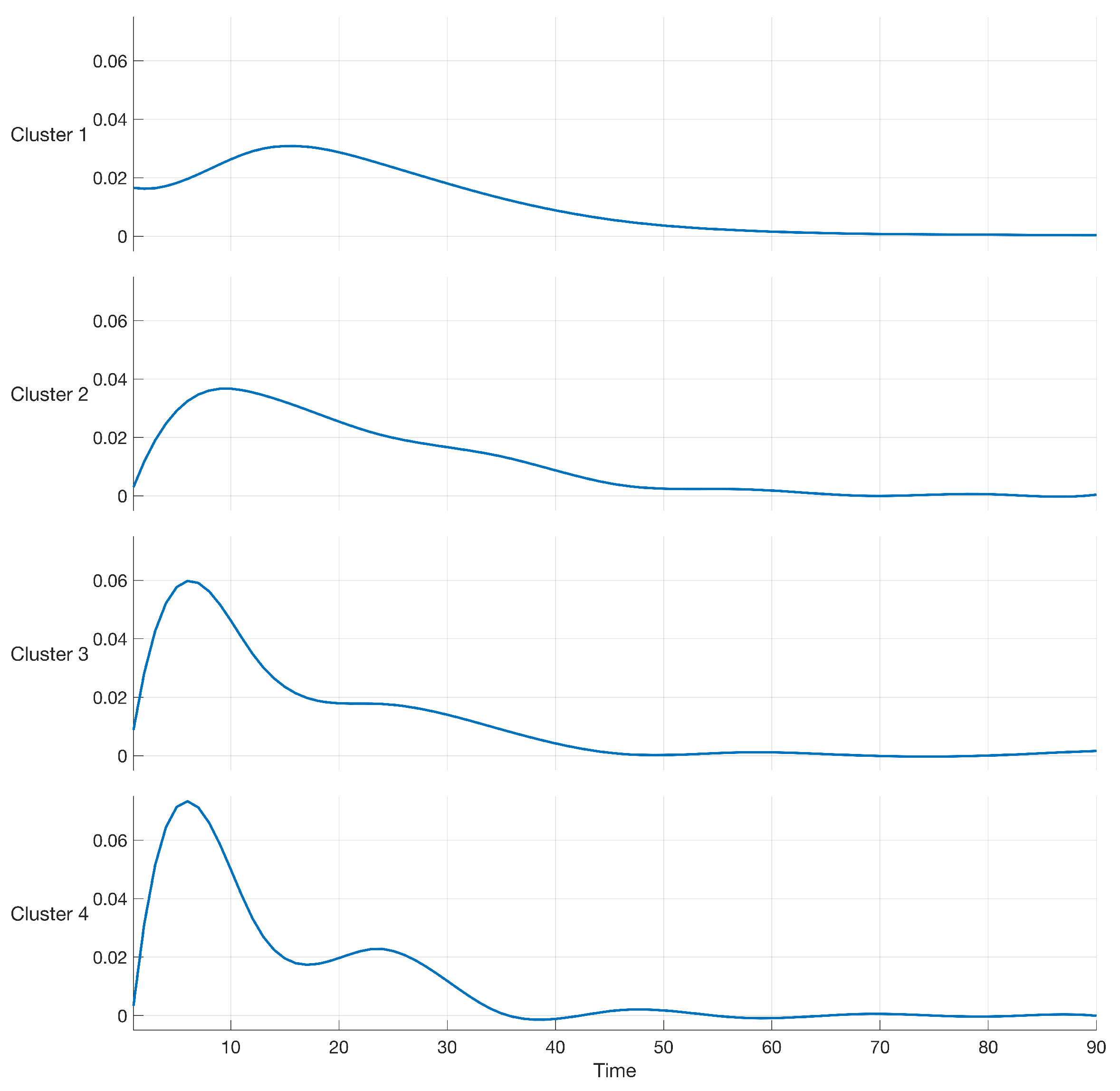
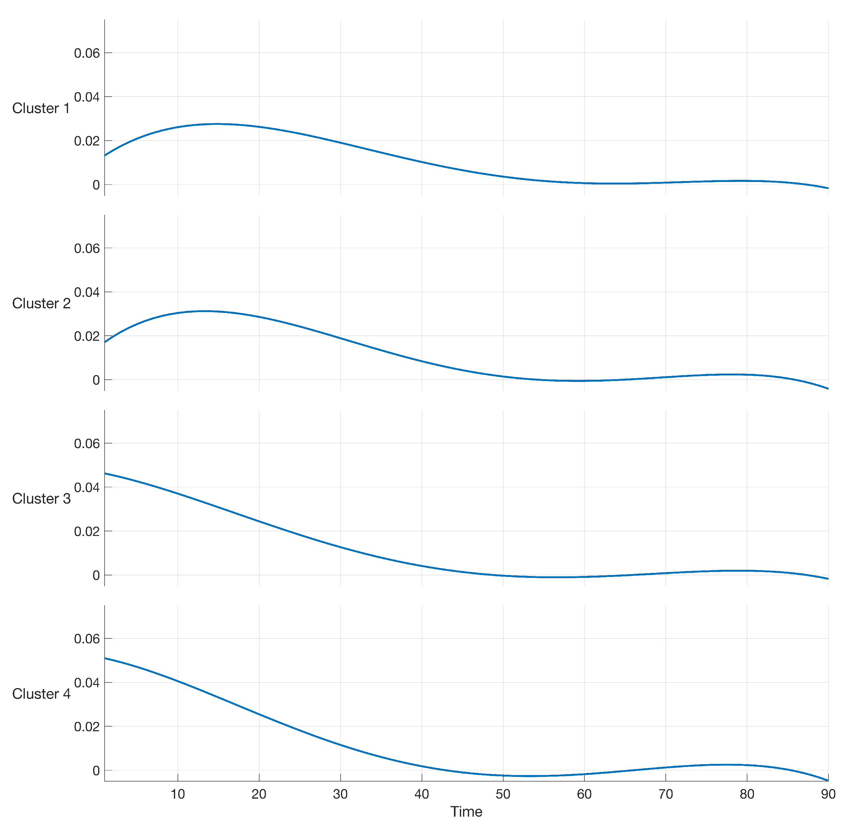
Results of Table 1 show that the maximum value of BIC, equal to 2.2029, was obtained by using a cubic B-spline of order 4 and a value of (number of clusters). The log-likelihood in (12) was maximized by using the APECM algorithm in Section 3. A graphical representation of the resulting cubic B-spline models of order 4 is reported in Figure 2.
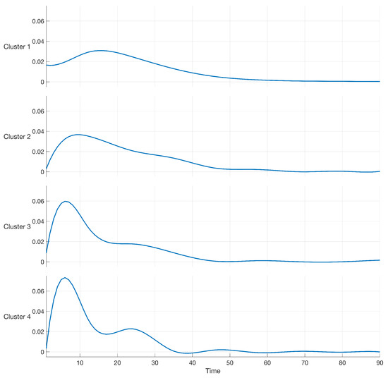
Figure 2.
Cubic B-spline of order 4 modeling the data in the case study.
From Figure 2, one can note that clusters numbers 1 and 2 present variabilities spanning more than 40 days, the shape of clusters numbers 3 and 4 present variabilities spanning a shorter period, with a higher peak in the first ten days. Figure 2 also shows that cluster number 4 presents two points of local maximization of sales during 90 days. Modeling the effect of promotions can contribute to knowing how the uncertainty of demand changes over time. This knowledge represents an essential source of information for the practitioner to optimize the upstream supply chain and avoid drawbacks such as the bullwhip effect and supply shortage [19,24].
Table 2 reports the final estimation values of , , and in (16) for each of the four clusters (components of the mixture model). In the case study, a maximum lag p equal to was considered adequate to model auto-correlation of data.
Table 2.
Sigma values and correlation factors of lag 1 and lag 2, for B-spline regression mixtures.
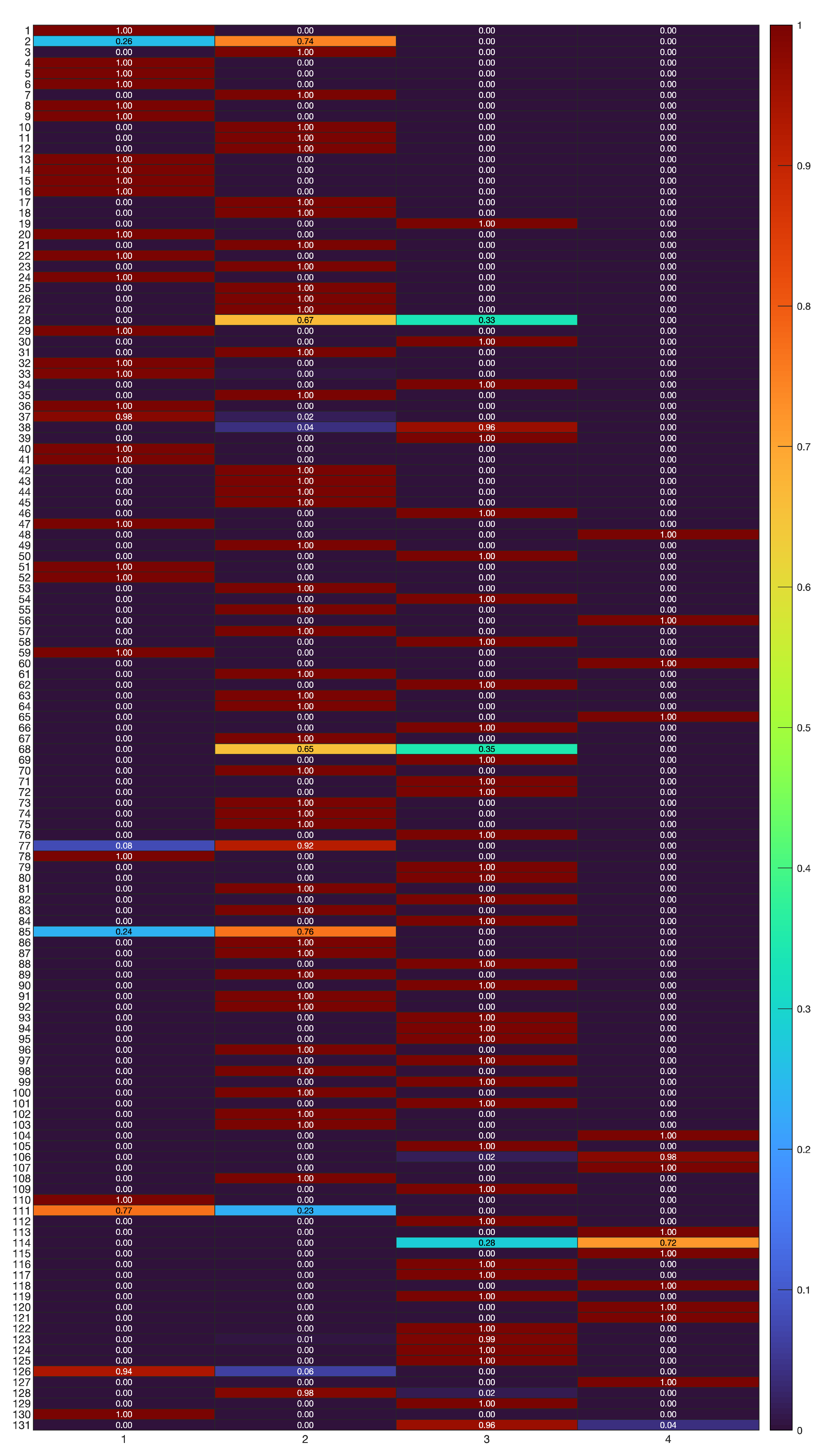
A “soft” partition of the time series into clusters, represented by the estimated posterior probabilities , is obtained as in (6). The values of are depicted in Figure 3, where a color scale (on the right) ranging between 0 and 1 is used to code the value of , for each time series out of the 131 in the case study, and for each cluster represented by the model depicted in previous Figure 2.
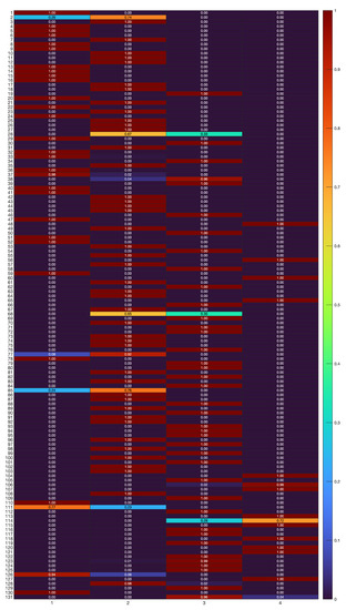
Figure 3.
Classification results with B-spline regression mixtures. “Soft” partition of the 131 time series (rows) into clusters (columns), represented by in (6).
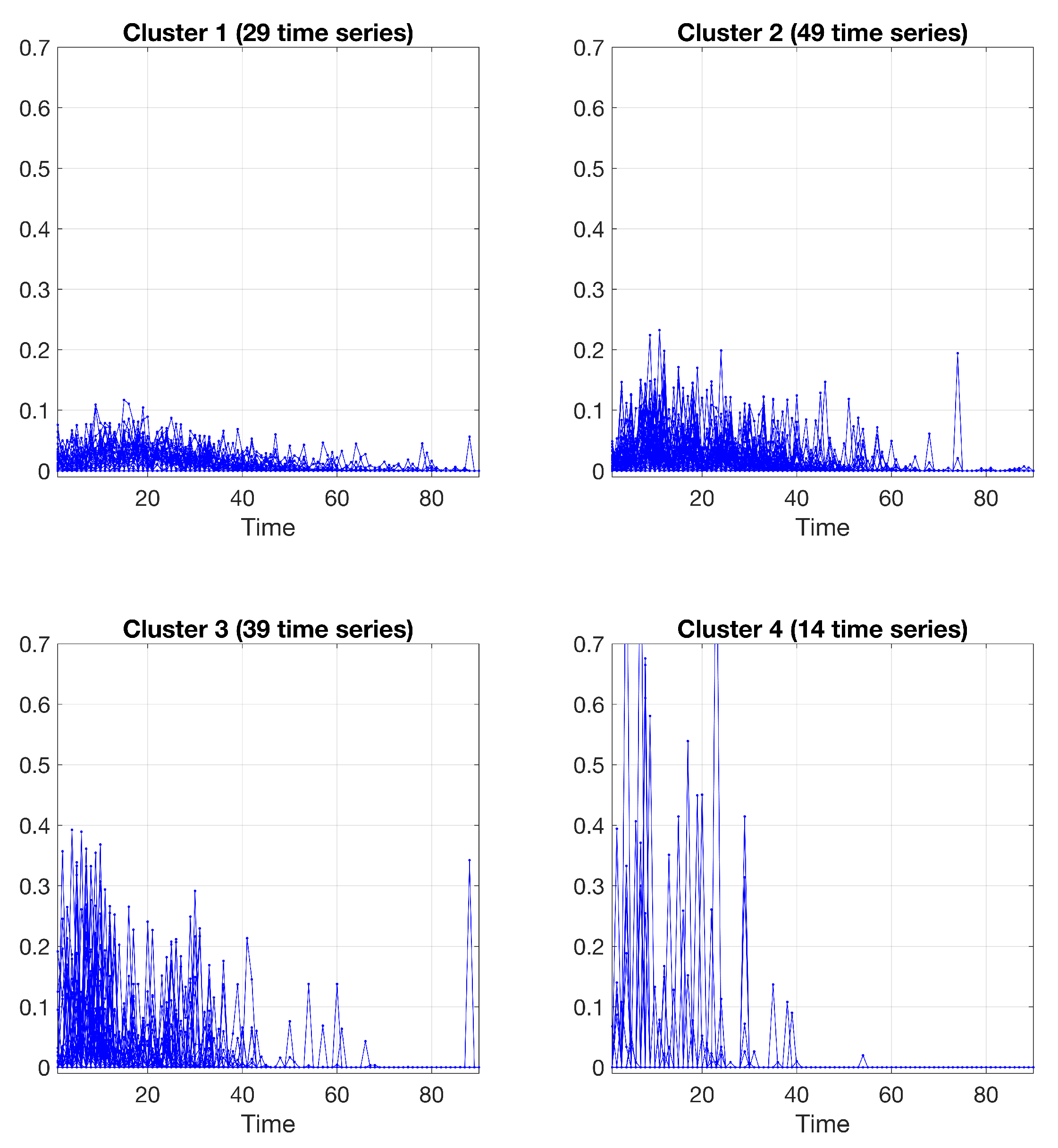
From the results in Figure 3, one can observe that the major uncertainties in clustering are limited to a few cases in the set of 131 time-series, specifically “Promo 2”, “Promo 28”, “Promo 68”, “Promo 85”, “Promo 111”, and “Promo 113”. A "hard" partition is obtained by allocating each time series to the component (cluster) having the most elevated posterior probability value . Figure 4 shows the final clustering of the time series data via the B-spline regression mixtures.

Figure 4.
Clustering results obtained by the spline regression model, using a cubic B-spline; 29 time series in cluster 1, 49 time series in cluster 2, 39 time series in cluster 3, and 14 time series in cluster 4.
4.2. Polynomial Regression Mixtures for Time Series Clustering
In this section, polynomial regression is used for time series clustering. Following Table 3, reports the value of the BIC for K ranging between 1 and 4. In Table 3, the BIC value is also reported for various polynomial orders.
Table 3.
BIC values for polynomial regression mixtures for different values of K and orders. The maximum BIC value is obtained for and order 4.
From the results in Table 3, we observe that the maximum value of BIC is 2.2027, and was obtained by using a polynomial of order 4 and a value of (number of clusters). Similar to the case of B-spline regression, the log-likelihood in (12) was maximized by using the EM algorithm. A graphical representation of the resulting polynomial models of order 4 is reported in the following Figure 5. Figure 5 clearly shows that, while clusters 1 and 2 present variabilities spanning more than 40 days, the shape of clusters 3 and 4 present variabilities spanning a shorter period, with higher values in the first 10 days. Table 4 reports the final estimation values of , , and in (16) for each of the four clusters (components of the mixture model).
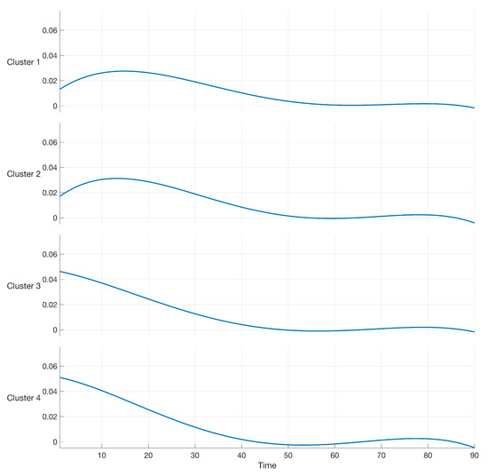
Figure 5.
Polynomial of order 4 modeling the data in the case study.
Table 4.
Sigma values and correlation factors of lag 1 and lag 2, for polynomial regression mixtures.
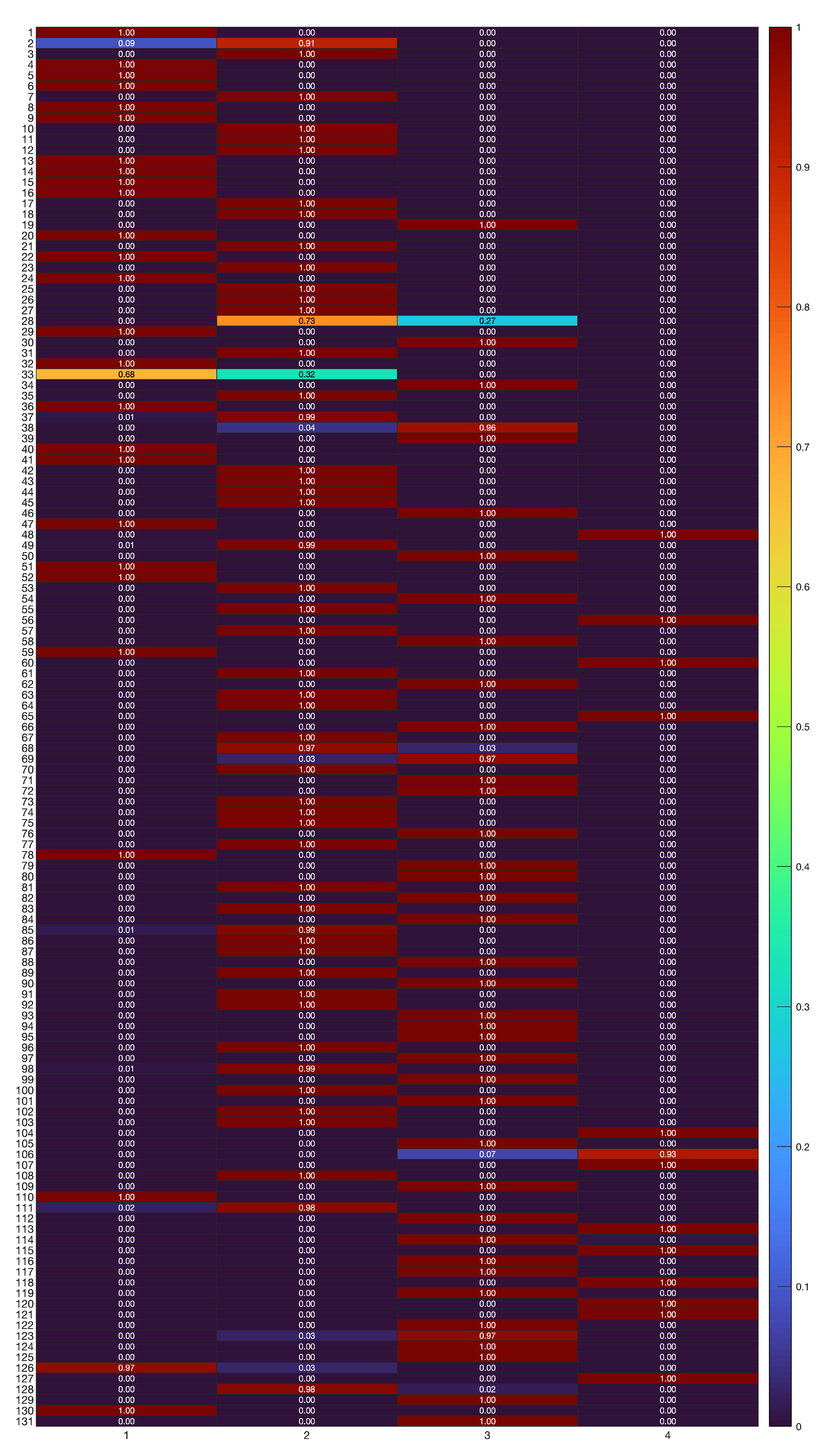
The values of related to the estimated posterior probabilities of the “soft” partition are represented in Figure 6. From the results in Figure 6, it can be noted that the uncertainties in clustering are limited to a fewer number of cases if compared to the B-spline results in previous Figure 3. Specifically, “Promo 2”, “Promo 28”, and “Promo 33”. Finally, a “hard” partition is obtained by allocating each time series to the component (cluster) having the most elevated posterior probability value . Figure 7 shows the clustering of the time series data via the polynomial regression mixtures.
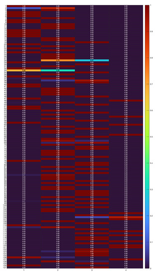
Figure 6.
Classification results with polynomial regression mixtures. “Soft” partition of the 131 time series (rows) into clusters (columns), represented by in (6).
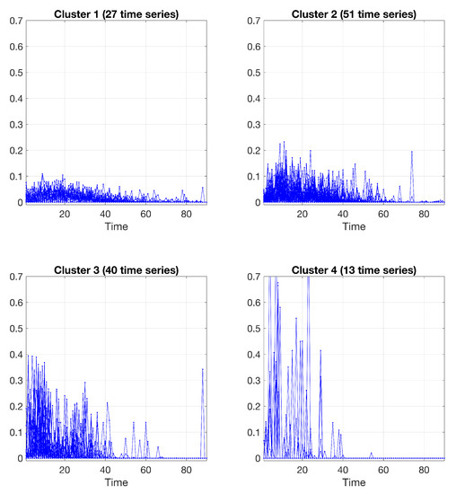
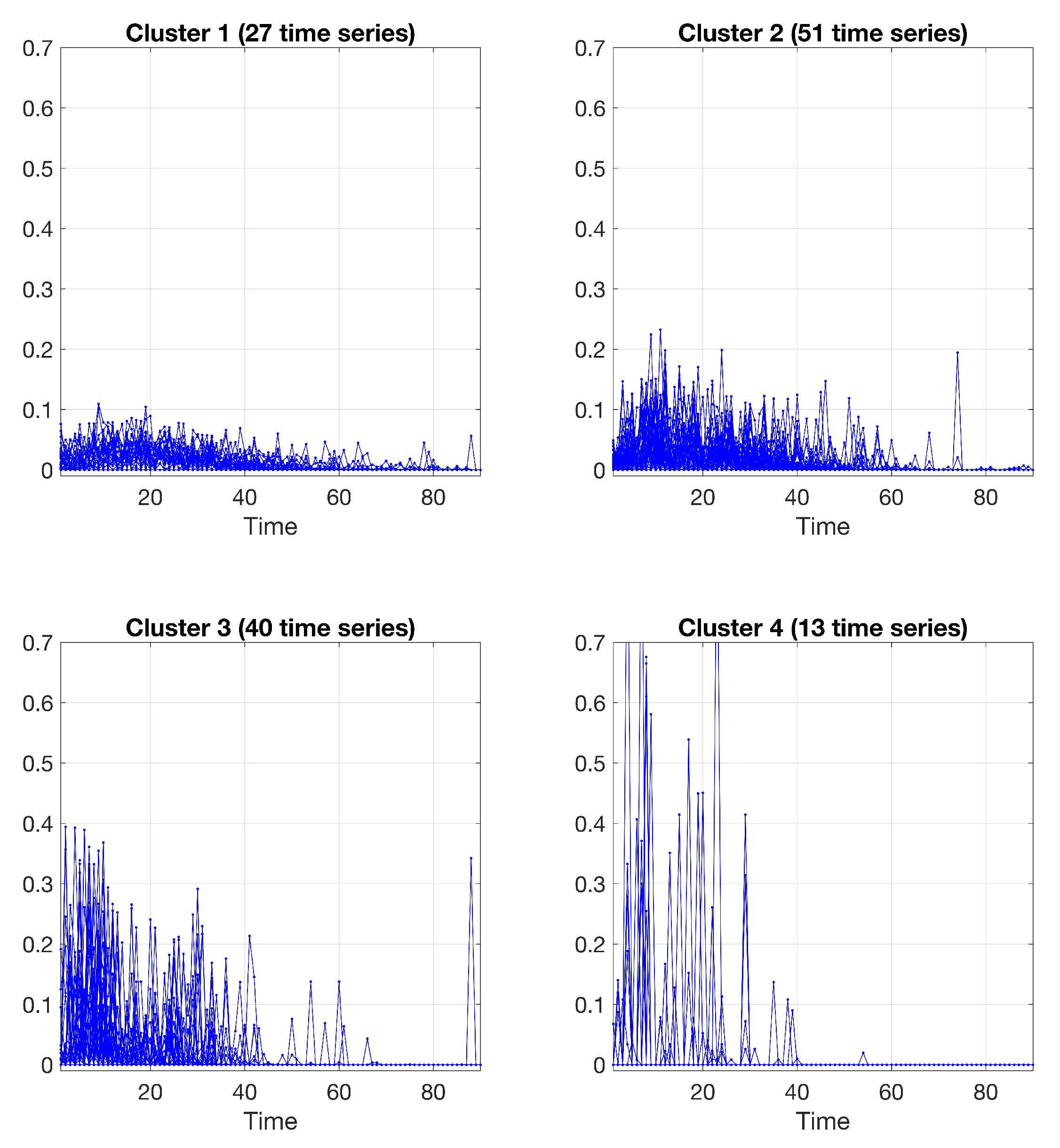
Figure 7.
Clustering results obtained by the polynomial regression model, using a polynomial of order 4; 27 time series in cluster 1, 51 time series in cluster 2, 40 time series in cluster 3, and 13 time series in cluster 4.
5. Conclusions
Modeling sales series data assume great importance for several managerial decisions at different levels of the supply chain. Promotion is one of the factors that can have differing effects on sales dynamics over the entire time series. Therefore, there is a need for a simple approach to model sales time series influenced by promotions as sophisticated models are useless in practice.
We analyzed the finite mixture models for time series clustering. The reason for using such models is their sound statistical basis and the interpretability of their results. The fitted values for their posterior membership probabilities provide the uncertainties that the data belong to clusters. Moreover, as clusters correspond to model components, choosing the number of them can be easily implemented in terms of the likelihood function for the components in the mixture model.
We developed an approach for clustering auto-correlated time series. In particular, we implemented the APECM algorithm combined with spline and polynomial regression through autoregressive mixtures as a novel model-based clustering algorithm for auto-correlated times series.
We demonstrated the capabilities of the developed approach for dealing with time-series data with several complex data situations, including heterogeneity and dynamical behavior. We explored two regression mixtures approaches by implementing both B-spline and polynomial models. Numerical results on 131 real-world time series data demonstrate the advantage of the mixture model-based approach presented in this study for time series clustering. For the data set used in this study, the spline and polynomial order with the best BIC value were considered. For the spline regression mixtures, we used cubic B-splines because cubic splines, which correspond to a spline of order 4, are sufficient to approximate smooth functions. For the polynomial regression mixtures, we observed that an order 4 was satisfactory for the dataset of the case study. The results from the case study demonstrate the efficacy of the proposed method for clustering auto-correlated time series. Despite the specific case study of this paper, our approach can be used in different real-world application fields.
The most important benefit of the research presented in this paper is the parametric model-based approach. A model-based approach is a convenient, understandable description, allowing the analyst to access and interpret each component of the real-world systems. The main drawback of this approach is related to the fact that the user should be able to select the most appropriate structure of the model, selecting the type of regressors (spline and polynomial), the order of the regressors, the number of clusters, and the order of the autoregressive component. In our approach, we used a BIC-based rule for model selection. The main limitation of this approach is the computational requirements caused by dealing with large datasets, as in the framework of Big Data. In these cases, a data-driven method for time series clustering/classification, such as deep learning approaches, should be considered instead [35,36].
Supplementary Materials
The following supporting information can be downloaded at: https://www.mdpi.com/article/10.3390/computation10020023/s1.
Author Contributions
Conceptualization, M.P.; methodology, M.P.; software, M.P.; validation, M.P. and G.P.; resources, G.P.; writing—original draft preparation, M.P.; writing—review and editing, M.P. and G.P.; supervision, G.P.; project administration, G.P.; and funding acquisition, G.P. All authors have read and agreed to the published version of the manuscript.
Funding
This work has been funded by Puglia Region (Italy)—Project ‘Cooperative Supply Chain’.
Institutional Review Board Statement
Not applicable.
Informed Consent Statement
Not applicable.
Data Availability Statement
The data set of the case study is included as a Supplementary Materials to the present paper.
Acknowledgments
The authors are thankful to DGS S.p.A. (Italy) for providing the data set of the case study.
Conflicts of Interest
The authors declare no conflict of interest. The funder had no role in the design of the study; in the collection, analyses, or interpretation of data; in the writing of the manuscript, or in the decision to publish the results.
References
- Aghabozorgi, S.; Shirkhorshidi, A.S.; Wah, T.Y. Time-series clustering—A decade review. Inf. Syst. 2015, 53, 16–38. [Google Scholar] [CrossRef]
- Javed, A.; Lee, B.S.; Rizzo, D.M. A benchmark study on time series clustering. Mach. Learn. Appl. 2020, 1, 100001. [Google Scholar] [CrossRef]
- Fraley, C.; Raftery, A.E. Model-based clustering, discriminant analysis, and density estimation. J. Am. Stat. Assoc. 2002, 97, 611–631. [Google Scholar] [CrossRef]
- Chen, W.C.; Maitra, R. Model-based clustering of regression time series data via APECM—An AECM algorithm sung to an even faster beat. Stat. Anal. Data Min. ASA Data Sci. J. 2011, 4, 567–578. [Google Scholar] [CrossRef]
- Dempster, A.P.; Laird, N.M.; Rubin, D.B. Maximum Likelihood from Incomplete Data Via the EM Algorithm. J. R. Stat. Soc. Ser. B 1977, 39, 1–22. [Google Scholar]
- Chen, W.C.; Ostrouchov, G.; Pugmire, D.; Prabhat; Wehner, M. A parallel EM algorithm for model-based clustering applied to the exploration of large spatio-temporal data. Technometrics 2013, 55, 513–523. [Google Scholar] [CrossRef]
- Michael, S.; Melnykov, V. Finite mixture modeling of Gaussian regression time series with application to dendrochronology. J. Classif. 2016, 33, 412–441. [Google Scholar] [CrossRef]
- Narayanan, A.; Sahin, F.; Robinson, E.P. Demand and order-fulfillment planning: The impact of point-of-sale data, retailer orders and distribution center orders on forecast accuracy. J. Oper. Manag. 2019, 65, 468–486. [Google Scholar] [CrossRef]
- Silver, E.A.; Pyke, D.F.; Peterson, R. Inventory Management and Production Planning and Scheduling; Wiley: New York, NY, USA, 1998; Volume 3. [Google Scholar]
- Donohue, K.L. Efficient supply contracts for fashion goods with forecast updating and two production modes. Manag. Sci. 2000, 46, 1397–1411. [Google Scholar] [CrossRef]
- Hyndman, R.J.; Athanasopoulos, G. Forecasting: Principles and Practice, 2nd ed.; OTexts: Melbourne, Australia, 2018. [Google Scholar]
- Aye, G.C.; Balcilar, M.; Gupta, R.; Majumdar, A. Forecasting aggregate retail sales: The case of South Africa. Int. J. Prod. Econ. 2015, 160, 66–79. [Google Scholar] [CrossRef] [Green Version]
- Syntetos, A.A.; Babai, Z.; Boylan, J.E.; Kolassa, S.; Nikolopoulos, K. Supply chain forecasting: Theory, practice, their gap and the future. Eur. J. Oper. Res. 2016, 252, 1–26. [Google Scholar] [CrossRef]
- Pacella, M.; Papadia, G. Evaluation of deep learning with long short-term memory networks for time series forecasting in supply chain management. Procedia CIRP 2021, 99, 604–609. [Google Scholar] [CrossRef]
- Jung, H.; Jeong, S.J. Managing demand uncertainty through fuzzy inference in supply chain planning. Int. J. Prod. Res. 2012, 50, 5415–5429. [Google Scholar] [CrossRef]
- Chopra, S.; Meindl, P.; Kalra, D.V. Supply Chain Management: Strategy, Planning, and Operation; Pearson: Boston, MA, USA, 2013; Volume 232. [Google Scholar]
- Chen, F.; Drezner, Z.; Ryan, J.K.; Simchi-Levi, D. Quantifying the bullwhip effect in a simple supply chain: The impact of forecasting, lead times, and information. Manag. Sci. 2000, 46, 436–443. [Google Scholar] [CrossRef] [Green Version]
- Zhang, X. The impact of forecasting methods on the bullwhip effect. Int. J. Prod. Econ. 2004, 88, 15–27. [Google Scholar] [CrossRef]
- Packowski, J. LEAN Supply Chain Planning: The New Supply Chain Management Paradigm for Process Industries to Master Today’s VUCA World; CRC Press: Boca Raton, FL, USA, 2013. [Google Scholar]
- Nikolopoulos, K.; Litsa, A.; Petropoulos, F.; Bougioukos, V.; Khammash, M. Relative performance of methods for forecasting special events. J. Bus. Res. 2015, 68, 1785–1791. [Google Scholar] [CrossRef] [Green Version]
- Ramanathan, U.; Muyldermans, L. Identifying the underlying structure of demand during promotions: A structural equation modelling approach. Expert Syst. Appl. 2011, 38, 5544–5552. [Google Scholar] [CrossRef]
- Ramanathan, U. Supply chain collaboration for improved forecast accuracy of promotional sales. Int. J. Oper. Prod. Manag. 2012, 32, 676–695. [Google Scholar] [CrossRef]
- Blattberg, R.C.; Neslin, S.A. Sales promotion models. Handbooks Oper. Res. Manag. Sci. 1993, 5, 553–609. [Google Scholar]
- Cachon, G.P. Managing supply chain demand variability with scheduled ordering policies. Manag. Sci. 1999, 45, 843–856. [Google Scholar] [CrossRef] [Green Version]
- Abolghasemi, M.; Beh, E.; Tarr, G.; Gerlach, R. Demand forecasting in supply chain: The impact of demand volatility in the presence of promotion. Comput. Ind. Eng. 2020, 142, 106380. [Google Scholar] [CrossRef] [Green Version]
- Abolghasemi, M.; Hurley, J.; Eshragh, A.; Fahimnia, B. Demand forecasting in the presence of systematic events: Cases in capturing sales promotions. Int. J. Prod. Econ. 2020, 230, 107892. [Google Scholar] [CrossRef]
- Gaffney, S.; Smyth, P. Curve Clustering with Random Effects Regression Mixtures. In Proceedings of the Ninth International Workshop on Artificial Intelligence and Statistics, Key West, FL, USA, 3–6 January 2003; Volume R4, pp. 101–108. [Google Scholar]
- James, G.M.; Sugar, C.A. Clustering for Sparsely Sampled Functional Data. J. Am. Stat. Assoc. 2003, 98, 397–408. [Google Scholar] [CrossRef]
- Liu, X.; Yang, M.C. Simultaneous curve registration and clustering for functional data. Comput. Stat. Data Anal. 2009, 53, 1361–1376. [Google Scholar] [CrossRef]
- Schwarz, G. Estimating the Dimension of a Model. Ann. Stat. 1978, 6, 461–464. [Google Scholar] [CrossRef]
- Akaike, H. A new look at the statistical model identification. IEEE Trans. Autom. Control 1974, 19, 716–723. [Google Scholar] [CrossRef]
- Biernacki, C.; Celeux, G.; Govaert, G. Assessing a mixture model for clustering with the integrated completed likelihood. IEEE Trans. Pattern Anal. Mach. Intell. 2000, 22, 719–725. [Google Scholar] [CrossRef]
- Chamroukhi, F. Unsupervised learning of regression mixture models with unknown number of components. J. Stat. Comput. Simul. 2016, 86, 2308–2334. [Google Scholar] [CrossRef] [Green Version]
- Boone, T.; Ganeshan, R.; Jain, A.; Sanders, N.R. Forecasting sales in the supply chain: Consumer analytics in the big data era. Int. J. Forecast. 2019, 35, 170–180. [Google Scholar] [CrossRef]
- Pacella, M. Unsupervised classification of multichannel profile data using PCA: An application to an emission control system. Comput. Ind. Eng. 2018, 122, 161–169. [Google Scholar] [CrossRef]
- Fawaz, H.I.; Forestier, G.; Weber, J.; Idoumghar, L.; Muller, P.A. Deep learning for time series classification: A review. Data Min. Knowl. Discov. 2019, 33, 917–963. [Google Scholar] [CrossRef] [Green Version]
Publisher’s Note: MDPI stays neutral with regard to jurisdictional claims in published maps and institutional affiliations. |
© 2022 by the authors. Licensee MDPI, Basel, Switzerland. This article is an open access article distributed under the terms and conditions of the Creative Commons Attribution (CC BY) license (https://creativecommons.org/licenses/by/4.0/).