Bayesian Instability of Optical Imaging: Ill Conditioning of Inverse Linear and Nonlinear Radiative Transfer Equation in the Fluid Regime

Abstract

For the inverse problem in physical models, one measures the solution and infers the model parameters using information from the collected data. Oftentimes, these data are inadequate and render the inverse problem ill-posed. We study the ill-posedness in the context of optical imaging, which is a medical imaging technique that uses light to probe (bio-)tissue structure. Depending on the intensity of the light, the forward problem can be described by different types of equations. High-energy light scatters very little, and one uses the radiative transfer equation (RTE) as the model; low-energy light scatters frequently, so the diffusion equation (DE) suffices to be a good approximation. A multiscale approximation links the hyperbolic-type RTE with the parabolic-type DE. The inverse problems for the two equations have a multiscale passage as well, so one expects that as the energy of the photons diminishes, the inverse problem changes from well- to ill-posed. We study this stability deterioration using the Bayesian inference. In particular, we use the Kullback–Leibler divergence between the prior distribution and the posterior distribution based on the RTE to prove that the information gain from the measurement vanishes as the energy of the photons decreases, so that the inverse problem is ill-posed in the diffusive regime. In the linearized setting, we also show that the mean square error of the posterior distribution increases as we approach the diffusive regime.

1. Introduction

Optical tomography is a well-defined inverse problem. In the lab, laser beams with high-energy photons are injected into bio-tissues to detect the interior optical property [1]. This helps identify unhealthy bio-tissues for treatment. Mathematically, this amounts to reconstructing the optical coefficients, such as the scattering and the absorption coefficients in the radiative transfer equation (RTE), which is a model equation that describes the propagation of photon particles [2]. The equation, in its simplest form, reads

$${\partial }_{t}f+\frac{1}{ϵ}v·{\nabla }_{x}f=\frac{1}{{ϵ}^2}\mathcal{Q}\left[f\right].$$

(1)

The unknown $f(t,x,v)$ describes the number of photon particles at time $t\in {\mathbb{R}}^{+}$, location $x\in \mathsf{\Omega }\subseteq {\mathbb{R}}^d$, and traveling with velocity $v\in {\mathbb{S}}^{d-1}$. The dimension of the problem is $d=2,3$. v is the travel direction of the particles and therefore belongs to a unit ball. The two terms in the equation represent the transport and the scattering effect, respectively. The transport term characterizes $\dot{x}=v$, while the scattering term $\mathcal{Q}\left[f\right]$ describes the way the photon particles interact with the media. When the temperature is fixed, this operator is a linear operator, whereas if the laser beam heats up the tissue, $\mathcal{Q}$ reflects the nonlinear dependence on the temperature. This is the term that encodes the optical property of the media.

In the steady state, the ${\partial }_{t}f$ term is dropped, and the equation balances the transport term and the scattering term. The equation is well-posed if equipped with Dirichlet-type boundary condition [3,4,5,6]:

$${f|}_{{\mathsf{\Gamma }}_{-}}=\varphi ,$$

(2)

where ${\mathsf{\Gamma }}_{\pm }$ collects the coordinates on the physical boundary $\partial \mathsf{\Omega }$ with the velocity either pointing in or out of the domain:

$${\mathsf{\Gamma }}_{\pm }=\{(x,v):x\in \partial \mathsf{\Omega },\pm v·n_x>0\}={\cup }_{x\in \partial \mathsf{\Omega }}{\mathsf{\Gamma }}_{\pm }\left(x\right),\mathrm{where}{\mathsf{\Gamma }}_{\pm }\left(x\right)=\{v:\pm v·n_x>0\}.$$

In practice, the laser light is shined into the domain, meaning that $\varphi$ is prescribed. Then, one detects the number of photons scattered out of the domain by measuring ${f|}_{{\mathsf{\Gamma }}_{+}}$. We term this operator the albedo operator:

$${\mathcal{A}}_{\mathcal{Q}}:f{{|}_{{\mathsf{\Gamma }}_{-}}\to f|}_{{\mathsf{\Gamma }}_{+}},$$

where the subindex $\mathcal{Q}$ reflects the influence of $\mathcal{Q}$. Therefore, optical tomography amounts to reconstructing the coefficients in $\mathcal{Q}$ using the information in the operator ${\mathcal{A}}_{\mathcal{Q}}$. The general well-posedness theory of such an inverse problem was addressed in the pioneering papers [7,8]. The result on the stability was established in [9,10,11], and see [12] for a review.

One key parameter in Equation (1) is $ϵ$, which is the Knudsen number. It describes the regime the system is in. By definition, the Knudsen number is the ratio of the mean-free path and the domain length. Physically, if a photon has low energy (visible or near-infrared light), it travels only a short distance before being scattered, and the mean-free path is short compared to the domain length, leading to a small $ϵ$. When this happens, one typically observes a diffused light phenomenon, and the received images are blurred. The situation is termed the diffusion effect, and in this regime, RTE, either linear or nonlinear, can be asymptotically approximated by a diffusive equation that characterizes macroscopic quantities such as the density $\rho \left(x\right)=\int f(x,v)\mathrm{d}v$. Depending on the form of $\mathcal{Q}$, this limiting equation for $\rho$ is accordingly adjusted. Details regarding the diffusion limit can be found in [13,14].

Intuitively, as one decreases the photon energy, the received picture loses its crisp, and the reconstruction becomes more unstable. The perturbation observed in the measurement is enlarged in the reconstructed coefficients. This phenomenon has been been numerically observed in [1,15,16] and proved rigorously in [17], in which the authors investigate the stability deterioration of the inverse problem as $ϵ\to 0$. However, all these results heavily depend on the theoretical framework where it is assumed that one has the access to the full map$\mathcal{A}$. This amounts to sending in all kinds of incoming data $\varphi$ and taking the measurement over the entire ${\mathsf{\Gamma }}_{+}$.

These theoretical results are helpful in building the foundation for understanding the stability deterioration, but the setup is infeasible numerically or practically. In the lab, a finite number of incoming configurations can be taken, and the detectors can measure outgoing photons in a finite number of locations. Therefore, new theory needs to be developed to account for this real situation [18,19]. To put the problem in a mathematical framework, we denote ${\left\{{\varphi }_j\right\}}_{j=1}^J$ as the incoming data and ${\left\{x_k\right\}}_{k=1}^K$ as the location of the detectors; then, the measurements are

$$\mathcal{G}={\left\{{\mathcal{G}}_{jk}\right\}}_{j=1,k=1}^{J,K},\mathrm{with}{\mathcal{G}}_{jk}={\int }_{v\in {\mathsf{\Gamma }}_{+}\left(x_k\right)}{\mathcal{A}}_{\mathcal{Q}}\left[{\varphi }_j\right]|v·n_{x_k}|\mathrm{d}v.$$

Equivalently, denoting $f_j$ as the solution to (1) with the boundary condition in (2) being ${\varphi }_j$, then:

$${\mathcal{G}}_{jk}={\int }_{v\in {\mathsf{\Gamma }}_{+}\left(x_k\right)}{f}_j(x_k,v)|v·n_{x_k}|\mathrm{d}v.$$

With the finite amount of data points, to find the coefficients in $\mathcal{Q}$, one can either adopt the PDE-constrained minimization algorithms [20,21,22] or employ the Bayesian inference [23,24,25]. While this finite setting greatly affects the well-posedness argument [26,27,28], the physical intuition still holds true in the sense that the reconstruction is expected to become more and more unstable as $ϵ$ diminishes.

In this paper, we quantify the stability deterioration in the Bayesian inference framework with a finite number of data points. To quantify “stability”, we propose two measures: one is a global measure that evaluates the information gain by comparing the posterior and prior distributions, and the other is a local measure that characterizes the “flatness” of the posterior distribution around the MAP (maximum a posteriori) point. More particularly, at the global level, we measure the difference between the posterior and prior distributions using the KL (Kullback–Leibler) divergence. Since the posterior distribution of the coefficients takes both the prior knowledge and the measured data into account, this divergence essentially characterizes by how much the data are driving the final guess away from the prior guess. At the local level, we estimate the Hessian of the posterior distribution around the MAP point, which essentially describes the uncertainty level of the optimizer. For both measures, we analyze their dependence on $ϵ$, and we reveal the stability relation between two regimes, the transport regime and diffusive regime, in a more rigorous way. We will present our theory through the lens of both linear and nonlinear RTEs, but we shall mention that other multiscale kinetic models may have such a relation in the inverse setting; see for instance in [29,30,31].

The rest of the paper is organized as follows. In the next section, we recall some formulation in the Bayesian inference problem and demonstrate a general relation in the KL divergence between prior and posterior distribution, through which we will address the stability deterioration from the global point of view. In Section 3, we consider the inverse problem for the linear radiative transfer equation, and we show that the KL divergence is of order $ϵ$, which diminishes as we approach the diffusive regime. We extend the investigation to the nonlinear RTE in Section 4 and obtain similar results. In Section 5, we focus on the local viewpoint by estimating the second derivative of the parameter-to-measurement map, and we show that it decreases at the order of $ϵ$, indicating that the posterior distribution becomes flatter near the diffusive regime and therefore is less sensitive to the measurement data, rendering the inverse problem more unstable. We summarize our theoretical results and provide some numerical evidence in Section 6. A final conclusion of the paper is drawn in Section 7.

All the discussion in these sections finally achieve the following aim of the paper: to demonstrate, in the Bayesian inference framework, the stability deterioration of optical imaging when the impinging light uses low-energy photons.

2. Bayesian Formulation Basics

Bayesian inference is one of the most popular numerical methods for inferring unknown parameters. In this section, we give a quick overview of definitions to be used in this paper.

To start, we define the parameter to measurement map $\mathcal{G}:{\mathcal{B}}_{\sigma }\mapsto {\mathbb{R}}^q$ and denote $\eta$ the measurement error:

$$d=\mathcal{G}\left(\sigma \right)+\eta ,$$

where the measurement $d\in {\mathbb{R}}^q$, the measurement error $\eta \in {\mathbb{R}}^d$, and $\sigma \in B\subset {\mathcal{B}}_{\sigma }$, the admissible set in a pre-defined Banach space ${\mathcal{B}}_{\sigma }$:

$$B=\{\sigma \in {\mathcal{B}}_{\sigma }:\parallel \mathcal{G}\left(\sigma \right){\parallel }_{L_{\infty }\left(\mathsf{\Omega }\right)}<C_B\}.$$

(3)

Note that ${\mathcal{B}}_{\sigma }$ can be a function space specified in (10), and $\sigma$ is a function in this space. Throughout the paper, we assume that $\eta$ is an additive noise generated by a Gaussian distribution $\mathcal{N}(0,{\mathsf{\Gamma }}_{\eta })$, and ${\mathsf{\Gamma }}_{\eta }$ is a $q\times q$ dimensional matrix.

In Bayesian inference, one needs to prepare a prior distribution for $\sigma$. Denote $\mathcal{F}$ as the $\sigma$-algebra of B and ${\mu }_0$ as the prior probability measure on B. According to the Bayes’ rule, the posterior distribution ${\mu }_{\mathrm{post}}=\mu \left(\sigma \right|d)$ is given according to its Radon–Nikodym derivative with respect to $d{\mu }_0$:

$$\frac{\mathrm{d}{\mu }_{\mathrm{post}}}{\mathrm{d}{\mu }_0}\propto \frac{1}{Z}exp\left(-\frac{1}{2}{\parallel \mathcal{G}\left(\sigma \right)-d\parallel }_{{\mathsf{\Gamma }}_{\eta }}^2\right),$$

(4)

where Z is the normalization constant:

$$Z={\int }_{B}exp\left(-\frac{1}{2}{\parallel \mathcal{G}\left(\sigma \right)-d\parallel }_{{\mathsf{\Gamma }}_{\eta }}^2\right)\mathrm{d}{\mu }_0\left(\sigma \right),$$

and the mismatch is weighted by ${\mathsf{\Gamma }}_{\eta }$

$${\parallel \mathcal{G}\left(\sigma \right)-d\parallel }_{{\mathsf{\Gamma }}_{\eta }}^2={(\mathcal{G}\left(\sigma \right)-d)}^T{\mathsf{\Gamma }}_{\eta }^{-1}(\mathcal{G}\left(\sigma \right)-d).$$

Suppose ${\mu }_{1,2}$ are two distinct probability measures; then, the KL divergence measures the distance between them:

$$D_{\mathrm{KL}}\left({\mu }_1\right|{\mu }_2)={\int }_{\mathcal{X}}log\left(\frac{\mathrm{d}{\mu }_1}{\mathrm{d}{\mu }_2}\right)\mathrm{d}{\mu }_1.$$

when this definition is used in Bayesian inference to quantify the relative gain through the measurement process, one defines the relative entropy, and in the particular setting of (4), we have the following proposition.

Proposition 1.

Assume $\sigma \in B$; then, the KL divergence between ${\mu }_{\mathit{post}}$ and ${\mu }_0$ has the following estimate:

$${\mathrm{D}}_{KL}\left({\mu }_0\right|{\mu }_{\mathit{post}})\le C{\int }_B{\int }_B\left|(\mathcal{G}\left({\sigma }^{\prime }\right)-\mathcal{G}\left(\sigma \right)){\mathsf{\Gamma }}_{\eta }^{-1}(\mathcal{G}\left(\sigma \right)+\mathcal{G}\left({\sigma }^{\prime }\right)-2d)\right|\mathrm{d}{\mu }_0\left({\sigma }^{\prime }\right)\mathrm{d}{\mu }_0\left(\sigma \right)$$

(5)

for some positive constant C independent of B.

Proof. 

Since ${\mu }_0$ and ${\mu }_{\mathrm{post}}$ are mutually absolutely continuous, according to (4), we have

$$\begin{array}{cc}\hfill {\mathrm{D}}_{KL}\left({\mu }_0\right|{\mu }_{\mathrm{post}})& ={\int }_{B}log\left(\frac{\mathrm{d}{\mu }_0}{\mathrm{d}{\mu }_{\mathrm{post}}}\right)\mathrm{d}{\mu }_0\hfill \\ & ={\int }_B\left(\frac{1}{2}{\parallel \mathcal{G}\left(\sigma \right)-d\parallel }_{{\mathsf{\Gamma }}_{\eta }}^2+logZ\right)\mathrm{d}{\mu }_0.\hfill \end{array}$$

Denoting $\mathcal{B}\left(\sigma \right)=\frac{1}{2}{\parallel \mathcal{G}\left(\sigma \right)-d\parallel }_{{\mathsf{\Gamma }}_{\eta }}^2$, we proceed with:

$$\begin{array}{cc}\hfill {\mathrm{D}}_{KL}\left({\mu }_0\right|{\mu }_{\mathrm{post}})& ={\int }_B\left[\mathcal{B}\left(\sigma \right)+log\left({\int }_B{e}^{-\mathcal{B}\left({\sigma }^{\prime }\right)}\mathrm{d}{\mu }_0\left({\sigma }^{\prime }\right)\right)\right]\mathrm{d}{\mu }_0\left(\sigma \right)\hfill \\ & ={\int }_B\left[-log{e}^{-\mathcal{B}\left(\sigma \right)}+log\left({\int }_B{e}^{-\mathcal{B}\left({\sigma }^{\prime }\right)}\mathrm{d}{\mu }_0\left({\sigma }^{\prime }\right)\right)\right]\mathrm{d}{\mu }_0\left(\sigma \right)\hfill \\ & \le C{\int }_B\left[-e^{-\mathcal{B}\left(\sigma \right)}+\left({\int }_B{e}^{-\mathcal{B}\left({\sigma }^{\prime }\right)}\mathrm{d}{\mu }_0\left({\sigma }^{\prime }\right)\right)\right]\mathrm{d}{\mu }_0\left(\sigma \right)\hfill \\ & \le C{\int }_B{\int }_B|e^{-\mathcal{B}\left(\sigma \right)}-e^{-\mathcal{B}\left({\sigma }^{\prime }\right)}|\mathrm{d}{\mu }_0\left({\sigma }^{\prime }\right)\mathrm{d}{\mu }_0\left(\sigma \right)\hfill \\ & \le C{\int }_B{\int }_B|\mathcal{B}\left(\sigma \right)-\mathcal{B}\left({\sigma }^{\prime }\right)|\mathrm{d}{\mu }_0\left({\sigma }^{\prime }\right)\mathrm{d}{\mu }_0\left(\sigma \right)\hfill \end{array}$$

where we used the Lipschitz continuity of $e^x$ in a bounded interval. The constant C depends on the size of d and the boundedness of $\mathcal{G}$. Since $\sigma \in B$, according to (3), ${\parallel \mathcal{G}\left(\sigma \right)\parallel }_{\infty }<C_B$, making $C<\infty$. The inequality (5) holds if we plug in the expression of $\mathcal{B}\left(\sigma \right)$ to get:

$$\mathcal{B}\left(\sigma \right)-\mathcal{B}\left({\sigma }^{\prime }\right)=\frac{1}{2}[\mathcal{G}\left({\sigma }^{\prime }\right)-\mathcal{G}\left(\sigma \right)]{\mathsf{\Gamma }}_{\eta }^{-1}[\mathcal{G}\left(\sigma \right)+\mathcal{G}\left({\sigma }^{\prime }\right)-2d].$$

□

In view of (5), given that ${\mathsf{\Gamma }}_{\eta }^{-1}$ and $\mathcal{G}\left(\sigma \right)+\mathcal{G}\left({\sigma }^{\prime }\right)-2d$ are at least bounded, the difference between ${\mu }_{\mathrm{post}}$ and ${\mu }_0$ is controlled by the difference between $\mathcal{G}\left(\sigma \right)$ and $\mathcal{G}\left({\sigma }^{\prime }\right)$. This means if $\mathcal{G}$ is a slow-varying map over the whole admissible set B, then ${\mu }_{\mathrm{post}}$ only slightly differs from ${\mu }_0$, indicating that the information gain is small. In the following sections, we justify this property for RTE in both linear and nonlinear settings in the $ϵ\to 0$ regime.

3. Global View Example 1: Linear Radiative Transfer Equation

The first example we consider is the linear radiative transfer equation:

$$\begin{array}{c}\hfill \left\{\begin{array}{c}v·{\nabla }_{x}f(x,v)=-ϵ{\sigma }_a\left(x\right)f(x,v)+\frac{1}{ϵ}{\sigma }_s\left(x\right)\mathcal{L}f(x,v),\hfill \\ f{|}_{{\mathsf{\Gamma }}_{-}}=\varphi ,\hfill \end{array}\right.\end{array}$$

(6)

where $x\in \mathsf{\Omega }\subseteq {\mathbb{R}}^d$, $v\in {\mathbb{S}}^{d-1}$, $\mathcal{L}f=\frac{1}{|{\mathbb{S}}^{d-1}|}{\int }_{{\mathbb{S}}^{d-1}}f\mathrm{d}v-f$ is the collision operator, ${\sigma }_a$ is the absorption coefficient, and ${\sigma }_s$ is the scattering coefficient. Both ${\sigma }_s$ and ${\sigma }_a$ here are seen as functions supported on $\mathsf{\Omega }$. The boundary ${\mathsf{\Gamma }}_{\pm }=\{(x,v)\in \mathsf{\Omega }\times {\mathbb{S}}^{d-1}|\pm v·n_x>0\}$ denotes the incoming (${\mathsf{\Gamma }}_{-}$) and outgoing (${\mathsf{\Gamma }}_{+}$) boundaries respectively, and thus, incoming boundary conditions are considered here.

In the following, we first establish the the parameter-to-measurement map $\mathcal{G}$. Then, according to Proposition 1, the core of the quantification lies in analyzing how fast $\mathcal{G}$ varies with respect to $\sigma$, for which we derive its Fréchet derivative and estimate its dependence on $ϵ$.

3.1. First Derivative of the Parameter-to-Solution Map

Let $\sigma \left(x\right)=({\sigma }_s\left(x\right),{\sigma }_a\left(x\right))$ be the short hand notation, $x\in \mathsf{\Omega }$, and assume that only a finite series of incoming data ${\left\{{\varphi }_j\right\}}_{j=1}^J$ are generated in the experiments, and the outgoing data are collected only at K discrete boundary locations ${\left\{x_k\right\}}_{k=1}^K$; then, $\mathcal{G}$ is defined as:

$$\mathcal{G}:\sigma \left(x\right)\mapsto {\left\{{\int }_{{\mathsf{\Gamma }}_{+}\left(x_k\right)}f(x_k,v;{\varphi }_j)v·n\mathrm{d}v\right\}}_{j=1,\cdots J,k=1,\cdots ,K}.$$

(7)

We also define the parameter-to-solution map $\mathcal{S}$ as:

$$\mathcal{S}:\sigma \left(x\right)\mapsto {\left\{f(x_k,v;{\varphi }_j)\right\}}_{j=1,\cdots J,k=1,\cdots ,K},$$

then $\mathcal{G}$ and $\mathcal{S}$ are related via:

$$\mathcal{G}\left(\sigma \right)={\int }_{{\mathsf{\Gamma }}_{+}}\mathcal{S}\left(\sigma \right)v·n\mathrm{d}v.$$

The above relation can be understood more precisely component-wise. We write $\mathcal{G}={\left\{{\mathcal{G}}_{jk}\right\}}_{j=1,\cdots J,k=1,\cdots ,K}$ and $\mathcal{S}={\left\{{\mathcal{S}}_{jk}\right\}}_{j=1,\cdots J,k=1,\cdots ,K}$, then

$${\mathcal{G}}_{jk}\left(\sigma \right)={\int }_{{\mathsf{\Gamma }}_{+}\left(x_k\right)}f(x_k,v;{\varphi }_j)v·n\mathrm{d}v={\int }_{{\mathsf{\Gamma }}_{+}\left(x_k\right)}{\mathcal{S}}_{jk}\left(\sigma \right)v·n\mathrm{d}v.$$

Consequently, finding the derivative of $\mathcal{G}$ in the $\widehat{\sigma }$ direction amounts to finding the derivative of the map $\mathcal{S}$,

$$\begin{array}{cc}\hfill {\mathcal{G}}_{jk}^{\prime }\left(\sigma \right)\widehat{\sigma }& =\underset{t\to 0}{lim}\frac{1}{t}{\int }_{{\mathsf{\Gamma }}_{+}\left(x_k\right)}(f_{\sigma +t\widehat{\sigma }}(x_k,v;{\varphi }_j)-f_{\sigma }(x_k,v;{\varphi }_j))v·n\mathrm{d}v={\int }_{{\mathsf{\Gamma }}_{+}\left(x_k\right)}{\mathcal{S}}_{jk}^{\prime }\left(\sigma \right)\widehat{\sigma }v·n\mathrm{d}v,\hfill \end{array}$$

(8)

where the subscript in f denotes the parameter used in obtaining the solution f, and $\widehat{\sigma }$ is an admissible variation of $\sigma$ defined below. To abbreviate the notation, we denote

$$f=f_{\sigma }(x,v;\varphi ),\widehat{f}=f_{\sigma +t\widehat{\sigma }}(x,v;\varphi ),w={\mathcal{S}}^{\prime }\left(\sigma \right)\widehat{\sigma }$$

(9)

and omit the subscripts j, k when the calculations are valid for all j and k.

We now specify the set of $\sigma$ as follows:

$${\mathcal{B}}_{\sigma }=\{\sigma \in C^1{\left(\mathsf{\Omega }\right):\sigma >0,max\{\parallel \sigma \parallel }_{L_{\infty }\left(\mathsf{\Omega }\right)},\parallel {\sigma }^{-1}{\parallel }_{L_{\infty }\left(\mathsf{\Omega }\right)},\parallel \nabla \left({\sigma }^{-1}\right){\parallel }_{L_{\infty }\left(\mathsf{\Omega }\right)}\}<C_1\}.$$

(10)

Then, from [32] (see Proposition 3.1), we have that for $\sigma \in {\mathcal{B}}_{\sigma }$, ${\parallel \mathcal{G}\left(\sigma \right)\parallel }_{L_{\infty }\left(\mathsf{\Omega }\right)}\le C$. We then call a parameter $\widehat{\sigma }\in {\mathcal{B}}_{\sigma }$ an admissible variation of $\sigma$ if the perturbed parameter $\sigma +t\widehat{\sigma }\in {\mathcal{B}}_{\sigma }$ for sufficiently small t.

Hereafter, assume that the boundary condition $\varphi \in L_{\infty }\left({\mathsf{\Gamma }}_{-}\right)$. We cite the following two results from [4]. The first one indicates that ${\mathcal{G}}^{\prime }$ from (8) is well defined, and the second one provides an estimate of w defined in (9).

Lemma 1.

Let $\varphi \in L_{\infty }\left({\mathsf{\Gamma }}_{-}\right)$; then, the operator $\mathcal{S}$ is a Lipschitz continuous mapping from ${\mathcal{B}}_{\sigma }$ to $\mathcal{F}$, where $\mathcal{F}$ is defined as

$$\mathcal{F}=\{f:f\in L_{\infty }(\mathsf{\Omega }\times {\mathbb{S}}^{d-1}),v·\nabla f\in L_{\infty }(\mathsf{\Omega }\times {\mathbb{S}}^{d-1})\}.$$

Proposition 2.

Denote

$$\mathcal{A}f=v·{\nabla }_{x}f,C_{\sigma }f=ϵ{\sigma }_a\left(x\right)f-\frac{1}{ϵ}{\sigma }_s\left(x\right)\mathcal{L}f.$$

For $\sigma \in {\mathcal{B}}_{\sigma }$ and admissible variation $\widehat{\sigma }$, w is the unique solution of the following equation:

$$\left\{\begin{array}{c}\mathcal{A}w+C_{\sigma }w=-C_{\widehat{\sigma }}f,\hfill \\ w{|}_{{\mathsf{\Gamma }}_{-}}=0,\hfill \end{array}\right.$$

(11)

where $f\in \mathcal{F}$ is the solution to (6) with parameter σ. Moreover, for $ϵ=1$, there holds

$${\parallel w\parallel }_{L_{\infty }\left(\mathsf{\Omega }\right)}\le C\parallel \widehat{\sigma }{\parallel }_{L_{\infty }\left(\mathsf{\Omega }\right)}{\parallel \varphi \parallel }_{L_{\infty }\left({\mathsf{\Gamma }}_{-}\right)}.$$

3.2. Dependence on Knudsen Number

We discuss the dependence of the first derivative of the parameter-to-measurement map $\mathcal{G}$ on the Knudsen number $ϵ$ and use it to build the asymptotic connection in the KL divergence between ${\mu }_0$ and ${\mu }_{\mathrm{post}}$. The proofs are carried out by asymptotic analysis. First, we recall the diffusion limit of the RTE.

Theorem 1.

Suppose $f(x,v)$ satisfies Equation (6) with a smooth boundary condition

$$\varphi (x,v)=\xi \left(x\right)-\frac{ϵ}{{\sigma }_s}v·{\nabla }_x{\rho }_f\left(x\right),$$

(12)

where $\xi \left(x\right)\in C^2(\partial \mathsf{\Omega })$, and ${\rho }_f$ solves

$$\left\{\begin{array}{c}-C_d\nabla ·\left(\frac{1}{{\sigma }_s}\nabla {\rho }_f\right)+{\sigma }_a{\rho }_f=0,\hfill \\ {\rho }_f\left(x\right){|}_{\partial \mathsf{\Omega }}=\xi \left(x\right).\hfill \end{array}\right.$$

(13)

Then, $\varphi \in L_{\infty }\left({\mathsf{\Gamma }}_{-}\right)$, and $f(x,v)\to {\rho }_f\left(x\right)$ as $ϵ\to 0$. Moreover, we have

$$\parallel f-{\rho }_f{\parallel }_{L_{\infty }(\mathsf{\Omega }\times {\mathbb{S}}^{d-1})}\le C_{{\mathcal{B}}_{\sigma }}ϵ.$$

The proof is very similar to that in [32] (see the Appendix therein), but we still include the details here as it will be used in proving the next proposition.

Proof. 

We decompose the solution as

$$f=f_0+ϵf_1+{ϵ}^2{f}_2+{ϵ}^3{f}_r,$$

(14)

where $f_0$, $f_1$, and $f_2$ are chosen as

$$\begin{array}{cc}\hfill f_0& ={\rho }_f,\hfill \\ \hfill f_1& =-\frac{1}{{\sigma }_s}v·{\nabla }_x{\rho }_f,\hfill \\ \hfill f_2& ={\mathcal{L}}^{-1}\left[-\frac{v}{{\sigma }_s}·{\nabla }_x\left(\frac{v}{{\sigma }_s}·{\nabla }_x{\rho }_f\right)+\frac{{\sigma }_a}{{\sigma }_s}{\rho }_f\right].\hfill \end{array}$$

In order for $f_2$ to be well defined above, we need $-\frac{v}{{\sigma }_s}·{\nabla }_x\left(\frac{v}{{\sigma }_s}·{\nabla }_x{\rho }_f\right)+\frac{{\sigma }_a}{{\sigma }_s}{\rho }_f$ to be in the range of $\mathcal{L}$, which then leads to

$${⟨\frac{v}{{\sigma }_s}·{\nabla }_x\left(\frac{v}{{\sigma }_s}·{\nabla }_x{\rho }_f\right)⟩}_v=\frac{{\sigma }_a}{{\sigma }_s}{\rho }_f.$$

Equipping it with the boundary condition ${\rho }_f{|}_{\partial \mathsf{\Omega }}=\xi \left(x\right)$ determines ${\rho }_f$. Note that $\xi \left(x\right)\in C^2(\partial \mathsf{\Omega })$, the standard elliptic estimate gives the global boundedness of $\rho$, ${\partial }_{x_i}\rho$ and ${\partial }_{x_i{x}_j}\rho$. Since ${\mathcal{L}}^{-1}$ is a bounded operator on $\mathrm{Null}{\left(\mathcal{L}\right)}^{\perp }$, $f_2$ is uniformly bounded. Since ${\mathcal{L}}^{-1}$ and ${\nabla }_x$ commute, similar analysis can be applied to show that ${\partial }_{x_i}{f}_2$ is uniformly bounded. Plugging the expansion (14) into (6), we obtain the equation for $f_r$:

$$v·{\nabla }_x{f}_r+ϵ{\sigma }_a{f}_r-\frac{1}{ϵ}{\sigma }_s\mathcal{L}{f}_r=-{\sigma }_a{f}_2-\frac{1}{ϵ}v·{\nabla }_x{f}_2-\frac{1}{ϵ}{\sigma }_a{f}_1$$

with boundary condition $f_r{|}_{{\mathsf{\Gamma }}_{-}}=-ϵ{\mathcal{L}}^{-1}\left[-\frac{v}{{\sigma }_s}·{\nabla }_x\left(\frac{v}{{\sigma }_s}·{\nabla }_x{\rho }_f\left(x\right)\right)+\frac{{\sigma }_a}{{\sigma }_s}{\rho }_f\left(x\right)\right]$. Consequently, $f_r$ satisfies RTE with $\mathcal{O}\left(ϵ\right)$ boundary condition and $\mathcal{O}(1/ϵ)$ source; therefore, from the maximum principle, $\parallel f_r{\parallel }_{L_{\infty }(\mathsf{\Omega }\times {\mathbb{S}}^{d-1})}\le \mathcal{O}(1/ϵ)$. Recalling (14), we have

$$f={\rho }_f-ϵ\frac{1}{{\sigma }_s}v·{\nabla }_x{\rho }_f+\mathcal{O}\left({ϵ}^2\right).$$

Using the boundedness of ${\nabla }_x{\rho }_f$, we conclude the theorem. □

Remark 1.

In our case, we suppress the boundary layer by proposing a special boundary condition for f as defined in (12). This result can be extended to more general boundary conditions, in which case boundary layer analysis is inevitable, see [13] for details.

The proposition below demonstrates the dependence of the first derivative of $\mathcal{G}$ on $ϵ$.

Proposition 3.

For every $\sigma \in {\mathcal{B}}_{\sigma }$ and admissible variation $\widehat{\sigma }$, there holds

$${\mathcal{G}}^{\prime }\left(\sigma \right)\widehat{\sigma }=\mathcal{O}\left(ϵ\right).$$

Proof. 

Considering (11) with perturbation $\widehat{\sigma }:=({\widehat{\sigma }}_s,{\widehat{\sigma }}_a)$, we expand w and f as

$$\begin{array}{c}\hfill w=w_0+ϵw_1+{ϵ}^2{w}_r,f=f_0+ϵf_1+{ϵ}^2{f}_2+{ϵ}^3{f}_r.\end{array}$$

(15)

Then, at $\mathcal{O}(1/ϵ)$, we have $-{\sigma }_s\mathcal{L}{w}_0={\widehat{\sigma }}_s\mathcal{L}{f}_0=0$, which indicates that

$$w_0(x,v)=w_0\left(x\right).$$

(16)

At $\mathcal{O}\left(1\right)$, we have $v·\nabla w_0-{\sigma }_s\mathcal{L}{w}_1={\widehat{\sigma }}_s\mathcal{L}{f}_1$, then using the form of $f_1=-\frac{1}{{\sigma }_s}v·\nabla f_0$, we obtain ${\sigma }_s\mathcal{L}{w}_1=v·\nabla w_0-\frac{{\widehat{\sigma }}_s}{{\sigma }_s}v·\nabla f_0$, and thus

$$w_1=-\frac{1}{{\sigma }_s}v·\nabla w_0+\frac{{\widehat{\sigma }}_s}{{\sigma }_s^2}v·\nabla {\rho }_f,$$

(17)

where we have used $f_0={\rho }_f$. To get an evolution equation for $w_0$, we look at the $\mathcal{O}\left(ϵ\right)$ level and obtain: $v·{\nabla }_x{w}_1+{\sigma }_a{w}_0-{\sigma }_s\mathcal{L}{w}_r=-{\widehat{\sigma }}_a{f}_0+{\widehat{\sigma }}_s\mathcal{L}{f}_r$. Substituting (16) and (17), and taking the average in v leads to

$${⟨v·{\nabla }_x\left(\frac{v}{{\sigma }_s}·{\nabla }_x{w}_0\right)⟩}_v-{\sigma }_a{w}_0={\widehat{\sigma }}_a{\rho }_f+{⟨v·{\nabla }_x\left(\frac{{\widehat{\sigma }}_s}{{\sigma }_s^2}v·{\nabla }_x{\rho }_f\right)⟩}_v.$$

(18)

From the zero boundary condition of w, we also have

$$w_0{|}_{\partial \mathsf{\Omega }}=0.$$

(19)

Substituting (15) into (11), we get

$$\begin{array}{cc}\hfill v·{\nabla }_x{w}_r+ϵ{\sigma }_a{w}_r-\frac{{\sigma }_s}{ϵ}\mathcal{L}{w}_r=& -{\sigma }_a\left(\frac{1}{ϵ}{w}_0+\frac{{\widehat{\sigma }}_s}{{\sigma }_s^2}v·{\nabla }_x{\rho }_f-\frac{v}{{\sigma }_s}·{\nabla }_x{w}_0\right)\hfill \\ \hfill & -\frac{1}{ϵ}v·{\nabla }_x\left(\frac{{\widehat{\sigma }}_s}{{\sigma }_s^2}v·{\nabla }_x{\rho }_f-\frac{v}{{\sigma }_s}·{\nabla }_x{w}_0\right)\hfill \\ \hfill & -\frac{{\widehat{\sigma }}_a}{ϵ}f+\frac{{\widehat{\sigma }}_s}{ϵ}\mathcal{L}(f_2+ϵf_r),\hfill \end{array}$$

(20)

with boundary condition $w_r{|}_{{\mathsf{\Gamma }}_{-}}=-ϵw_1{|}_{{\mathsf{\Gamma }}_{-}}$. Again from the maximum principle, $\parallel w_r{\parallel }_{L_{\infty }(\mathsf{\Omega }\times {\mathbb{S}}^{d-1})}\le \mathcal{O}(1/ϵ)$. Here, the boundedness of $w_0$, ${\partial }_{x_i}{w}_0$ are again from the elliptic estimate of (18).

Now, recalling the definition of the first derivative of the forward map, we have

$$\begin{array}{cc}\hfill {\mathcal{G}}^{\prime }\left({\sigma }_{\ast }\right)\widehat{\sigma }& ={\int }_{{\mathsf{\Gamma }}_{+}}w(x,v;\varphi )v·n\mathrm{d}v\hfill \\ \hfill & ={\int }_{{\mathsf{\Gamma }}_{+}}\left(w_0(x;\varphi )+ϵw_1(x,v;\varphi )+{ϵ}^2{w}_r(x,v;\varphi )\right)v·n\mathrm{d}v=\mathcal{O}\left(ϵ\right),\hfill \end{array}$$

which concludes the proof. Here, the first term vanishes due to the zero boundary condition (19). □

Theorem 2.

For a linear RTE problem, the KL divergence between ${\mu }_{\mathit{post}}$ and ${\mu }_0$ vanishes as $ϵ\to 0$, i.e.,

$${\mathrm{D}}_{KL}\left({\mu }_{\mathit{post}}\right|{\mu }_0)=\mathcal{O}\left(ϵ\right).$$

Proof. 

From (5), we have that

$$\begin{array}{cc}\hfill {\mathrm{D}}_{KL}\left({\mu }_0\right|{\mu }_{\mathrm{post}})& \lesssim {\int }_B{\int }_B\left|(\mathcal{G}\left({\sigma }^{\prime }\right)-\mathcal{G}\left(\sigma \right)){\mathsf{\Gamma }}_{\eta }^{-1}(\mathcal{G}\left(\sigma \right)+\mathcal{G}\left({\sigma }^{\prime }\right)-2d)\right|\mathrm{d}{\mu }_0\left({\sigma }^{\prime }\right)\mathrm{d}{\mu }_0\left(\sigma \right)\hfill \\ & ={\int }_B{\int }_B{\int }_0^1\left|{\mathcal{G}}^{\prime }(\sigma +s({\sigma }^{\prime }-\sigma ))({\sigma }^{\prime }-\sigma ){\mathsf{\Gamma }}_{\eta }^{-1}(\mathcal{G}\left(\sigma \right)+\mathcal{G}\left({\sigma }^{\prime }\right)-2d)\right|\mathrm{d}s\mathrm{d}{\mu }_0\left({\sigma }^{\prime }\right)\mathrm{d}{\mu }_0\left(\sigma \right).\hfill \end{array}$$

Then, from Proposition 3 and boundedness of $\mathcal{G}\left(\sigma \right)$, the result is immediate. □

4. Global View Example 2: Nonlinear Radiative Transfer Equation

Along the same vein, we extend our investigation to the nonlinear RTE in this section:

$$\begin{array}{c}\hfill \left\{\begin{array}{c}ϵv·{\nabla }_{x}f(x,v)=\sigma \left(x\right)\left(T{\left(x\right)}^4-f(x,v)\right),\hfill \\ {ϵ}^2∆T\left(x\right)=\sigma \left(x\right)\left(T{\left(x\right)}^4-\rho \left(x\right)\right),\hfill \\ f{|}_{{\mathsf{\Gamma }}_{-}}=\varphi (x,v),\hfill \\ T{|}_{\partial \mathsf{\Omega }}=T_B\left(x\right).\hfill \end{array}\right.\end{array}$$

(21)

Here, $x\in \mathsf{\Omega }\subseteq {\mathbb{R}}^d$, $v\in {\mathbb{S}}^{d-1}$, $f(x,v)$ is again the radiation intensity and $T\left(x\right)$ is the temperature. $\rho =\frac{1}{|{\mathbb{S}}^{d-1}|}{\int }_{{\mathbb{S}}^{d-1}}f\mathrm{d}v$ is the total intensity. $ϵ$ is the Knudsen number, which is defined to be the ratio of the mean free path to a characteristic length of the problem [33]. The boundary conditions for f are on the incoming boundary ${\mathsf{\Gamma }}_{-}$.

In the following, we first recall the diffusion limit of (21); then, we analyze the first derivative of the parameter to the measurement map in the inverse setting and investigate its dependence on $ϵ$ so as to build a connection between ${\mu }_{\mathrm{post}}$ and ${\mu }_0$.

4.1. First Derivative of the Parameter-to-Solution Map

For the nonlinear RTE problem, the inverse problem is again set up to recover the scattering coefficient $\sigma$ by measuring the outgoing intensity flux. Therefore, the parameter-to-measurement map is defined as

$$\mathcal{G}:\sigma \left(x\right)\mapsto {\int }_{{\mathsf{\Gamma }}_{+}}v·nf\mathrm{d}v.$$

More particularly, assume that only a finite series of incoming data, ${\left\{{\varphi }_j\right\}}_{j=1}^J$, are generated in the experiments and injected into the tissue, and the outgoing data are collected only at K discrete boundary locations ${\left\{x_k\right\}}_{k=1}^K$; then

$$\mathcal{G}:\sigma \left(x\right)\mapsto {\left\{{\int }_{{\mathsf{\Gamma }}_{+}\left(x_k\right)}f(x_k,v;{\varphi }_j,T_{B,j})v·n\mathrm{d}v\right\}}_{j=1,\cdots J,k=1,\cdots ,K}.$$

We also define the parameter-to-solution maps ${\mathcal{S}}_1$ and ${\mathcal{S}}_2$

$$\begin{array}{cc}\hfill & {\mathcal{S}}_1:\sigma \left(x\right)\mapsto {\left\{f(x_k,v;{\varphi }_j,T_{B,j})\right\}}_{j=1,\cdots J,k=1,\cdots ,K},\hfill \end{array}$$

(22)

$$\begin{array}{c}\hfill {\mathcal{S}}_2:\sigma \left(x\right)\mapsto {\left\{T(x_k;{\varphi }_j,T_{B,j})\right\}}_{j=1,\cdots J,k=1,\cdots ,K};\end{array}$$

(23)

then, the forward map $\mathcal{G}$ is written

$${\mathcal{G}}_{jk}\left(\sigma \right)={\int }_{{\mathsf{\Gamma }}_{+}\left(x_k\right)}f(x_k,v;{\varphi }_j,T_{B,j})v·n\mathrm{d}v={\int }_{{\mathsf{\Gamma }}_{+}\left(x_k\right)}{{\mathcal{S}}_1}_{jk}\left(\sigma \right)v·n\mathrm{d}v.$$

Consequently, finding the derivative of $\mathcal{G}$ amounts to finding the derivative of the map ${\mathcal{S}}_1$, namely,

$$\begin{array}{cc}\hfill {\mathcal{G}}_{jk}^{\prime }\left(\sigma \right)\widehat{\sigma }& =\underset{t\to 0}{lim}\frac{1}{t}{\int }_{{\mathsf{\Gamma }}_{+}\left(x_k\right)}(f_{\sigma +t\widehat{\sigma }}(x_k,v;{\varphi }_j,T_{B,j})-f_{\sigma }(x_k,v;{\varphi }_j,T_{B,j}))v·n\mathrm{d}v\hfill \\ \hfill & ={\int }_{{\mathsf{\Gamma }}_{+}\left(x_k\right)}{{\mathcal{S}}_1}_{jk}^{\prime }\left(\sigma \right)\widehat{\sigma }v·n\mathrm{d}v,\hfill \end{array}$$

(24)

where we use the same notation to index the parameter of f as what we did for the linear RTE. Since f is nonlinearly coupled to T, we also need to find the derivative of the map ${\mathcal{S}}_2$, which is defined similarly as

$${{\mathcal{S}}_2^{\prime }}_{jk}\left(\sigma \right)\widehat{\sigma }=\underset{t\to 0}{lim}\frac{1}{t}[T_{\sigma +t\widehat{\sigma }}(x;\varphi ,T_B)-T_{\sigma }(x;\varphi ,T_B)].$$

Here, $\sigma \in {\mathcal{B}}_{\sigma }$ defined in (10) and $\widehat{\sigma }$ is an admissible variation of $\sigma$.

To abbreviate the notation, we denote

$$\begin{array}{cc}\hfill & f=f_{\sigma }(x,v;\varphi ,T_B),\widehat{f}=f_{\sigma +t\widehat{\sigma }}(x,v;\varphi ,T_B),w_f={\mathcal{S}}_1^{\prime }\left(\sigma \right)\widehat{\sigma },\hfill \end{array}$$

(25)

$$\begin{array}{c}\hfill T=T_{\sigma }(x;\varphi ,T_B),\widehat{T}=T_{\sigma +t\widehat{\sigma }}(x;\varphi ,T_B),w_T={\mathcal{S}}_2^{\prime }\left(\sigma \right)\widehat{\sigma },\end{array}$$

(26)

and omit the subscript j, k when the calculations are valid for all j and k.

Proposition 4.

Let $\varphi \in L_{\infty }\left({\mathsf{\Gamma }}_{-}\right)$. Then, the operators ${\mathcal{S}}_1$ and ${\mathcal{S}}_2$, defined in (22) and (23), are Lipschitz continuous mappings from $L_{\infty }\left(\mathsf{\Omega }\right)\times L_{\infty }\left(\mathsf{\Omega }\right)$ to ${\mathcal{F}}_f\times {\mathcal{F}}_T$, where

$$\begin{array}{c}\hfill {\mathcal{F}}_f=\{f:f\in L_{\infty }(\mathsf{\Omega }\times {\mathbb{S}}^{d-1}),v·\nabla f\in L_{\infty }(\mathsf{\Omega }\times {\mathbb{S}}^{d-1})\},and{\mathcal{F}}_T=\{T:T\in L_{\infty }\left(\mathsf{\Omega }\right)\}.\end{array}$$

Proof. 

We follow Theorem 3.3 in [4] and extend the proof to the nonlinear RTE. Let $\sigma \in {\mathcal{B}}_{\sigma }$ and $\widehat{\sigma }$ be admissible, and denote $(f,T),(\widehat{f},\widehat{T})$ be corresponding solutions of (21):

$$\begin{array}{c}\hfill \left\{\begin{array}{cc}\hfill & ϵv·{\nabla }_{x}f=\sigma (T^4-f),\hfill \\ \hfill & ϵ∆T=\sigma (T^4-\rho ),\hfill \\ & f{|}_{{\mathsf{\Gamma }}_{-}}=\varphi (x,v),T{|}_{\partial \mathsf{\Omega }}=T_B\left(x\right),\hfill \end{array}\right.\end{array}$$

and

$$\begin{array}{c}\hfill \left\{\begin{array}{cc}\hfill & ϵv·{\nabla }_x\widehat{f}=(\sigma +t\widehat{\sigma })({\left(\widehat{T}\right)}^4-\widehat{f}).\hfill \\ \hfill & ϵ∆\widehat{T}=(\sigma +t\widehat{\sigma })({\left(\widehat{T}\right)}^4-\widehat{\rho }),\hfill \\ & \widehat{f}{|}_{{\mathsf{\Gamma }}_{-}}=\varphi (x,v),\widehat{T}{|}_{\partial \mathsf{\Omega }}=T_B\left(x\right).\hfill \end{array}\right.\end{array}$$

For sufficiently small t, we write the perturbed solutions

$$\widehat{f}=f+t\tilde{f},\widehat{T}=T+t\tilde{T};$$

then, it is straightforward to show that $(\tilde{f},\tilde{T})$ satisfy

$$\begin{array}{c}\hfill \left\{\begin{array}{cc}\hfill & ϵv·{\nabla }_x\tilde{f}=\sigma [4T^3\tilde{T}-t\tilde{f}]+\widehat{\sigma }(T^4-f)+\mathcal{O}\left(t^2\right),\hfill \\ \hfill & {ϵ}^2∆\tilde{T}=\sigma [4T^3\tilde{T}-\tilde{\rho }]+\widehat{\sigma }(T^4-\rho )+\mathcal{O}\left(t^2\right),\hfill \\ \hfill & \tilde{f}{|}_{{\mathsf{\Gamma }}_{-}}=0,\tilde{T}{|}_{\partial \mathsf{\Omega }}=0.\hfill \end{array}\right.\end{array}$$

(27)

From Theorem 3.1 in [33], for $T_B\in H^{1/2}(\partial \mathsf{\Omega })\cap L_{\infty }(\partial \mathsf{\Omega })$, let $\gamma$ be that $\parallel T_B{\parallel }_{L_{\infty }(\partial \mathsf{\Omega })}\le \gamma$, there exists a unique solution $(\tilde{f},\tilde{T})$ to (27) that satisfies the following thanks to the maximum principle:

$$\begin{array}{cc}\hfill & \parallel \tilde{T}{\parallel }_{L_{\infty }(\mathsf{\Omega }\times {\mathbb{S}}^{d-1})}={\parallel \frac{1}{t}(T-\widehat{T})\parallel }_{L_{\infty }(\mathsf{\Omega }\times {\mathbb{S}}^{d-1})}\le \gamma ,\hfill \\ \hfill & \parallel \tilde{f}{\parallel }_{L_{\infty }(\mathsf{\Omega }\times {\mathbb{S}}^{d-1})}={\parallel \frac{1}{t}(f-\widehat{f})\parallel }_{L_{\infty }(\mathsf{\Omega }\times {\mathbb{S}}^{d-1})}\le B\left(\gamma \right).\hfill \end{array}$$

(28)

□

As an immediate consequence, we have the following control of the first derivative of the parameter-to-solution map.

Proposition 5.

For $\sigma \in {\mathcal{B}}_{\sigma }$ and admissible variation $\widehat{\sigma }$, $w_f$ and $w_T$ are the unique solutions of the following system:

$$\begin{array}{c}\hfill \left\{\begin{array}{c}ϵv·{\nabla }_x{w}_f=\sigma \left(4T^3{w}_T-w_f\right)+\widehat{\sigma }(T^4-f),\hfill \\ {ϵ}^2∆w_T=\sigma (4T^3{w}_T-w_{\rho })+\widehat{\sigma }(T^4-\rho ),\hfill \\ w_f{|}_{{\mathsf{\Gamma }}_{-}}=0,w_T{|}_{\partial \mathsf{\Omega }}=0,\hfill \end{array}\right.\end{array}$$

(29)

where $(f,T)$ and $(\widehat{f},\widehat{T})$ satisfy (21) with parameter σ and $\sigma +t\widehat{\sigma }$, respectively. Moreover, there holds:

$$\begin{array}{c}\hfill \parallel w_f{\parallel }_{L_{\infty }\left(\mathsf{\Omega }\right)}\le C_f,{\parallel w_T\parallel }_{L_{\infty }\left(\mathsf{\Omega }\right)}\le C_T,\end{array}$$

(30)

where $C_T>0$ and $C_f$ is a constant depending on $C_T$.

Proof. 

From the definition of $w_f$ and $w_T$, (29) comes directly from (27). Then, the bounds (30) can be concluded from (28). □

4.2. Dependence on Knudsen Number

To analyze the dependence of ${\mathcal{G}}^{\prime }$ on $ϵ$, we first recall the asymptotic result in the forward setting.

Theorem 3.

Let $\left(f\right(x,v),T(x\left)\right)$ solve (21); then, as $ϵ\to 0$, the pair converges to $(T_0{\left(x\right)}^4,T_0\left(x\right))$, with $T_0\left(x\right)$ solving the nonlinear diffusion equation,

$$\left\{\begin{array}{c}{C}_d\nabla ·\left(\frac{1}{\sigma \left(x\right)}\nabla T_0{\left(x\right)}^4\right)+∆T_0=0,\hfill \\ T_0{|}_{\partial \mathsf{\Omega }}=\zeta \left(x\right),\hfill \end{array}\right.$$

(31)

where $C_d$ is a constant depending on dimension. $\zeta \left(x\right)$ is determined from $\varphi (x,v)$ and $T_B\left(x\right)$ by solving a Milne problem.

This result is rigorously proved in [33], and we only sketch the main steps here.

Proof. 

Consider the asymptotic expansion in $ϵ$ in the bulk area:

$$\begin{array}{c}\hfill f=f_0+ϵf_1+{ϵ}^2{f}_2+\cdots ,\mathrm{and}T=T_0+{ϵ}^2{T}_2+\cdots .\end{array}$$

Then, at the leading order $\mathcal{O}\left({ϵ}^0\right)$, we have

$$\begin{array}{c}\hfill T_0^4=f_0={\rho }_0,\end{array}$$

(32)

which implies that $f_0$ is uniform in v. The next order $\mathcal{O}\left(ϵ\right)$ leads to

$$f_1=-\frac{1}{\sigma }v·\nabla f_0.$$

(33)

At $\mathcal{O}\left({ϵ}^2\right)$, we have

$$\begin{array}{c}\hfill \left\{\begin{array}{cc}v·{\nabla }_x{f}_1\hfill & =\sigma (4T_0^3{T}_2-f_2),\hfill \\ ∆T_0\hfill & =\sigma (4T_0^3{T}_2-{\rho }_2).\hfill \end{array}\right.\end{array}$$

Taking the average in v for the first equation and subtracting it from the second one, we have

$$\begin{array}{c}\hfill \frac{1}{|{\mathbb{S}}^{d-1}|}{\int }_{{\mathbb{S}}^{d-1}}v·{\nabla }_x\left(-\frac{1}{\sigma }v·\nabla f_0\right)\mathrm{d}v+∆T_0=0.\end{array}$$

(34)

Using (32) in (34) implies that

$$C_d\nabla ·\left(\frac{1}{\sigma }\nabla T_0^4\right)+∆T_0=0,$$

(35)

where $C_d$ depends on the dimension.

To determine the boundary condition for $T_0$, we need to take into account the boundary layer effect. More precisely, let ${\mathsf{\Omega }}_0$ be the interior of the domain so that $\mathsf{\Omega }\setminus {\mathsf{\Omega }}_0$ is the boundary area. As before, we let $y=\frac{x-\tilde{x}}{ϵ}·n$ be the stretching variable, where $\tilde{x}\in \partial \mathsf{\Omega }$ and n is the unit outer normal direction at $\tilde{x}$; then, $y\in [0,\infty )$. For $x\in \mathsf{\Omega }\setminus {\mathsf{\Omega }}_0$, let $f_{\mathrm{BL}}(y,v)=f(x,v)$, $T_{\mathrm{BL}}\left(y\right)=T\left(x\right)$, and they satisfy the Milne problem:

$$\begin{array}{c}\hfill \left\{\begin{array}{c}{\partial }_y{f}_{\mathrm{BL}}(y,v)v·n=\sigma \left(T_{\mathrm{BL}}{\left(y\right)}^4-f_{\mathrm{BL}}(y,v)\right)\hfill \\ {\partial }_{yy}{T}_{\mathrm{BL}}\left(y\right)=\sigma \left(T_{\mathrm{BL}}{\left(y\right)}^4-{\rho }_{\mathrm{BL}}\left(y\right)\right)\hfill \\ f_{\mathrm{BL}}(0,v)=\varphi (\tilde{x},v)\hfill \\ T_{\mathrm{BL}}\left(0\right)=T_B\left(\tilde{x}\right)\hfill \end{array}\right..\end{array}$$

Then, solving the Milne problem, the boundary condition for (35) is given by

$$T_0\left(x\right){|}_{\partial \mathsf{\Omega }}=T_{\mathrm{BL}}(\infty ).$$

□

With this theorem in mind, we delve into the dependence of the derivatives of $\mathcal{G}$ on $ϵ$ in the following proposition.

Proposition 6.

For every $j,k$, $\sigma \in {\mathcal{B}}_{\sigma }$, and admissible variation $\widehat{\sigma }$, there holds:

$${\mathcal{G}}_{jk}^{\prime }\left(\sigma \right)\widehat{\sigma }=\mathcal{O}\left(ϵ\right).$$

Proof. 

The proof is carried out by asymptotic analysis. We write the expansions:

$$\begin{array}{cc}\hfill f& =f_0+ϵf_1+{ϵ}^2{f}_2,T=T_0+{ϵ}^2{T}_2\hfill \end{array}$$

(36)

$$\begin{array}{cc}\hfill w_f& =w_{f,0}+ϵw_{f,1}+{ϵ}^2{w}_{f,2},w_T=w_{T,0}+{ϵ}^2{w}_{T,2}.\hfill \end{array}$$

(37)

Plugging (36) into (21), we have as before:

$$\begin{array}{cc}\hfill & f_0=T_0^4={\rho }_0;\hfill \end{array}$$

(38)

$$\begin{array}{cc}& f_1=-\frac{v}{\sigma }·\nabla {\rho }_0;\hfill \end{array}$$

(39)

$$\begin{array}{cc}& C_d\nabla ·\left(\frac{1}{\sigma }\nabla T_0^4\right)+∆T_0=0,T_0{|}_{\partial \mathsf{\Omega }}=\zeta \left(x\right),\hfill \end{array}$$

(40)

and solving these readily gives $f_0$, $f_1$, and $T_0$. The remaining $f_2$ and $T_2$ are obtained by solving the rest of the system:

$$\left\{\begin{array}{cc}\hfill & {ϵ}^{3}v·\nabla f_2=\sigma [{(T_0+{ϵ}^2{T}_2)}^4-4{ϵ}^2{T}_0^3{T}_2-T_0^4],\hfill \\ & {ϵ}^4∆T_2=\sigma [{(T_0+{ϵ}^2{T}_2)}^4-4{ϵ}^2{T}_0^3{T}_2-T_0^4].\hfill \end{array}\right.$$

(41)

Next, we plug both (36) and (37) into (29), and at leading order $\mathcal{O}\left(1\right)$:

$$w_{f,0}=w_{\rho ,0}=4T_0^3{w}_{T,0}.$$

(42)

At $\mathcal{O}\left(ϵ\right)$, we equate

$$v·{\nabla }_x{w}_{f,0}=-\sigma w_{f,1}-\widehat{\sigma }{f}_1,$$

which implies

$$w_{f,1}=-\frac{1}{\sigma }v·{\nabla }_x{w}_{f,0}+\frac{\widehat{\sigma }}{{\sigma }^2}v·{\nabla }_x{f}_0.$$

(43)

Then, the next order $\mathcal{O}\left({ϵ}^2\right)$ is:

$$\begin{array}{c}\hfill v·{\nabla }_x{w}_{f,1}=\sigma (12T_0{T}_2^2{w}_{T,0}+4T_0^2{w}_{T,2}-w_{f,2})+\widehat{\sigma }(4T_0^3{T}_2-f_2)\end{array}$$

(44)

$$\begin{array}{c}\hfill ∆w_{T,0}=\sigma (12T_0^2{T}_2{w}_{T,0}+4T_0^3{w}_{T,2}-w_{\rho 2})+\widehat{\sigma }(4T_0^3{T}_2-{\rho }_2),\end{array}$$

(45)

taking the average in v of (44) and adding the result to gives the equation for $w_{T,0}$

$$C_d\nabla ·\left(\frac{1}{\sigma }\nabla \left(4T_0^3{w}_{T,0}\right)\right)+∆w_{T,0}=C_d{\nabla }_x·\left(\frac{\widehat{\sigma }}{{\sigma }^2}\nabla {\rho }_0\right),w_{T,0}{|}_{\partial \mathsf{\Omega }}=0.$$

(46)

Here, the boundary condition for $w_{T,0}$ is again determined by the boundary layer asymptotic analysis, so we omit the details.

Therefore, from the above, one solves (46) for $w_{T,0}$ first and then uses (42) and (43) to get $w_{f,0}$ and $w_{f,1}$. The remaining $w_{f,2}$ and $w_{T,2}$ can be obtained by solving the rest of the system:

$$\begin{array}{c}\hfill \left\{\begin{array}{cc}{ϵ}^{3}v·\nabla w_{f,2}\hfill & =\sigma [4{(T_0+{ϵ}^2{T}_2)}^3(w_{T,0}+{ϵ}^2{w}_{T,2})-4{ϵ}^2{T}_0^3{w}_{T,2}-12{ϵ}^2{T}_0^2{T}_2{w}_{T,0}-4T_0^3{w}_{T,0}]\hfill \\ & +\widehat{\sigma }[{(T_0+{ϵ}^2{T}_2)}^4-T_0^4-4{ϵ}^2{T}_0^3{T}_2],\hfill \\ {ϵ}^4∆w_{T,2}\hfill & =\sigma [4{(T_0+{ϵ}^2{T}_2)}^3(w_{T,0}+{ϵ}^2{w}_{T,2})-4{ϵ}^2{T}_0^3{w}_{T,2}-12{ϵ}^2{T}_0^2{T}_2{w}_{T,0}-4T_0^3{w}_{T,0}]\hfill \\ & +\widehat{\sigma }[{(T_0+{ϵ}^2{T}_2)}^4-T_0^4-4{ϵ}^2{T}_0^3{T}_2].\hfill \end{array}\right.\end{array}$$

(47)

This gives the boundedness of $w_{f,2}$ by $\frac{1}{ϵ}$. Using the expansion for $w_f$ in the form (24) of ${\mathcal{G}}^{\prime }\left(\sigma \right)\widehat{\sigma }$, we have

$$\begin{array}{cc}\hfill {\mathcal{G}}_{jk}^{\prime }\left(\sigma \right)\widehat{\sigma }& ={\int }_{{\mathsf{\Gamma }}_{+}\left(x_k\right)}{w}_f(x_k,v;{\varphi }_j,T_B)v·n\mathrm{d}v\hfill \\ \hfill & ={\int }_{{\mathsf{\Gamma }}_{+}\left(x_k\right)}\left(w_{f,0}(x_k;{\varphi }_j,T_B)+ϵw_{f,1}(x_k;{\varphi }_j,T_B)+{ϵ}^2{w}_{f,2}(x_k;{\varphi }_j,T_B)\right)v·n\mathrm{d}v\hfill \\ \hfill & =\mathcal{O}\left(ϵ\right),\hfill \end{array}$$

concluding the proposition. □

The main theorem for the nonlinear case is now in order.

Theorem 4.

For the nonlinear RTE problem, the KL divergence between ${\mu }_{\mathit{post}}$ and ${\mu }_0$ vanishes as $ϵ\to 0$, i.e.,

$${\mathrm{D}}_{KL}\left({\mu }_{\mathit{post}}\right|{\mu }_0)=\mathcal{O}\left(ϵ\right).$$

With the result from Proposition 6, the proof is identical to that of Theorem 2.

5. Local Behavior around the MAP Point

The KL divergence between the prior and the posterior distribution is a global quantity: it characterizes the information gain from the measured data in the whole distribution. We are also concerned about the local behavior of the posterior distribution, especially around the maximum a posteriori (MAP) point, which is denoted by ${\sigma }_{\ast }$. Suppose the posterior distribution around the MAP point is rather “flat”; then, the probability is unchanged in a fairly large area around ${\sigma }_{\ast }$, meaning that all the configuration in this flat area can be approximately taken as the optimal point, and the reconstruction is insensitive to data, demonstrating the instability.

This behavior can be characterized well if the problem is linear. Suppose $\mathcal{G}\left(\sigma \right)=G\sigma$; then, assuming the prior distribution is a Gaussian centered at ${\sigma }_0$ with covariance ${\mathcal{C}}_0$, the posterior distribution is uniquely determined by ${\sigma }_{\mathrm{post}}$ and ${\mathcal{C}}_{\mathrm{post}}$ by:

$${\sigma }_{\mathrm{post}}={\mathcal{C}}_{\mathrm{post}}^{-1}(G^{\top }{\mathsf{\Gamma }}_{\eta }^{-1}d+{\mathcal{C}}_0^{-1}{\sigma }_0),{\mathcal{C}}_{\mathrm{post}}={(G^{\top }{\mathsf{\Gamma }}_{\eta }^{-1}G+{\mathcal{C}}_0^{-1})}^{-1}.$$

The “flatness” of a Gaussian is characterized by its covariance matrix. Indeed, with a quick derivation, one can show that:

$${\int }_B{\parallel {\sigma }_{\mathrm{post}}-\sigma \parallel }^2\mathrm{d}{\mu }_{\mathrm{post}}=\mathrm{tr}\left({\mathcal{C}}_{\mathrm{post}}\right).$$

Therefore, the less informative the forward map is, the smaller G is, and then the bigger $\mathrm{tr}\left({\mathcal{C}}_{\mathrm{post}}\right)$ gets, indicating the higher mean-square error. Geometrically, it means the Gaussian is flatter.

We would like to understand this local behavior around the MAP point. However, the forward map we have is nonlinear, so the argument above only serves as a guidance. To start, we denote:

$${\mu }_{\mathrm{post}}=\frac{1}{Z}exp\left({-\parallel \mathcal{G}\left(\sigma \right)-d\parallel }_{{\mathsf{\Gamma }}_{\eta }}^2/2\right){\mu }_0\propto exp\{-A\}.$$

Then, the convexity of the posterior distribution is uniquely determined by the hessian of A. For that, we quote:

Proposition 7.

Let ${\sigma }_{\ast }$ be admissible and $\widehat{\sigma }$ be an admissible variation. The Hessian of the posterior distribution is expressed in terms of the forward map $\mathcal{G}$ as:

$$A^{″}\left({\sigma }_{\ast }\right)[\widehat{\sigma },\widehat{\sigma }]=\frac{1}{2}\sum _i\left({\mathcal{G}}_i^{\prime }\left({\sigma }_{\ast }\right){\left[\widehat{\sigma }\right]}^{\top }{\mathsf{\Gamma }}_{\eta }^{-1}{\mathcal{G}}_i^{\prime }\left({\sigma }_{\ast }\right)\left[\widehat{\sigma }\right]+{\mathcal{G}}_i{\left(\sigma \right)}^{\top }{\mathsf{\Gamma }}_{\eta }^{-1}{\mathcal{G}}_i^{″}\left({\sigma }_{\ast }\right)[\widehat{\sigma },\widehat{\sigma }]-d_i^{\top }{\mathsf{\Gamma }}_{\eta }^{-1}{\mathcal{G}}_i^{″}\left({\sigma }_{\ast }\right)[\widehat{\sigma },\widehat{\sigma }]\right).$$

Proof. 

We begin by expanding out $\mathcal{G}$:

$$\begin{array}{c}\hfill A\left(\sigma \right)=\frac{1}{2}\sum _{i=1}^{JK}\left[-2d_i^{\top }{\mathsf{\Gamma }}_{\eta }^{-1}{\mathcal{G}}_i\left(\sigma \right)+{\mathcal{G}}_i{\left(\sigma \right)}^{\top }{\mathsf{\Gamma }}_{\eta }^{-1}{\mathcal{G}}_i\left(\sigma \right)\right]+\mathrm{remainders},\end{array}$$

where the remainder term has no $\mathcal{G}$ dependence. Expand $\mathcal{G}$ around ${\sigma }_{\ast }$ for small t:

$${\mathcal{G}}_i\left(\sigma \right)={\mathcal{G}}_i\left({\sigma }_{\ast }\right)+t{\mathcal{G}}_i^{\prime }\left({\sigma }_{\ast }\right)\left[\widehat{\sigma }\right]+\frac{1}{2}{t}^2{\mathcal{G}}_i^{″}\left({\sigma }_{\ast }\right)[\widehat{\sigma },\widehat{\sigma }]+O\left(t^3\right),$$

where $\sigma ={\sigma }_{\ast }+t\widehat{\sigma }$. Plug this in the expression of A and collect the second power of t; then, we have:

$$A^{″}\left({\sigma }_{\ast }\right)[\widehat{\sigma },\widehat{\sigma }]=\frac{1}{2}\sum _i\left({\mathcal{G}}_i^{\prime }\left({\sigma }_{\ast }\right){\left[\widehat{\sigma }\right]}^{\top }{\mathsf{\Gamma }}_{\eta }^{-1}{\mathcal{G}}_i^{\prime }\left({\sigma }_{\ast }\right)\left[\widehat{\sigma }\right]+{\mathcal{G}}_i{\left(\sigma \right)}^{\top }{\mathsf{\Gamma }}_{\eta }^{-1}{\mathcal{G}}_i^{″}\left({\sigma }_{\ast }\right)[\widehat{\sigma },\widehat{\sigma }]-d_i^{\top }{\mathsf{\Gamma }}_{\eta }^{-1}{\mathcal{G}}_i^{″}\left({\sigma }_{\ast }\right)[\widehat{\sigma },\widehat{\sigma }]\right),$$

concluding the proof. □

This formula holds true for all ${\sigma }_{\ast }$ that is admissible and thus is valid at MAP as well. According to this proposition, to show the “flatness” of the distribution at MAP, we essentially need to show the smallness of both ${\mathcal{G}}_i^{\prime }\left({\sigma }_{\ast }\right)$ and ${\mathcal{G}}_i^{″}\left({\sigma }_{\ast }\right)$ for all i. All derivations below are to justify this statement for both the linear and nonlinear RTE.

5.1. Linear RTE

We begin with the linear RTE. The following proposition, due to [4], characterizes the second derivative of the parameter-to-solution map $\mathcal{S}$, which we will compute its dependence on $ϵ$.

Proposition 8.

Denote $H={\mathcal{S}}^{″}\left({\sigma }_{\ast }\right)[{\sigma }_1,{\sigma }_2]$, $\mathcal{A}f=v·{\nabla }_x$, and $C_{\sigma }f=ϵ{\sigma }_a\left(x\right)f-\frac{1}{ϵ}{\sigma }_s\left(x\right)\mathcal{L}f$. Then, for any admissible ${\sigma }_{\ast }$ and admissible variations ${\sigma }_1$, ${\sigma }_2$, H is the unique solution of the following equation:

$$\left\{\begin{array}{c}\mathcal{A}H+C_{{\sigma }_{\ast }}H=-C_{{\sigma }_1}{w}^{\left(2\right)}-C_{{\sigma }_2}{w}^{\left(1\right)},\hfill \\ H{|}_{{\mathsf{\Gamma }}_{-}}=0,\hfill \end{array}\right.$$

where $f\in \mathcal{F}$ is the solution to (6) with parameter ${\sigma }_{\ast }$ and $w^{(1,2)}$ are the solutions to (11) with parameters ${\sigma }_{\ast }+t{\sigma }_{1,2}$, respectively. Moreover, there holds:

$${\parallel H\parallel }_{L_{\infty }\left(\mathsf{\Omega }\right)}\le C(\parallel {\sigma }_1{\parallel }_{L_{\infty }\left(\mathsf{\Omega }\right)}+\parallel {\sigma }_2{\parallel }_{L_{\infty }\left(\mathsf{\Omega }\right)}).$$

Proof. 

Considering the second derivative of G in Equation (24), all $f^{i,j}$ satisfy the RTE with different $\sigma$ as shown below, and the same incoming boundary condition g,

$$\begin{array}{cc}\hfill \mathcal{A}{f}^{(1,2)}+C_{{\sigma }_{\ast }+t{\sigma }_1+t{\sigma }_2}{f}^{(1,2)}& =0\hfill \\ \hfill \mathcal{A}{f}^{\left(1\right)}+C_{{\sigma }_{\ast }+t{\sigma }_1}{f}^{\left(1\right)}& =0\hfill \\ \hfill \mathcal{A}{f}^{\left(2\right)}+C_{{\sigma }_{\ast }+t{\sigma }_2}{f}^{\left(2\right)}& =0\hfill \\ \hfill \mathcal{A}f+C_{{\sigma }_{\ast }}f& =0,\hfill \end{array}$$

and combining these equations gives

$$\begin{array}{c}\hfill \mathcal{A}(f^{(1,2)}-f^{\left(1\right)}-f^{\left(2\right)}+f)+C_{{\sigma }_{\ast }}(f^{(1,2)}-f^{\left(1\right)}-f^{\left(2\right)}+f)\\ \hfill +t{C}_{{\sigma }_1}{f}^{(1,2)}-t{C}_{{\sigma }_1}{f}^{\left(1\right)}+t{C}_{{\sigma }_2}{f}^{(1,2)}-t{C}_{{\sigma }_2}{f}^{\left(2\right)}=0.\end{array}$$

Here, we have used the fact that C is linear in $\sigma$. Dividing by $t^2$ and taking the limit as $t\to 0$ then gives

$$\left\{\begin{array}{c}\mathcal{A}H+C_{{\sigma }_{\ast }}H=-C_{{\sigma }_1}{w}^{\left(2\right)}-C_{{\sigma }_2}{w}^{\left(1\right)},\hfill \\ H{|}_{{\mathsf{\Gamma }}_{-}}=0.\hfill \end{array}\right.$$

(48)

The boundedness is seen from Theorem 3.7 in [4]. □

We next determine the dependence of the forward map’s second derivative in terms of $ϵ$.

Proposition 9.

For every $j,k$, admissible ${\sigma }_{\ast }\in {\mathcal{B}}_{\sigma }$, and admissible variation $\widehat{\sigma }$, there holds:

$${\mathcal{G}}_{jk}^{″}\left({\sigma }_{\ast }\right)[\widehat{\sigma },\widehat{\sigma }]=\mathcal{O}\left(ϵ\right).$$

Proof. 

Considering (48) with fixed ${\varphi }_j$ and boundary measurement location $x_k$, we expand

$$\begin{array}{cc}\hfill H& =H_0+ϵH_1+{ϵ}^2{H}_2\hfill \\ \hfill w^{\left(1\right)}& =w_0^{\left(1\right)}+ϵw_1^{\left(1\right)}+{ϵ}^2{w}_2^{\left(1\right)}\hfill \\ \hfill w^{\left(2\right)}& =w_0^{\left(2\right)}+ϵw_1^{\left(2\right)}+{ϵ}^2{w}_2^{\left(2\right)}.\hfill \end{array}$$

Using (48), at $\mathcal{O}(1/ϵ)$, we obtain

$$-{\sigma }_s\mathcal{L}{H}_0={\sigma }_{s,1}\mathcal{L}{w}_0^{\left(2\right)}+{\sigma }_{s,2}\mathcal{L}{w}_0^{\left(1\right)}.$$

From Proposition 2, $w_0^{\left(1\right)}$ and $w_0^{\left(2\right)}$ have no velocity dependence, which gives $\mathcal{L}{H}_0=0$; thus, $H_0$ has no velocity dependence. Additionally, from the zero boundary condition of H, we have $H_0{|}_{\partial \mathsf{\Omega }}=0$.

At $\mathcal{O}\left(1\right)$,

$$\begin{array}{c}\hfill v·{\nabla }_x{H}_0-{\sigma }_s\mathcal{L}{H}_1={\sigma }_{s,1}\mathcal{L}{w}_1^{\left(2\right)}+{\sigma }_{s,2}\mathcal{L}{w}_1^{\left(1\right)},\end{array}$$

and thus

$$\mathcal{L}{H}_1=\frac{1}{{\sigma }_s}v·{\nabla }_x{H}_0-\frac{{\sigma }_{s,1}}{{\sigma }_s}\mathcal{L}{w}_1^{\left(2\right)}-\frac{{\sigma }_{s,2}}{{\sigma }_s}\mathcal{L}{w}_1^{\left(1\right)}.$$

Since $\mathcal{L}{w}_1^{\left(1\right)}=-w_1^{\left(1\right)}$ and $\mathcal{L}{w}_1^{\left(2\right)}=-w_1^{\left(2\right)}$, we have

$$H_1=-\frac{1}{{\sigma }_s}v·{\nabla }_x{H}_0-\frac{{\sigma }_{s,1}}{{\sigma }_s}{w}_1^{\left(2\right)}-\frac{{\sigma }_{s,2}}{{\sigma }_s}{w}_1^{\left(1\right)}.$$

Finally at $\mathcal{O}\left(ϵ\right)$, we have

$$v·{\nabla }_x{H}_1+{\sigma }_a{H}_0-{\sigma }_s\mathcal{L}{H}_2=-{\sigma }_{a,1}{w}_0^{\left(2\right)}+{\sigma }_{s,1}\mathcal{L}{w}_2^{\left(2\right)}-{\sigma }_{a,2}{w}_0^{\left(1\right)}+{\sigma }_{s,2}\mathcal{L}{w}_2^{\left(1\right)}.$$

Integrating over velocity, we obtain an equation for the leading order term $H_0$, which is in closed form, since $w_1^{\left(i\right)}$ are written in terms of $w_0^{\left(i\right)}$ (see [4])

$$\begin{array}{cc}\hfill & \nabla ·\left(\frac{1}{{\sigma }_s}\nabla H_0\right)+{\sigma }_a{H}_0\hfill \\ \hfill =& -{\sigma }_{a,1}{w}_0^{\left(2\right)}-{\sigma }_{a,2}{w}_0^{\left(1\right)}-\frac{{\sigma }_{s,1}}{{\sigma }_s}\frac{1}{|{\mathbb{S}}^{d-1}|}{\int }_{{\mathbb{S}}^{d-1}}{w}_1^{\left(2\right)}\mathrm{d}v-\frac{{\sigma }_{s,2}}{{\sigma }_s}\frac{1}{|{\mathbb{S}}^{d-1}|}{\int }_{{\mathbb{S}}^{d-1}}{w}_1^{\left(1\right)}\mathrm{d}v.\hfill \end{array}$$

Upon averaging over velocity, we obtain the second derivative of the operator $\mathcal{G}$ with the $[\widehat{\sigma },\widehat{\sigma }]$ perturbation,

$$\begin{array}{cc}\hfill {\mathcal{G}}_{jk}^{″}\left({\sigma }_{\ast }\right)[\widehat{\sigma },\widehat{\sigma }]& ={\int }_{{\mathsf{\Gamma }}_{+}\left(x_k\right)}H(x,v;{\varphi }_j)v·n\mathrm{d}v\hfill \\ \hfill & ={\int }_{{\mathsf{\Gamma }}_{+}\left(x_k\right)}(H_0(x;{\varphi }_j)+ϵH_1(x,v;{\varphi }_j)+{ϵ}^2{H}_2(x,v;{\varphi }_j))v·n\mathrm{d}v\hfill \\ \hfill & =ϵ{\int }_{{\mathsf{\Gamma }}_{+}\left(x_k\right)}(H_1(x,v;{\varphi }_j)+\mathcal{O}\left({ϵ}^2\right))v·n\mathrm{d}v\hfill \\ \hfill & =\mathcal{O}\left(ϵ\right).\hfill \end{array}$$

The contribution from the $H_0$ term becomes zero due to its trivial boundary condition, and H is bounded from [4]. □

Directly from Propositions 3, 7 and 9, we have the following corollary.

Corollary 1.

For ${\sigma }_{\ast }\in {\mathcal{B}}_{\sigma }$ and admissible variation $\widehat{\sigma }$, the diagonal elements $A^{″}\left({\sigma }_{\ast }\right)[\widehat{\sigma },\widehat{\sigma }]$ of the Hessian of the posterior distribution satisfies:

$$A^{″}\left({\sigma }_{\ast }\right)[\widehat{\sigma },\widehat{\sigma }]=\mathcal{O}\left(ϵ\right).$$

5.2. Nonlinear RTE

We repeat the analysis for the nonlinear RTE, for the case when $\mathcal{G}$ has been linearized. Using similar notatinos, we let

$$H_f={\mathcal{S}}_1^{″}\left({\sigma }_{\ast }\right)[{\sigma }_1,{\sigma }_2],H_T={\mathcal{S}}_2^{″}\left({\sigma }_{\ast }\right)[{\sigma }_1,{\sigma }_2]$$

and have the following proposition regarding the boundedness of $H_f$ and $H_T$.

Proposition 10.

For ${\sigma }_{\ast }\in {\mathcal{B}}_{\sigma }$ and admissible variations ${\sigma }_1,{\sigma }_2$, $(H_f,H_T)$ are the unique solution to the following system:

$$\begin{array}{c}\hfill \left\{\begin{array}{c}ϵv·{\nabla }_x{H}_f=-{\sigma }_{\ast }{H}_f(4T^3{H}_T+12T^2{w}_T^{\left(1\right)}{w}_T^{\left(2\right)})\hfill \\ +{\sigma }_1\left(4T^3{w}_T^{\left(2\right)}\right)+{\sigma }_2\left(4T^3{w}_T^{\left(1\right)}\right)-{\sigma }_1{w}_f^{\left(2\right)}-{\sigma }_2{w}_f^{\left(1\right)}\hfill \\ {ϵ}^2∆H_T=-{\sigma }_{\ast }{H}_{\rho }+{\sigma }_{\ast }(4T^3{H}_T+12T^2{w}_T^{\left(1\right)}{w}_T^{\left(2\right)}\hfill \\ +{\sigma }_1\left(4T^3{w}_T^{\left(2\right)}\right)+{\sigma }_2\left(4T^3{w}_T^{\left(2\right)}\right)-{\sigma }_1{w}_{\rho }^{\left(2\right)}-{\sigma }_2{w}_{\rho }^{\left(1\right)}\hfill \\ H_f{|}_{{\mathsf{\Gamma }}_{-}}=0,H_T{|}_{\partial \mathsf{\Omega }}=0\hfill \end{array}\right.,\end{array}$$

where $w_f^{(1,2)}$ denotes the first derivative of the parameter-to-solution map for f in the ${\sigma }_{1,2}$ direction, and similarly for $w_T^{(1,2)}$, and $H_{\rho }=\frac{1}{|{\mathbb{S}}^{d-1}|}{\int }_{{\mathbb{S}}^{d-1}}{H}_f\mathrm{d}v$. Moreover, there holds:

$$\begin{array}{c}\hfill \parallel H_f{\parallel }_{L_{\infty }\left(\mathsf{\Omega }\right)}\le C_f^{\prime },{\parallel H_T\parallel }_{L_{\infty }\left(\mathsf{\Omega }\right)}\le C_T^{\prime },\end{array}$$

where $C_T^{\prime }>0$ and $C_f^{\prime }$ depends on $C_T^{\prime }$.

Proof. 

We let $H_f=\frac{1}{t^2}\left(f^{(1,2)}-f^{\left(1\right)}-f^{\left(2\right)}+f\right)$, and $H_T=\frac{1}{t^2}(T^{(1,2)}-T^{\left(1\right)}-T^{\left(2\right)}+T)$. Each $(f^{(i,j)},T^{(i,j)})$ satisfies the nonlinear RTE with a variety of $\sigma$ shown below:

$$\begin{array}{cc}\hfill & \left\{\begin{array}{c}v·{\nabla }_x{f}^{(1,2)}=\frac{1}{ϵ}({\sigma }_{\ast }+t{\sigma }_1+t{\sigma }_2)\left({\left(T^{(1,2)}\right)}^4-f^{(1,2)}\right),\hfill \\ ∆T^{(1,2)}=\frac{1}{{ϵ}^2}({\sigma }_{\ast }+t{\sigma }_1+t{\sigma }_2)\left({\left(T^{(1,2)}\right)}^4-{\rho }^{(1,2)}\right);\hfill \end{array}\right.\hfill \end{array}$$

(49)

$$\begin{array}{cc}\hfill & \left\{\begin{array}{c}v·{\nabla }_x{f}^{\left(1\right)}=\frac{1}{ϵ}({\sigma }_{\ast }+t{\sigma }_1)\left({\left(T^{\left(1\right)}\right)}^4-f^{\left(1\right)}\right),\hfill \\ ∆T^{\left(1\right)}=\frac{1}{{ϵ}^2}({\sigma }_{\ast }+t{\sigma }_1)\left({\left(T^{\left(1\right)}\right)}^4-{\rho }^{\left(1\right)}\right);\hfill \end{array}\right.\hfill \end{array}$$

(50)

$$\begin{array}{cc}\hfill & \left\{\begin{array}{c}v·{\nabla }_x{f}^{\left(2\right)}=\frac{1}{ϵ}({\sigma }_{\ast }+t{\sigma }_2)\left({\left(T^{\left(2\right)}\right)}^4-f^{\left(2\right)}\right),\hfill \\ ∆T^{\left(2\right)}=\frac{1}{{ϵ}^2}({\sigma }_{\ast }+t{\sigma }_2)\left({\left(T^{\left(2\right)}\right)}^4-{\rho }^{\left(2\right)}\right);\hfill \end{array}\right.\hfill \end{array}$$

(51)

$$\begin{array}{cc}\hfill & \left\{\begin{array}{c}v·{\nabla }_{x}f=\frac{1}{ϵ}{\sigma }_{\ast }\left(T^4-f\right),\hfill \\ ∆T=\frac{1}{{ϵ}^2}{\sigma }_{\ast }\left(T^4-\rho \right),\hfill \end{array}\right.,\hfill \end{array}$$

(52)

where $\rho =\frac{1}{|S^{d-1}|}{\int }_{{\mathbb{S}}^{d-1}}f\mathrm{d}v$.

We begin by computing various combinations of $T^{\left(i\right)}$. First, we recall:

$$\begin{array}{cc}\hfill w_T^{\left(1\right)}& =\underset{t\to 0}{lim}\frac{1}{t}(T^{\left(1\right)}-T),\hfill \\ \hfill w_T^{\left(2\right)}& =\underset{t\to 0}{lim}\frac{1}{t}(T^{\left(2\right)}-T),\hfill \end{array}$$

and expand

$$\begin{array}{cc}\hfill {\left(T^{(1,2)}\right)}^4& ={\left(T^{\left(1\right)}\right)}^4+{\left(T^{\left(1\right)}\right)}^3(4t{w}_T^{\left(2\right)}+4t^2{H}_T)+{\left(T^{\left(1\right)}\right)}^2\left(6t^2{\left(w_T^{\left(2\right)}\right)}^2\right)+\mathcal{O}\left(t^3\right)\hfill \\ \hfill & ={(T+t{w}_T^{\left(1\right)})}^4+{(T+t{w}_T^{\left(1\right)})}^3(4t{w}_T^{\left(2\right)}+4t^2{H}_T)+{(T+t{w}_T^{\left(1\right)})}^2\left(6t^2{\left(w_T^{\left(2\right)}\right)}^2\right)+\mathcal{O}\left(t^3\right).\hfill \end{array}$$

Similarly for ${\sigma }_1$ and ${\sigma }_2$ respectively,

$$\begin{array}{cc}\hfill {\left(T^{\left(1\right)}\right)}^4& ={(T+t{w}_T^{\left(1\right)})}^4\hfill \\ \hfill & =T^4+4t{T}^3{w}_T^{\left(1\right)}+6t^2{T}^2{w}_T^{\left(1\right)}+\mathcal{O}\left(t^3\right),\hfill \\ \hfill {\left(T^{\left(2\right)}\right)}^4& =T^4+4t{T}^3{w}_T^{\left(2\right)}+6t^2{T}^2{w}_T^{\left(2\right)}+\mathcal{O}\left(t^3\right).\hfill \end{array}$$

Combining these,

$$\begin{array}{cc}\hfill {\left(T^{(1,2)}\right)}^4-{\left(T^{\left(1\right)}\right)}^4& =4t{T}^3{w}_T^{\left(2\right)}+\mathcal{O}\left(t^2\right),\hfill \\ \hfill {\left(T^{(1,2)}\right)}^4-{\left(T^{\left(2\right)}\right)}^4& =4t{T}^3{w}_T^{\left(1\right)}+\mathcal{O}\left(t^2\right),\hfill \end{array}$$

so that

$${\left(T^{(1,2)}\right)}^4-{\left(T^{\left(1\right)}\right)}^4-{\left(T^{\left(2\right)}\right)}^4+T=4t^2{T}^3{H}_T+12t^2{T}^2{w}_T^{\left(1\right)}{w}_T^{\left(2\right)}+\mathcal{O}\left(t^3\right).$$

(53)

To derive the equations for $H_f$ and $H_T$, we take (49), subtract (50) and (51), and add (52). Using (53),

$$\begin{array}{c}\hfill \left\{\begin{array}{cc}ϵv·{\nabla }_x{H}_f=\hfill & -{\sigma }_{\ast }{H}_f(4T^3{H}_T+12T^2{w}_T^{\left(1\right)}{w}_T^{\left(2\right)})\hfill \\ \hfill & +{\sigma }_1\left(4T^3{w}_T^{\left(2\right)}\right)+{\sigma }_2\left(4T^3{w}_T^{\left(1\right)}\right)-{\sigma }_1{w}_f^{\left(2\right)}-{\sigma }_2{w}_f^{\left(1\right)}\hfill \\ {ϵ}^2∆H_T=\hfill & -{\sigma }_{\ast }{H}_{\rho }+{\sigma }_{\ast }(4T^3{H}_T+12T^2{w}_T^{\left(1\right)}{w}_T^{\left(2\right)}\hfill \\ \hfill & +{\sigma }_1\left(4T^3{w}_T^{\left(2\right)}\right)+{\sigma }_2\left(4T^3{w}_T^{\left(2\right)}\right)-{\sigma }_1{w}_{\rho }^{\left(2\right)}-{\sigma }_2{w}_{\rho }^{\left(1\right)}\hfill \end{array}\right..\end{array}$$

(54)

To show the boundedness, we note that $H_f,H_T$ solve the nonlinear RTE with a modified right-hand side only containing bounded terms, so we again use Theorem 3.1 from [33] to obtain the boundedness:

$$\parallel H_f{\parallel }_{L_{\infty }\left(\mathsf{\Omega }\right)}\le C_f^{\prime },{\parallel H_T\parallel }_{L_{\infty }\left(\mathsf{\Omega }\right)}\le C_T^{\prime }.$$

□

Proposition 11.

For every $j,k$ and functions ${\sigma }_{\ast },\widehat{\sigma }$ in the admissible set, the second derivative of the forward map is of order ϵ,

$${\mathcal{G}}_{jk}^{″}\left({\sigma }_{\ast }\right)[\widehat{\sigma },\widehat{\sigma }]=\mathcal{O}\left(ϵ\right).$$

Proof. 

We start with arbitrary directions ${\sigma }_1$ and ${\sigma }_2$ and later choose the $[\widehat{\sigma },\widehat{\sigma }]$ direction. To find the $ϵ$ dependence of $H_f$ and $H_T$, we expand:

$$\begin{array}{cc}\hfill H_f& =H_{f,0}+ϵH_{f,1}+{ϵ}^2{H}_{f,2}\hfill \\ \hfill w_f^{\left(1\right)}& =w_{f,0}^{\left(1\right)}+ϵw_{f,1}^{\left(1\right)}+{ϵ}^2{w}_{f,2}^{\left(1\right)}\hfill \\ \hfill w_f^{\left(2\right)}& =w_{f,0}^{\left(2\right)}+ϵw_{f,1}^{\left(2\right)}+{ϵ}^2{w}_{f,2}^{\left(2\right)}\hfill \\ \hfill T& =T_0+{ϵ}^2{T}_2\hfill \\ \hfill w_T^{\left(1\right)}& =w_{T,0}^{\left(1\right)}+ϵw_{T,1}^{\left(1\right)}+{ϵ}^2{w}_{T,2}^{\left(1\right)}\hfill \\ \hfill w_T^{\left(2\right)}& =w_{T,0}^{\left(2\right)}+ϵw_{T,1}^{\left(2\right)}+{ϵ}^2{w}_{T,2}^{\left(2\right)}\hfill \\ \hfill H_T& =H_{T,0}+{ϵ}^2{H}_{T,2},\hfill \end{array}$$

and plug this in to (54). At order $\mathcal{O}\left(1\right)$, we obtain

$$\begin{array}{c}\hfill \left\{\begin{array}{c}0=12{\sigma }_{\ast }{T}_0^2{w}_{T,0}^{\left(1\right)}{w}_{T,0}^{\left(2\right)}+4{\sigma }_{\ast }{T}_0^3{H}_{T,0}+4{\sigma }_1{T}_0^3{w}_{T,0}^{\left(2\right)}+4{\sigma }_2{T}_0^3{w}_{T,0}^{\left(1\right)}-{\sigma }_{\ast }{H}_{f,0}-{\sigma }_1{w}_{f,0}^{\left(2\right)}-{\sigma }_2{w}_{f,0}^{\left(1\right)}\hfill \\ 0=12{\sigma }_{\ast }{T}_0^2{w}_{T,0}^{\left(1\right)}{w}_{T,0}^{\left(2\right)}+4{\sigma }_{\ast }{T}_0^3{H}_{T,0}+4{\sigma }_1{T}_0^3{w}_{T,0}^{\left(2\right)}+4{\sigma }_2{T}_0^3{w}_{T,0}^{\left(1\right)}-{\sigma }_{\ast }{H}_{\rho ,0}-{\sigma }_1{w}_{\rho ,0}^{\left(2\right)}-{\sigma }_2{w}_{\rho ,0}^{\left(1\right)}\hfill \end{array}\right.,\end{array}$$

subtracting these two equations, we obtain

$$H_{f,0}=H_{\rho ,0},$$

so $H_{f,0}$ loses its velocity dependence. At $\mathcal{O}\left(ϵ\right)$, we obtain

$$v·{\nabla }_x{H}_{f,0}=-{\sigma }_{\ast }{H}_{f,1}-{\sigma }_1{w}_{f,1}^{\left(2\right)}-{\sigma }_2{w}_{f,1}^{\left(1\right)},$$

so

$$H_{f,1}=-\frac{1}{{\sigma }_{\ast }}v·{\nabla }_x{H}_{f,0}-\frac{{\sigma }_1}{{\sigma }_{\ast }}{w}_{f,1}^{\left(2\right)}-\frac{{\sigma }_2}{{\sigma }_{\ast }}{w}_{f,1}^{\left(1\right)}.$$

Finally, at $\mathcal{O}\left({ϵ}^2\right)$, we obtain

$$\begin{array}{cc}\hfill v·{\nabla }_x{H}_f=& 8{\sigma }_{\ast }{H}_{T,0}{H}_{T,2}{T}_0^3+12{\sigma }_{\ast }{\left(H_{T,0}\right)}^2{T}_0^2{T}_2+12{\sigma }_2{T}_0^2{T}_2{w}_{T,0}^{\left(1\right)}\hfill \\ \hfill & +4{\sigma }_2{T}_0^3{w}_{T,2}^{\left(1\right)}+12{\sigma }_1{T}_0^2{T}_2{w}_{T,0}^{\left(2\right)}\hfill \\ \hfill & +24{\sigma }_{\ast }{T}_0{T}_2{w}_{T,0}^{\left(2\right)}+12{\sigma }_{\ast }{T}_0^2{w}_{T,2}^{\left(1\right)}{w}_{T,0}^{\left(2\right)}+4{\sigma }_1{T}_0^3{w}_{T,2}^{\left(2\right)}\hfill \\ \hfill & +12{\sigma }_{\ast }{T}_0^2{w}_{T,0}^{\left(1\right)}{w}_{T,2}^{\left(2\right)}-{\sigma }_{\ast }{H}_{f,2}-{\sigma }_1{w}_{f,2}^{\left(2\right)}{\sigma }_{\ast }{w}_{f,2}^{\left(1\right)}\hfill \end{array}$$

(55)

and

$$\begin{array}{cc}\hfill ∆H_{T,0}& =8{\sigma }_{\ast }{H}_{T,0}{H}_{T,2}{T}_0^3+12{\sigma }_{\ast }{\left(H_{T,0}\right)}^2{T}_0^2{T}_2+12{\sigma }_2{T}_0^2{T}_2{w}_{T,0}^{\left(1\right)}+4{\sigma }_2{T}_0^3{w}_{T,2}^{\left(1\right)}+12{\sigma }_1{T}_0^2{T}_2{w}_{T,0}^{\left(2\right)}\hfill \\ \hfill & +24{\sigma }_{\ast }{T}_0{T}_2{w}_{T,0}^{\left(2\right)}+12{\sigma }_{\ast }{T}_0^2{w}_{T,2}^{\left(1\right)}{w}_{T,0}^{\left(2\right)}+4{\sigma }_1{T}_0^3{w}_{T,2}^{\left(2\right)}+12{\sigma }_{\ast }{T}_0^2{w}_{T,0}^{\left(1\right)}{w}_{T,2}^{\left(2\right)}\hfill \\ \hfill & -{\sigma }_{\ast }\frac{1}{|{\mathbb{S}}^{d-1}|}{\int }_{{\mathbb{S}}^{d-1}}{H}_{f,2}\mathrm{d}v-{\sigma }_1\frac{1}{|{\mathbb{S}}^{d-1}|}{\int }_{{\mathbb{S}}^{d-1}}{w}_{f,2}^{\left(2\right)}\mathrm{d}v-{\sigma }_2\frac{1}{|{\mathbb{S}}^{d-1}|}{\int }_{{\mathbb{S}}^{d-1}}{w}_{f,2}^{\left(1\right)}\mathrm{d}v.\hfill \end{array}$$

Integrating equation (55) over velocity, subtracting (56), and using Green’s theorem, we obtain

$$\nabla ·\left(\frac{1}{{\sigma }_{\ast }}\nabla H_{f,0}\right)-∆H_{T,0}=\frac{1}{|{\mathbb{S}}^{d-1}|}{\int }_{{\mathbb{S}}^{d-1}}v·{\nabla }_x\left(\frac{{\sigma }_1}{{\sigma }_{\ast }}{w}_{f,1}^{\left(2\right)}-\frac{{\sigma }_2}{{\sigma }_{\ast }}{w}_{f,1}^{\left(1\right)}\right)\mathrm{d}v.$$

Since $H_{f,0}$ has trivial boundary condition, its contribution drops out.

$$\begin{array}{cc}\hfill {\mathcal{G}}_{jk}^{″}\left({\sigma }_{\ast }\right)[\widehat{\sigma },\widehat{\sigma }]& ={\int }_{{\mathsf{\Gamma }}_{+}\left(x_k\right)}(H_{f,0}(x;{\varphi }_j)+ϵH_{f,1}(x,v;{\varphi }_j)+{ϵ}^2{H}_{f,2}(x,v;{\varphi }_j))v·n\mathrm{d}v\hfill \\ \hfill & =ϵ{\int }_{{\mathsf{\Gamma }}_{+}\left(x_k\right)}{H}_{f,1}(x,v;{\varphi }_j)v·n\mathrm{d}v+\mathcal{O}\left({ϵ}^2\right);\hfill \end{array}$$

therefore, with the boundedness of H from from Proposition 10, we have ${\mathcal{G}}_{jk}^{″}\left({\sigma }_{\ast }\right)[\widehat{\sigma },\widehat{\sigma }]=\mathcal{O}\left(ϵ\right)$. □

Corollary 2.

For ${\sigma }_{\ast }\in {\mathcal{B}}_{\sigma }$ and admissible variation $\widehat{\sigma }$, the diagonal elements $A^{″}\left({\sigma }_{\ast }\right)[\widehat{\sigma },\widehat{\sigma }]$ of the Hessian of the posterior distribution based on the nonlinear RTE satisfies:

$$A^{″}\left({\sigma }_{\ast }\right)[\widehat{\sigma },\widehat{\sigma }]=\mathcal{O}\left(ϵ\right).$$

This is a direct corollary from Propositions 3, 7, and 11.

6. Research Results and Discussion

As is well known, the radiative transfer equation, in the high-energy regime where the scattering is dominating, is well approximated by the diffusion equation. This asymptotic relation constitutes a major part in model reduction for the forward setting. On the contrary, it has an adverse effect for the inverse problem. In particular, the reconstruction becomes increasingly unstable as we approach the diffusive regime. This relation has been investigated numerically in [1,15,16] and analytically in [17], where a full data to measurement map, named the Albedo operator, is assumed to be given.

However, in practice, only partial data are available, and the previously obtained well-posedness results are no longer feasible. We focus our investigation in this paper for this scenario, using Bayesian inference as the basic tool. We have proposed two new measures to characterize the stability and its deterioration in the diffusion regime. One is the KL divergence between the posterior and prior distribution, which implies the overall information gain from the data. We show that the information gain is less in the small Knudsen number regime. The other is the Hessian of the posterior distribution, which is related to the mean square error of the posterior and quantifies the uncertainty of the optimizer; therefore, it serves as a local measure around the MAP. We find that the posterior distribution is more and more “flat” and thus carries no useful information when the diffusion effect is strong. Both measures are taken for the linear RTE and are extended to, for the first time in the literature, treat the nonlinear RTE as well.

Although the paper is completely theoretical, it gives guidance on conducting numerical experiments. The discussion in this paper essentially suggests that the problem is intrinsically bad in the diffusion regime and thus rules out all possible algorithms that could potentially deliver a good numerical recovery.

There are some natural follow-up questions that need to be answered in the near future. One task is to clearly identify the number and the quality of the measurements for a unique reconstruction. Suppose the reconstructed function is represented by an N dimensional vector; then, how many experiments and measurements exactly are needed for a unique reconstruction, and where should the source and detector be located? The answer to this question for EIT (electrical impedance tomography) was given in [26], but one needs to tune the process to fit the situation for the radiative transfer equation used in the current paper. Another question concerns the numerical stability. While it is true that the information gain deteriorates as $ϵ$ becomes small, there might be numerical approaches that gradually incorporate information from high-energy to low-energy photons. One possible strategy is to use a large number of experimental measurements conducted with low-energy photons to build a rough initial guess as a “warm start” before adding in information obtained at a high-energy level. The warm start given by the low-energy level results serves as a good initial guess toward a final convergence. The process is parallel to Bayesian tempering, which saw some good developments in the past few years [34,35], and the inverse scattering problem that combines information from multiple frequencies [36]. Another approach is to use a hybrid image modality, such as photoacoustic tomography. where acoustic measurement generated by the photoacoustic effect is used to infer the optimal properties of the media. In this case, an improved stability is anticipated [37,38].

Numerical Evidence

Here, we conduct two numerical tests to further support our theoretical findings. In particular, we consider the following linear radiative transfer equation:

$$\begin{array}{c}\hfill \left\{\begin{array}{c}ϵv·{\nabla }_{x}f(x,v)={\sigma }_s\left(x\right)\mathcal{L}f(x,v),x\in {[0,0.6]}^2,v\in {\mathbb{S}}^1,\hfill \\ f{|}_{{\mathsf{\Gamma }}_{-}}=\varphi .\hfill \end{array}\right.\end{array}$$

(56)

The data are prepared as follows. For the i-th experiment, we prescribe incoming data ${\varphi }_i$ and measure the output intensity f at location j on ${\mathsf{\Gamma }}_{+}$, which is denoted as $d_{i,j}$. Here, $\varphi$ and detect location j are chosen randomly, and $N_I=44$ number of experiments are conducted with $N_J=264$ number of receivers for each experiment. These data pairs ${\{{\varphi }_i,{\left\{d_{i,j}\right\}}_{j=1}^{N_J}\}}_{i=1}^{N_I}$ are kept fixed for various choices of Knudsen number $ϵ$ for a fair comparison.

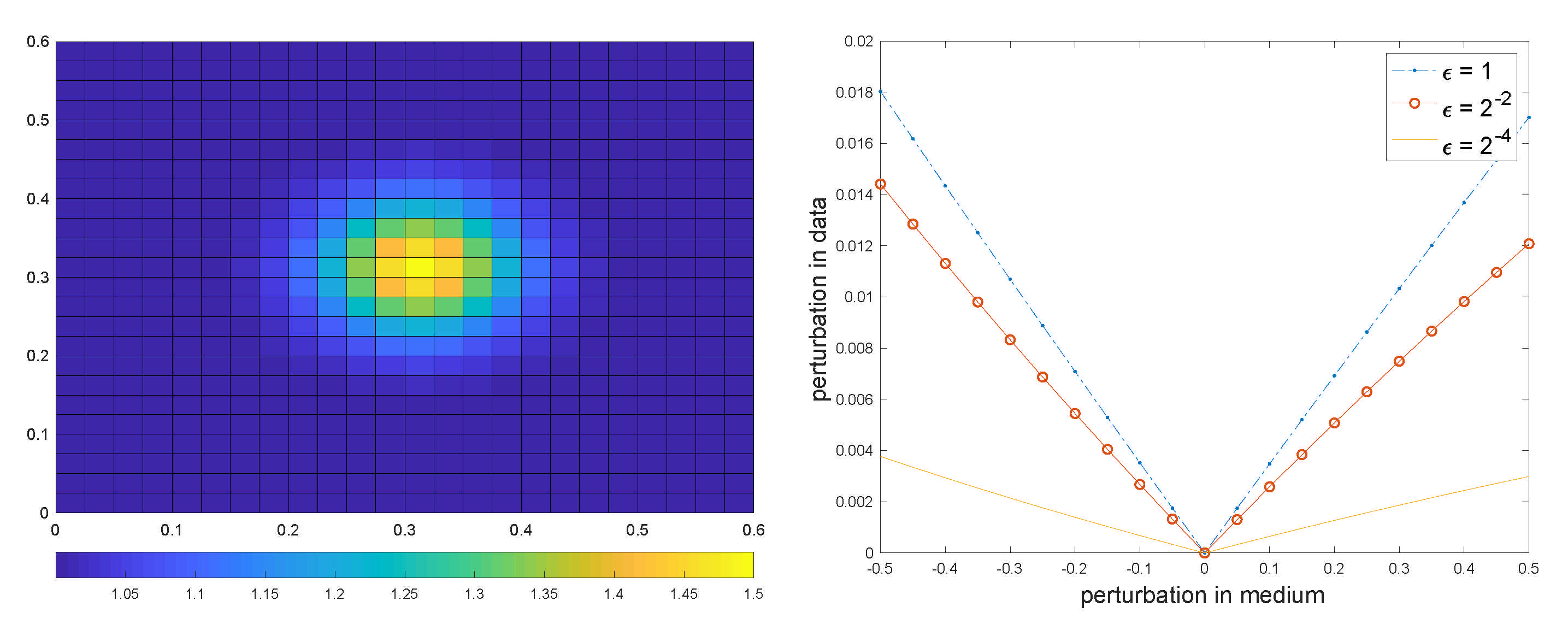
In the first test, we assume ${\sigma }_s\left(x\right)$ has the form

$${\sigma }_s\left(x\right)=1+\sigma \mathcal{N}((0.3,0.3),\mathsf{\Sigma }),$$

(57)

where $\mathcal{N}(0,\mathsf{\Sigma })$ is a two-dimensional normal distribution with mean zero and a fixed covariance matrix $\mathsf{\Sigma }$. The parameter $\sigma$ is the parameter to be inferred. We assume the ground-truth $\sigma =0.5$, and the ground-truth medium is plotted on the left of Figure 1. The inverse problem aims at inferring this ground-truth from the prescribed data pairs. To illustrate the stability of the inverse problem, we show how, for different choices of $\sigma$ away from the truth, the measurements differ from the true measurements. More precisely, we denote

$$d_p\left(\sigma \right)={\left(\sum _{i,j}{|d_{i,j}\left(\sigma \right)-d_{i,j}^{\mathrm{true}}|}^2\right)}^{1/2}$$

(58)

as the perturbation in the measurement, where $d_{i,j}$ is the measurement with a fixed $\sigma$ for the i-th experiment and j-th measurement, and $d_{i,j}^{\mathrm{true}}$ is the measurement with true $\sigma =0.5$. In the right panel of Figure 1, we plot the difference in measurement data (58) versus the perturbation in $\sigma$ for three different $ϵ$. It is clear that with smaller $ϵ$, the difference in measurement becomes more indistinguishable, which means that a smaller perturbation in measurement can lead to larger deviation in reconstruction. This is in consistent with our theory on the stability deterioration with decreasing $ϵ$.

Figure 1. Test 1. (Left): ground truth (57) with $\sigma =0.5$. (Right): perturbation in measured data versus perturbation in $\sigma$.

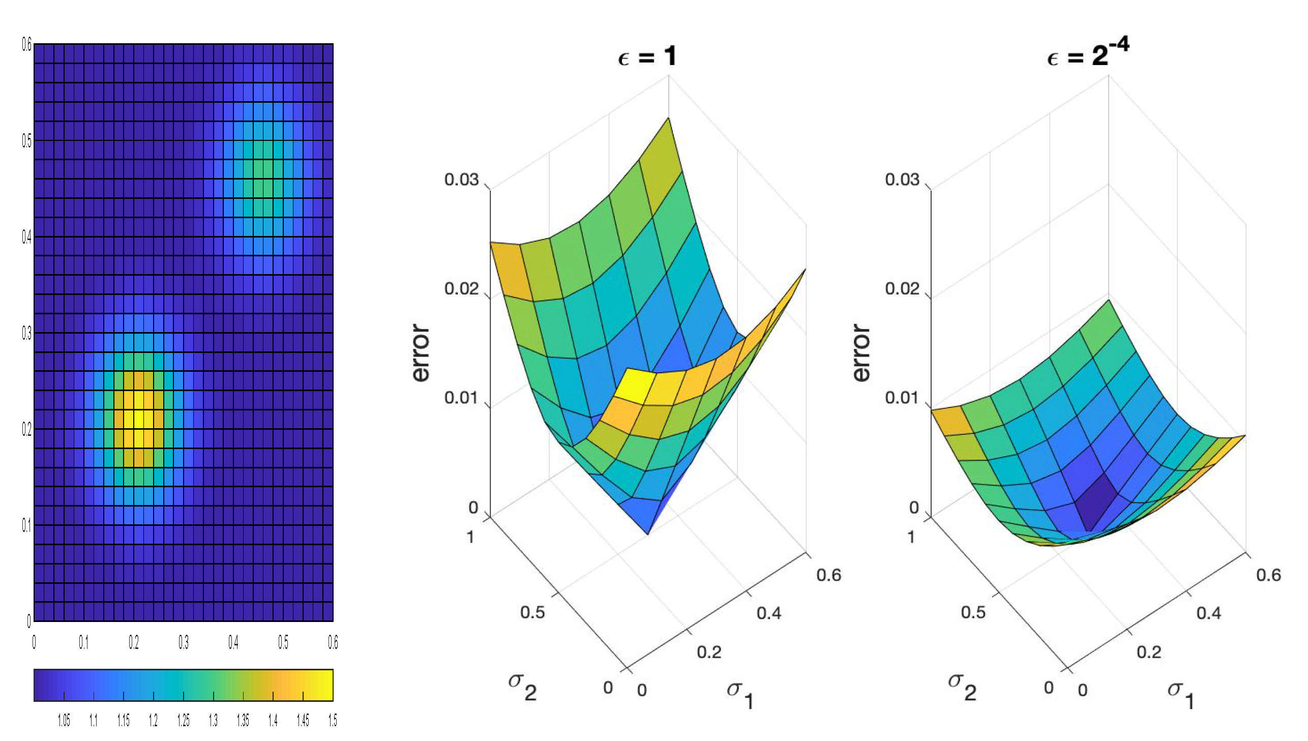
In the second test, we consider a different form of ${\sigma }_s\left(x\right)$:

$${\sigma }_s\left(x\right)=1+{\sigma }_1\mathcal{N}([0.2,0.2],\mathsf{\Sigma })+{\sigma }_2\mathcal{N}([0.45,0.45],\mathsf{\Sigma }).$$

(59)

Here, the to-be-reconstructed parameters are ${\sigma }_1$ and ${\sigma }_2$. We choose ${\sigma }_1=0.5$ and ${\sigma }_2=0.3$ to be the ground-truth and display the medium in Figure 2. Similar to the previous case, we plot the difference in measurement

$$d_p({\sigma }_1,{\sigma }_2)={\left(\sum _{i,j}{|d_{i,j}({\sigma }_1,{\sigma }_2)-d_{i,j}^{\mathrm{true}}|}^2\right)}^{1/2}$$

(60)

with respect to ${\sigma }_1\in (0,1)$ and ${\sigma }_2\in (0,0.6)$. It is again evident that for smaller $ϵ$, $d_p$ becomes flatter, leading to a deterioration in stability, as shown in Figure 2. In addition, we identify the data that are above $0.05\times {max}_{i,j}\left\{d_{i,j}\right\}$ in Figure 3. Here, the horizontal axis is the index for the experiment, and the vertical axis is the index for the receiver. It is seen that a larger $ϵ$ gives a sparse dataset, whereas small $ϵ$ gives a dense dataset, meaning that all receivers receive some information about the source. This indicates that the data are more spread out for smaller $ϵ$, which makes the inverse problem harder to solve.

Figure 2. Test 2: The panel on the left shows the ground-truth medium with ${\sigma }_1=0.5$ and ${\sigma }_2=0.3$ in (59). The two plots on the right show, for different $ϵ$, the perturbation in the measured data versus the perturbation in ${\sigma }_{1,2}$.

Figure 3. Test 2. Visualization of measured data whose intensity value is above $0.05\times {max}_{i,j}\left\{d_{i,j}\right\}$.

7. Conclusions

In this paper, we examine the stability deterioration for the multiscale inverse radiative transfer equation (RTE) in the Bayesian framework. Even though the instability on the continuous level was discussed in the literature [31] and the multiscale convergence was shown in [16,17,32], the instability representation in the Bayesian framework was open. The current paper constitutes the first result that fills the gap. The results presented suggest that one should not use Bayesian inference for conducting optical tomography when the photon energy is low. The numerical algorithm, without fine tuning, would carry very limited use in reconstructing the ground-truth media.