Analysis of Thermal Performances in a Ventilated Room Using LBM-MRT: Effect of a Porous Separation

Abstract

This article demonstrates the feasibility of porous separation on the performance of displacement ventilation in a rectangular enclosure. A jet of fresh air enters the cavity through an opening at the bottom of the left wall and exits through an opening at the top of the right wall. The porous separation is placed in the center of the cavity and its height varies between 0.2 and 0.8 with three values of thickness, 0.1, 0.2, and 0.3. The heat transfer rate was calculated for different intervals of Darcy (10⁻⁶ ≤ Da ≤ 10), Rayleigh (10 ≤ Ra ≤ 10⁶), and Reynolds (50 ≤ Re ≤ 500) numbers. The momentum and the energy equations were solved by the lattice Boltzmann method with multiple relaxation times (LB-MRT). Schemes D2Q9 and D2Q5 were chosen for the velocity and temperature fields, respectively. For porous separation, the generalized Darcy–Brinkman–Forchheimer model was adopted. It is represented by a term added in the standard LB equations. For the dynamic domain, numerical simulations revealed complex flow structures depending on all control parameters. The results showed that the thermal field, mainly in the second compartment, is very dependent on the size and permeability of the porous separation. However, they have no influence on the transfer rate.

1. Introduction

Heat transfer in enclosures has been of great interest to researchers due to the many applications arising from such geometries. Among the numerous works and papers published in the field of thermal flow in closed cavities, we cite the work of de Vahl Davies [1]. The latter considered as the reference work concerning heat transfer in a closed enclosure. The author considered a driving thermal gradient on the vertical walls, while the horizontal walls were considered adiabatic. The results have been validated several times and are considered as a benchmark for the case of closed cavities. Thereafter, Oztop [2] numerically analyzed the convective heat transfer in a porous rectangular enclosure inclined by a variable angle α. One of the side walls is kept at a constant temperature and another one is partially cooled, while the other walls are adiabatic. After solving by the finite volume method, he found that the tilt angle and the aspect ratio dominate the heat transfer evolution. In the same year, Sathiyamoorthy et al. [3] analyzed the natural convection in closed cavity using the finite volume method. The bottom wall is uniformly heated, but the vertical walls are linearly heated while the top wall is adiabatic. The results were presented for a Rayleigh number (10³ < Ra < 10⁵) and a Prandtl number (0.7 ≤ Pr ≤ 10). Varol et al. [4] studied the steady convection in a rectangular enclosure filled with a porous medium. The temperature profile in the base wall varies according to sinusoidal function, while the other walls are isolated. The problem was solved using a finite volume method, and the controls parameters are: Rayleigh number (10 ≤ Ra ≤ 1000), aspect ratio (0.25 ≤ AR ≤ 1.0), and amplitude of the temperature (0.25 ≤ λ ≤ 1.0). As the main result, they found that the increase in amplitude λ causes the increase in convective heat transfer, whereas decreases with the diminution of the aspect ratio. Ameziani et al. [5] added the effect of a moving wall on the thermal exchange by considering the cooperating and opposing forces of natural and forced convection. The authors found that a heat transfer minimum designated by the Nusselt number is observed for a specific pair of (Ra-Re). Huelsz and Rechtman [6] treated the heat transfer by the natural convection of air in a tilted, differentially heated square cavity. The simulation was carried out by the lattice Boltzmann method for a laminar regime with variation in the inclination angle and the Rayleigh number. The results show that for a given value of the Rayleigh number, a hysteresis is observed, whatever the value of the tilt angle.

In the case of ventilated cavities, the number of studies is rather abundant; in the last few years, we can cite the work of Omri and Nasrallah [7] on the transient mixed convection in the laminar regime. The cavity is cooled by a fresh fluid at a temperature lower than the initial temperature of the cavity. The governing equation was solved with a finite volume method. The dynamic and thermal fields are numerically resolute for a wide range of Re and Ri, and for different fluid inlet–outlet positions. In configuration (A), the results show that a single vortex turning in a clockwise direction is generated when Re increases with Ri < 1, or with an increase in Ri at moderate values of Re. However, the flow becomes multi-cellular when inertial and buoyancy effects are significant. In configuration B, increasing Ri reverses the fluid clockwise, but increasing Re reverses the fluid counterclockwise, and the dynamic field has several structures, depending on the values of the control parameters. Najam et al. [8] numerically studied the mixed convection in a T-shaped cavity heated with a constant heat flow and cooled with an air jet from the bottom. The heater blocks are identical, and the system is symmetrical about a vertical axis through the centers of the openings. A finite difference method was used to solve the governing equations. The results obtained for H/L = 1 indicate the existence of multiple solutions, and the heat transfer depends substantially on the control parameter values. Later, Gan [9] used CFD for the simulation of buoyancy-driven natural ventilation in a vertical enclosure for different heat flow intensities and wall thermal distributions using two computational domains. The simulation results show that the ventilation rate and the heat transfer coefficient depend on the inlet position as well as on the cavity size. For the case of ventilated cavities with porous media, studies are rather rare; we quote the work of Tong and Subramaniant [10], who studied natural considered convection in two rectangular cavities filled with porous media, with the goal to establish the heat transfer characteristics. The flow in the porous region was modelled by a modified revised Darcy’s law with the no-slip condition. Through the finite element solution, the authors concluded that there are regions wherein the heat transfer can be reduced by partially filling the cavity with the porous medium. A few years later, Moraga et al. [11] used the finite volume method (MVF) to study mixed convection in a ventilated rectangular cavity, vertically divided into two different porous media; they studied the effect of several control parameters such as the Darcy number, Reynolds number, Richardson number, aspect ratio, and flow direction. They found that the friction coefficient of the walls is larger when Re = 500 and Ri = 10 in both flow directions. Additionally, when the Darcy number increases, the velocity gradients increase near the walls, resulting in an increase in the friction coefficient (0 < Cf Re < 47). Thereafter, Mehrizi et al. [12] carried out a numerical analysis of heat transfer by forced convection in a ventilated cavity with an obstacle heated at a constant temperature. The walls of this cavity and the inlets/outlets are adiabatic. They used LBM for incompressible flow in a porous medium and the Darcy–Brinkman–Forchheimer model to consider the effect of the Reynolds number and Prandtl on the heat flow and temperature distribution. They found that increasing the Reynolds and Prandtl numbers enhanced the heat transfer characterized by the average Nusselt number. Oztop et al. [13] considered the natural convection heat transfer in a partially open cavity filled with porous media. They used the Darcy–Brinkman–Forcheimer model in the case where the left vertical wall had a constant temperature. They examined the different control parameters (porosity, Darcy number, Grashof number, and length of the heated wall). The authors found that the Nusselt number increases when the Grashof number increases, due to strengthening buoyancy-driven flows. In partially porous cavities also, Liu and He [14] are interested LBM-MRT modelling of incompressible flow. Porous medium is modeled by the Brinkman and Forchheimer models as extensions of the Darcy model. Additionally, through the Chapman–Enskog analysis, they were able to establish the generalized Navier–Stokes equations and found that their numerical results agreed with those findings with the analytical method. Shuja et al. [15] numerically studied heat transfer in a ventilated cavity with two porous blocks. The authors considered a moderate Reynolds number (Re = 100) over a large porosity range for two aspect ratios. The obtained results showed that the aspect ratio has little influence on the transfers which are directly dependent on the porosity. In second numerical research with the same configuration, the same authors [16] studied the flow field and heat transfer (Nusselt number). They showed that, for the first block (inlet fresh air side), the increase in Gr enhances the heat transfer and favors the natural convection phenomenon. Hireche et al. [17] performed a numerical analysis to determine the thermal convection characteristics in a ventilated rectangular cavity with an aspect ratio of (A = 2) and a porous partition in the middle. They concluded that heat transfer increases with an increase in Re and Ra values. Additionally, they concluded that the effect of the Darcy number is very significant for small permeability, while the effect of the porous layer height is hardly significant with a maximum deviation of less than 7%. Recently, several papers have been published on ventilated cavities, with different geometries and opening positions, even changing the physical properties of fluid [18,19,20,21,22,23,24,25,26].

From this synthesis, it can be seen that much of the numerical work has been carried out on ventilated cavities. For the case of displacement ventilation, few works have treated heat transfer in a rectangular room with a porous separation. However, most of the previous studies do not take into account the type of separation (solid or porous) and its dimensions (thickness and height), parameters on which this work is based—in particular, the separation thickness. In this paper, we explore the possibility of modeling the heat removal process by displacement ventilation in professional premises, large rooms, open plan offices, or general hospital divisions, providing air exchange and being among the most efficient systems. It presents an interesting solution for enhancing air quality, energy saving, and thermal comfort in buildings.

2. Mathematical Formulation

The present study focuses on convection in a rectangular open cavity of height H and length L = 2H, as shown in Figure 1, partitioned by a vertical porous wall of thickness “e” varying between H/10 and 3H/10 as well as a height that varies between H/5 and 4H/5. The porous wall is saturated by a single fluid. The air in the cavity is renewed through two diametrically opposed openings located at the lower and upper corners of the left and right walls, respectively. The walls of the cavity are impermeable, so the left wall is heated at a constant temperature and the other walls are adiabatic.

Some assumptions have been considered to simplify the mathematical formulation of our model. The fluid is Newtonian and incompressible. The fluid flow into the cavity is laminar and two-dimensional, while the Boussinesq approximation has been applied to model the density variations. The porous bloc is assumed to be homogeneous, isotropic, and in thermodynamic equilibrium with the fluid. The thermo-physical properties of fluid are considered constant over the temperature scale. It is also assumed that radiative transfer is neglected.

2.1. Governing Equations

2.1.1. Fluid Zone

The equation of continuity expresses the theory of mass conservation of a moving fluid. In an elementary volume, the mass of the fluid removed or injected is equal to the sum of the variation fluid density in an elementary time interval, and the mass flows through the surface of this volume. The transport equations express the theory of momentum and energy conservation. They are defined as:

• Continuity equation:

$$\nabla \cdot u=0$$

(1)

• Equation of momentum conservation:

  $${\rho }_f\underset{1}{\underbrace{\left[\frac{\partial u}{\partial t}+u\nabla \left(u\right)\right]}}=\underset{2}{\underbrace{-\nabla P}}+\underset{3}{\underbrace{\mu {\nabla }^{2}u}}+\underset{4}{\underbrace{{\rho }_{f}G}},$$

  (2)

  where:

  (1)

  Macroscopic inertial forces;

  (2)

  Pressure gradient;

  (3)

  Diffusion term;

  (4)

  Volume force, where the density is expressed according to the Boussinesq approximation.

• Equation of energy conservation:

$${\rho }_f{c}_p\left[\frac{\partial T}{\partial t}+u\nabla \left(T\right)\right]=\nabla \left(k_f\nabla T\right)$$

(3)

where:

c_p: Specific heat.

k_f: Fluid conductivity.

2.1.2. Porous Zone

Based on the generalized Darcy–Brinkman–Forchheimer model, the dimensional governing equations for convection heat transfer in a homogeneous, isotropic, and fluid-saturated porous medium can be written as [27,28,29]:

• Continuity equation:

$$\epsilon \frac{\partial {\rho }_f}{\partial t}+\nabla \left({\rho }_f\hspace{0.17em}u\right)=0$$

(4)

• Equation of momentum conservation:

  $${\rho }_f\underset{1}{\underbrace{\left[\frac{\partial u}{\partial t}+u\nabla \left(u\right)\right]}}=\underset{2}{\underbrace{-\nabla P}}+\underset{3}{\underbrace{{\mu }_{eff}{\nabla }^{2}u}}-\underset{4}{\underbrace{\frac{\upsilon }{K}u}}-\underset{5}{\underbrace{\frac{1.75}{\epsilon \sqrt{150\epsilon K}}\left|u\right|u}}+\underset{6}{\underbrace{{\rho }_{f}G}}$$

  (5)

  (1)

  Macroscopic inertial forces;

  (2)

  Pressure gradient;

  (3)

  Brinkman’s viscous term;

  (4)

  Darcy term;

  (5)

  Forchheimer term (microscopic inertial forces [30]);

  (6)

  Volume forces.

• Equation of energy conservation:

$${\left({\rho }_0{c}_p\right)}_m\frac{\partial T}{\partial t}+{\left({\rho }_0{c}_p\right)}_f\nabla \left(Tu\right)=\nabla \left(k_{eff}\nabla T\right)$$

(6)

where ${\left({\rho }_0{c}_p\right)}_m$ and ${\left({\rho }_0{c}_p\right)}_f$ are, respectively, the thermal heat capacity of the porous medium and the fluid, respectively, and k_eff is the effective thermal conductivity.

2.2. Dimensionless Equations

Governing equations are written in dimensionless form using the reduced variables:

$$X=\frac{x}{H}\hspace{0.17em},\hspace{0.17em}\hspace{0.17em}Y=\frac{y}{H}\hspace{0.17em},\hspace{0.17em}\hspace{0.17em}U=\frac{u}{U_0}\hspace{0.17em},\hspace{0.17em}\hspace{0.17em}V=\frac{v}{U_0}\hspace{0.17em},\hspace{0.17em}\hspace{0.17em}P=\frac{p}{\rho U_0^2}\hspace{0.17em},\hspace{0.17em}\hspace{0.17em}\theta =\frac{T-T_c}{∆T},\hspace{0.17em}\hspace{0.17em}∆T=T_h-T_c,\hspace{0.17em}\hspace{0.17em}\mathrm{t}=\frac{t}{H/U_0}$$

(7)

The governing equations system is given in dimensionless form in the next section.

2.2.1. Fluid Zone

• Continuity equation:

$$\frac{\partial U}{\partial X}+\frac{\partial V}{\partial Y}=0$$

(8)

• Equation of momentum conservation following $X$

$$\frac{\partial U}{\partial t}+\left[U\frac{\partial U}{\partial X}+V\frac{\partial U}{\partial Y}\right]=-\frac{\partial P}{\partial X}+\frac{1}{\mathrm{Re}}\left(\frac{{\partial }^{2}U}{\partial X^2}+\frac{{\partial }^{2}U}{\partial Y^2}\right)$$

(9)

• Equation of momentum conservation following $Y$:

$$\frac{\partial V}{\partial t}+\left[U\frac{\partial V}{\partial X}+V\frac{\partial V}{\partial Y}\right]=-\frac{\partial P}{\partial Y}+\frac{1}{\mathrm{Re}}\left(\frac{{\partial }^{2}V}{\partial X^2}+\frac{{\partial }^{2}V}{\partial Y^2}\right)+\frac{Ra}{\mathrm{Pr}\cdot \mathrm{Re}}\theta$$

(10)

• Equation of energy conservation:

$$\frac{\partial \theta }{\partial t}+\frac{\partial \left(U\theta \right)}{\partial X}+\frac{\partial \left(V\theta \right)}{\partial Y}=\frac{1}{\mathrm{Re}\mathrm{Pr}}\left(\frac{{\partial }^2\theta }{\partial X^2}+\frac{{\partial }^2\theta }{\partial Y^2}\right)$$

(11)

2.2.2. Porous Zone

• Continuity equation:

$$\frac{\partial U}{\partial X}+\frac{\partial V}{\partial Y}=0$$

(12)

• Equation of momentum conservation following $X$ [30]:

$$\frac{\partial U}{\partial t}+\left[\frac{U}{\epsilon }\frac{\partial U}{\partial X}+\frac{V}{\epsilon }\frac{\partial U}{\partial Y}\right]=-\frac{\partial \epsilon P}{\partial X}-\frac{1}{Da\mathrm{Re}}U-\frac{1.75}{\sqrt{150}}\frac{{\left(U^2+V^2\right)}^{1/2}}{\sqrt{Da}}V+\frac{1}{\mathrm{Re}}\left(\frac{{\partial }^{2}U}{\partial X^2}+\frac{{\partial }^{2}U}{\partial Y^2}\right)$$

(13)

• Equation of momentum conservation following $Y$ [30]:

$$\frac{\partial V}{\partial t}+\left[\frac{U}{\epsilon }\frac{\partial V}{\partial X}+\frac{V}{\epsilon }\frac{\partial V}{\partial Y}\right]=-\frac{\partial \epsilon P}{\partial Y}-\frac{1}{Da\mathrm{Re}}V-\frac{1.75}{\sqrt{150}}\frac{{\left(U^2+V^2\right)}^{1/2}}{\sqrt{Da}}V+\frac{1}{\mathrm{Re}}\left(\frac{{\partial }^{2}V}{\partial X^2}+\frac{{\partial }^{2}V}{\partial Y^2}\right)+\frac{Ra}{\mathrm{Pr}\cdot \mathrm{Re}}{\theta }_{ }$$

(14)

• Equation of energy conservation:

$$\gamma \frac{\partial \theta }{\partial t}+\frac{\partial \left(U\theta \right)}{\partial X}+\frac{\partial \left(V\theta \right)}{\partial Y}=\frac{R_k}{\mathrm{Re}\mathrm{Pr}}\left(\frac{{\partial }^2\theta }{\partial X^2}+\frac{{\partial }^2\theta }{\partial Y^2}\right)$$

(15)

where γ and R_k are, respectively, the heat capacity ratio and the thermal conductivity ratio. In our work, they have been assumed unit values.

The non-dimensional form of the latter equations gives the appearance of the following non-dimensional parameters mentioned in

Table 1. Dimensionless number expressions.

Types	Expression
Prandtl number	$\mathrm{Pr}=\upsilon /\alpha$
Reynolds number	$\mathrm{Pr}=U_{0}H/\upsilon$
Rayleigh number	$\mathrm{Ra}=(g\beta ∆T_{ref}{H}^3)/\upsilon \alpha$
Darcy number	$Da=K/H^2$

.

The hydrodynamic boundary conditions, characterized by the non-slip condition of the fluid particles on the solid walls and their impermeability, are given:

$$\mathrm{Left} \mathrm{vertical} \mathrm{wall}: U\left(0,Y\right)=V\left(0,Y\right)=0\hspace{0.17em};\hspace{1em}0.1\le Y\le 1$$

(16)

$$\mathrm{Right} \mathrm{vertical} \mathrm{wall}: U\left(2,Y\right)=V\left(2,Y\right)=0\hspace{0.17em};\hspace{1em}0\le Y\le 0.9$$

(17)

$$\mathrm{Horizontal} \mathrm{surfaces}: U\left(X,0\right)=V\left(X,0\right)=U\left(X,1\right)=V\left(X,1\right)=0\hspace{0.17em};\hspace{1em}0\le X\le 2$$

(18)

$$\mathrm{The} \mathrm{inlet}: \{\begin{array}{l}X=0\\ 0\le Y\le 0.1\end{array}\hspace{0.17em}\hspace{1em}U=1\hspace{0.17em},\hspace{1em}V=0\hspace{0.17em}.$$

(19)

$$\mathrm{The} \mathrm{outlet}: \{\begin{array}{l}X=2\\ 0.9\le Y\le 1\end{array}\hspace{0.17em}\hspace{1em}\frac{\partial U}{\partial X}=0\hspace{0.17em},\hspace{1em}V=0\hspace{0.17em}.$$

(20)

Thermal boundary conditions:

$$\mathrm{Left} \mathrm{vertical} \mathrm{wall}: \hspace{0.17em}X=0;\hspace{0.17em}\hspace{0.17em}\hspace{0.17em}\hspace{0.17em}0.1\le Y\le 1,\hspace{1em}\theta =1$$

(21)

$$\mathrm{The} \mathrm{inlet}: \hspace{0.17em}\hspace{0.17em}\hspace{0.17em}\theta =0,\hspace{0.17em}\hspace{0.17em}\hspace{0.17em}\hspace{0.17em}0\le Y\le 0.1$$

(22)

$$\mathrm{Right} \mathrm{vertical} \mathrm{wall}: X=2,\hspace{1em}0\le Y\le 0.9,{\hspace{1em}\frac{\partial \theta }{\partial X}|}_{X=2}=0$$

(23)

$$\mathrm{The} \mathrm{outlet}: \hspace{1em}\frac{\partial \theta }{\partial X}=0,\hspace{0.17em}\hspace{0.17em}\hspace{0.17em}0.9\le Y\le 1$$

(24)

$$\mathrm{Horizontal} \mathrm{surfaces}: {\frac{\partial \theta }{\partial Y}|}_{Y=0}=0\hspace{0.17em},{\hspace{0.17em}\frac{\partial \theta }{\partial Y}|}_{Y=1}=0\hspace{0.17em};\hspace{1em}0\le X\le 2$$

(25)

Finally, we express the heat transfer rate on the active surface by the averaged and local Nusselt numbers, defined, respectively, as:

$$Nu={{\displaystyle {\int }_{\frac{a}{H}}^{\hspace{0.17em}1}N{u}_X\partial Y}}_{ }$$

(26)

with:

$$N{u}_X={\frac{\partial \theta }{\partial X}|}_{X=0}$$

(27)

3. Lattice Boltzmann Method

The Boltzmann method on lattice, commonly called the LBM (lattice Boltzmann method), is another approach for numerical simulation of physical phenomena. It is a relatively new method that differs from traditional methods. The construction of the Boltzmann method on a lattice is represented by two independent steps: the development of statistical physics and the appearance of cellular automata [31,32]. In 1872, Boltzmann proposed his famous equation describing the spatio-temporal evolution of a function f representing the distribution of particles with a given velocity at a given place and time. This function is often named the distribution function and thus depends on time, space, and velocity:

$$\frac{\partial f}{\partial t}+c_i\frac{\partial f}{\partial x_i}+\frac{F_i}{m}\frac{\partial f}{\partial c_i}={\left(\frac{\partial f}{\partial t}\right)}_{coll}$$

(28)

The right side of the Boltzmann equation, called the collision operator, represents the influence of collisions between particles. If this term is equal to zero, the particles are simply affected and subjected to the action of the force F present on the left-hand side. If the particles collide, the evolution of the system depends on the form of the collision operator.

The work of Chapman [33] and Enskog [34], validated experimentally by the chemist FW Dootson, led to direct relations between the Boltzmann equation and those of Navier–Stokes (1823), thus extending the work of Boltzmann. However, the collision operator chosen by Chapman and Enskog remained very complex and typic. It was then necessary to wait many decades until the development of a simple collision model; it was the mathematicians Bhatnagar, Gross, and Krook who gave birth to it in 1954 [35]. This model, established from complex theoretical developments, is based on the idea that a particle collision can be described as the relaxation in a given time of the particles, towards a given equilibrium state. This fundamental idea makes it possible to write the collision operator in a very simple form that is named the BGK operator, from the name of its creators. Statistical physics showed, as early as 1954, that the Boltzmann equation provided with the BGK operator could be used to describe fluid mechanics flows governed by the Navier–Stokes equations. The Boltzmann method on lattices could have been born at that time, but the notion of discretization and networking, specific to computer use, only emerged much later with the intensive development of numerical simulation.

In what follows, we will not consider any external force (Fi), and the effects of gravity will be neglected. We notice that the density, momentum, and kinetic energy of the fluid are found by considering all possible speeds:

$$\rho ={\displaystyle \int ƒ}dc$$

(29)

$$\rho u={\displaystyle \int cƒ}dc$$

(30)

$$\rho e=\frac{1}{2}{\displaystyle \int {\left|c-u\right|}^{2}mƒdc}$$

(31)

Considering only binary collisions transforms the velocities [c₁; c₂] (pre-collision) into [c₁′; c₂′] (post-collision). In the absence of a collision, the particles are in thermodynamic equilibrium. Such a state is described by an equilibrium distribution function f^eq, a solution to the equation:

$${\left(\frac{\partial f}{\partial t}\right)}_{coll}=\Omega$$

(32)

Such a function therefore verifies:

$${ƒ}_i^{eq}=w_i\rho {\left[1+3\left(c_i\cdot u\right)+\frac{9}{2}{\left(c_i\cdot u\right)}^2-\frac{3}{2}{u}^2\right]}_{ }$$

(33)

where:

w_i: network constants;

C: speed of sound.

3.1. Discretization of the Lattice Boltzmann Equation

The lattice Boltzmann method can be applied for the simulation of fluid flow, heat, and mass transfer. The fluid is considered as a set of particles, moving at a discrete velocity in specified directions, according to the lattice structure, and colliding (interact) with each other at the nodes of the lattice. The distribution function is the probability of the presence of a particle at a certain node with a certain velocity. The collision and propagation of particles is governed by the Boltzmann equation of the lattice, which reflects the evolution of these functions. The external force implemented by a source term:

$$f_i(x+e_i{\delta }_t,t+{\delta }_t)-f_i(x,t)=\Omega \hspace{0.17em}\left(f_i\right)+{\delta }_t{F}_i$$

(34)

where $f_i$ is the distribution function with the velocity $e_i$ at the lattice node x at time t,${\delta }_t$ is the discrete time step, $\Omega \hspace{0.17em}\left(f_i\right)$ is the discrete collision operator, and $F_i$ is the external forces term.

Collision Operator

There are several approaches to calculating the collision operator, such as:

(a)

The BGK approximation:

Bhatnagar, Gross, and Krook (BGK) developed a simplified model of the collision operator in 1954 [35]. The collision operator can be written as follows:

$$\Omega =\omega \left({ƒ}_{}^{eq}-ƒ\right)=\frac{1}{\tau }\left({ƒ}_{}^{eq}-ƒ\right)$$

(35)

$$\omega =\frac{1}{\tau }$$

(36)

τ: relaxation factor;

ω: collision frequency.

The local distribution function is denoted by f^eq, which is the Maxwell–Boltzmann distribution function.

The Boltzmann equation (without external forces) can be written after the application of the BGK approximation, as follows:

$$\frac{\partial f}{\partial t}+c\cdot \nabla f=\frac{1}{\tau }\left({ƒ}_{}^{eq}-ƒ\right)$$

(37)

The discrete velocity of Boltzmann equation can be written as follows:

$$\frac{\partial f_i}{\partial t}+c_i\cdot \nabla f_i=\frac{1}{\tau }\left({ƒ}_i^{eq}-{ƒ}_i\right)$$

(38)

The discretization of the previous equation gives us:

$$f_i\left(x+c_i\Delta t,t+\Delta t\right)=f_i\left(x,t\right)+\frac{\Delta t}{\tau }\left[f_i^{eq}\left(x,t\right)-f_i^{}\left(x,t\right)\right]$$

(39)

(b)

Multiple Relaxation time MRT:

In order to overcome these deficiencies of the LBGK model (numerical instability, applicable only for Pr = 1), d’Humières [36] proposes the approach of moment, known as the multiple relaxation time model. To simulate the evolution of macroscopic quantities, different relaxation times are used. By running the collision in an orthogonal space–time, an efficient and flexible scheme is obtained. This model has optimal stability compared to the BGK model. In the MRT scheme, the collision term is written as [37]:

$${\Omega }_i=-M^{-1}{S}_i\left[m_i(x,t)-m_i{}^{eq}(x,t)\right]$$

(40)

Therefore, the Boltzmann equation is written as:

$$f_i\left(x+c_i\Delta t,t+\Delta t\right)-f_i\left(x,t\right)=-M^{-1}{S}_i\left[m_i\left(x,t\right)-m_i^{eq}\left(x,t\right)\right]$$

(41)

The velocity is equal to the ratio between displacement dx and the unit time dt. $m(x,t)=et m_i^{eq}(x,t)$ are moment vectors; $m={(m_0,m_1,m_2, \dots ,m_n)}^T$. The relaxation matrix is a diagonal matrix, and the linkage between velocities and moment spaces is given from linear transformation as follows:

$$m=M\cdot f$$

(42)

$$f=M^{-1}m$$

(43)

3.2. Dynamic Lattice Boltzmann Model

The terminology used in the LBM method to describe the dimension and number of model directions is as follows: DnQm, where: n and m designate the problem dimension (1D, 2D, and 3D) and the number of the function directions (discrete velocities).

3.2.1. The Two-Dimensional Nine-Speed Model (D2Q9)

This is the most widely used model, especially for the study of flow problems. The D2Q9 model is based on a square lattice of step $\delta x=\delta y=1$, and each lattice pattern is characterized by nine discrete velocities c_i(i = 0, …, 8) [38].

For the hydrodynamic field, the two-dimensional nine-velocity D2Q9 model is used in this work as well as the Boltzmann equation of the multi-relaxation time lattice (MRT-LBM) [39,40]:

$$f_i\left(x+e_i\delta t,t+\delta t\right)-f_i\left(x,t\right)=-M^{-1}{S}_i{\left[m_i\left(x,t\right)-m_i^{eq}\left(x,t\right)\right]}_{ }$$

(44)

The nine discrete velocities are given by:

$$e_i=\{\begin{array}{l}\left(0,0\right)\hspace{1em}\hspace{1em}\hspace{1em}\hspace{1em}\hspace{1em}\hspace{1em}\hspace{1em}\hspace{1em}\hspace{1em}\hspace{1em}\hspace{1em}\hspace{1em}\hspace{1em}i=0\\ \left[\cos \varphi ,\sin \varphi \right]c\hspace{1em}\hspace{1em}\hspace{1em}\varphi =\left(i-1\right)\frac{\pi }{2}\hspace{1em}\hspace{1em}i=1,2,3,4\\ \left[\cos \varphi ,\sin \varphi \right]\sqrt{2}c\hspace{1em}\hspace{1em}\varphi =\left(2i-9\right)\frac{\pi }{4} \hspace{1em}i=5,6,7,8\end{array}$$

(45)

where $c=\delta x/\delta t=\delta y/\delta t$ is the lattice velocity, in which $\delta x/\delta t$ and $\delta y/\delta t$ are the lattice cell widths; these quantities are chosen equal to the unit $\delta x=\delta y=\delta t=1$.

The distribution function of local equilibrium $f_i^{eq}$ for the hydrodynamic field in porous media is calculated by equation:

$$f_i^{eq}=w_i\rho {\left(1+3e_{i}v+\frac{9{\left(e_{i}v\right)}^2}{2\epsilon }+\frac{3v^2}{2\epsilon }\right)}_{ }$$

(46)

where the weighting factors w_i are given in the literature as follows: $w_0=\frac{4}{9};w_{1-4}=\frac{1}{9};w_{5-8}=\frac{1}{36}$.

M as the transformation matrix, which projects f_i and f_i^eq into space–time with m = MF and m^eq = MF^eq, where m and m^eq are vectors of macroscopic and macroscopic equilibrium variables, respectively. The distribution functions in space–time are given by:

$$m=\left(\begin{array}{c}\rho \\ e\\ \phi \\ j_x-\frac{{\delta }_t}{2}\rho F_x\\ q_x\\ j_y-\frac{{\delta }_t}{2}\rho F_y\\ q_y\\ p_{xx}\\ p_{xy}\end{array}\right)=\left[\begin{array}{ccccccccc}1& 1& 1& 1& 1& 1& 1& 1& 1\\ -4& -1& -1& -1& -1& 2& 2& 2& 2\\ 4& -2& -2& -2& -2& 1& 1& 1& 1\\ 0& 1& 0& -1& 0& 1& -1& -1& 1\\ 0& -2& 0& 2& 0& 1& -1& -1& 1\\ 0& 0& 1& 0& -1& 1& 1& -1& -1\\ 0& 0& -2& 0& 2& 1& 1& -1& -1\\ 0& 1& -1& 1& -1& 0& 0& 0& 0\\ 0& 0& 0& 0& 0& 1& -1& 1& -1\end{array}\right]\hspace{0.17em}\hspace{0.17em}\left(\begin{array}{c}{f}_0\\ f_1\\ f_2\\ f_3\\ f_4\\ f_5\\ f_6\\ f_7\\ f_8\end{array}\right)=Mf$$

(47)

where ρ is the fluid density, e is related to the energy, φ is related to the square of the energy, j_x,y are the kinetic momentum components j = (j_x,j_y) = (ρv_x,ρv_y), q_x,y correspond to the energy flow in two directions, and p_xx,xy correspond to the diagonal and off-diagonal components of the stress rate tensor.

The density ρ and the momentum j_x,y are conserved quantities, while the other six velocity moments are not conserved. The equilibrium moments for the non-conserved moments m^eq can be defined as [41]:

$$e^{eq}=-2\rho +\frac{3{\rho }_0{\left|v\right|}^2}{\epsilon }\hspace{0.17em}\hspace{0.17em};\hspace{0.17em}\hspace{0.17em}{\varphi }^{eq}=\rho -\frac{3{\rho }_0{\left|v\right|}^2}{\epsilon }\hspace{0.17em}\hspace{0.17em};\hspace{0.17em}\hspace{0.17em}{q}_x^{eq}=-{\rho }_0{v}_x\hspace{0.17em}\hspace{0.17em};q_y^{eq}=-{\rho }_0{v}_y\hspace{0.17em}\hspace{0.17em};\hspace{0.17em}\hspace{0.17em}{p}_{xx}^{eq}=\frac{{\rho }_0\left(v_x^2-v_y^2\right)}{\epsilon }\hspace{0.17em}\hspace{0.17em};\hspace{0.17em}\hspace{0.17em}{p}_{xy}^{eq}=\frac{{\rho }_0{v}_x{v}_y}{\epsilon }$$

(48)

In the above equilibrium moments, the incompressibility approximation has been used, the fluid density is written as ρ = ρ₀ + δρ ≈ δ₀ (δρ is the density fluctuation), and (j_x,j_y ≈ ρ₀v). The average density of the fluid ρ₀ is taken to be 1 to simplify the model. I is the identity matrix and S is a diagonal relaxation matrix given by:

$$S=diag\left(s_0,\hspace{0.17em}{s}_1,\hspace{0.17em}{s}_2,\hspace{0.17em}{s}_3,\hspace{0.17em}{s}_4,\hspace{0.17em}{s}_5,\hspace{0.17em}{s}_6,\hspace{0.17em}{s}_7,\hspace{0.17em}{s}_8\right)$$

(49)

S_i are the relaxation rates. These values must be between 0 and 2 to keep the model stable. In our simulations, they are considered as follows:

$$S=diag{\left(1,\hspace{0.17em}1.2,\hspace{0.17em}1.4,\hspace{0.17em}1,\hspace{0.17em}1.2,\hspace{0.17em}1,\hspace{0.17em}1.2,\hspace{0.17em}\frac{1}{\tau },\hspace{0.17em}\frac{1}{\tau }\right)}_{ }$$

(50)

In the LBM-MRT method, the fluid kinematic viscosity is related to the relaxation parameter of the flow field by the following relation:

$$\upsilon =\frac{1}{3}\left(\tau -\frac{1}{2}\right)$$

(51)

The macroscopic fluid variables, density and velocity, are calculated as follows:

Mass conservation can be described as the summation of the distribution functions in each the lattice node, which represent the macroscopic density of the fluid [42]:

$$\rho ={\displaystyle \sum _{i=0}^8{f}_i}$$

(52)

The conservation of momentum can be described as the summation of the product of the microscopic lattice velocities by the distribution function:

$$\rho u={\displaystyle \sum _{i=0}^8{f}_i}{e}_i$$

(53)

Thus:

$$u=\frac{1}{\rho }{\displaystyle \sum _{i=0}^8{f}_i}{e}_i$$

(54)

3.2.2. D2Q5-MRT-LB Equation for the Thermal Field

For the temperature field, the two-dimensional model D2Q5 with five discrete velocities is used in our work.

The LBM-MRT equation can be written as follows:

$$g_i\left(x+e_i\delta t,t+\delta t\right)-g_i\left(x,t\right)=-N^{-1}{E}_i{\left[n_i\left(x,t\right)-n_i^{eq}\left(x,t\right)\right]}_{ }$$

(55)

where g_i(x,t) is the temperature distribution function. In the D2Q5 model, the five discrete speeds are given by the following relation:

$$e_i=\{\begin{array}{l}\left(0,0\right)\hspace{1em}\hspace{1em}\hspace{1em}\hspace{1em}\hspace{1em}\hspace{1em}\hspace{1em}\hspace{1em}\hspace{1em}\hspace{1em}\hspace{1em}\hspace{1em}i=0\\ \left[\cos \varphi ,\sin \varphi \right]c\hspace{1em}\hspace{1em}\varphi =\left(i-1\right)\frac{\pi }{2}\hspace{1em}\hspace{1em}i=1,2,3,4\end{array}$$

(56)

The equilibrium distribution function is given by:

$$g_i^{eq}=w_{i}T{\left[1+5e_{i}v\right]}_{ }$$

(57)

Here, the weighting factors w_i are given as follows; $w_0^{\prime }=3/5; w_{1-4}^{\prime }=1/10$.

N is an orthogonal transformation matrix 5 × 5, which projects g_i and g_i^eq into space–time with n = Ng and n^eq = Ng^eq, where n and n^eq are, respectively, the variables of macroscopic and macroscopic equilibrium temperature.

For temperature, the distribution functions in space–time are given by [43]:

$$n=\left(\begin{array}{c}{n}_0\\ n_1\\ n_2\\ \begin{array}{l}{n}_3\\ n_4\end{array}\end{array}\right)=\left|\begin{array}{ccccc}1& 1& 1& 1& 1\\ 0& 1& 0& -1& 0\\ 0& 0& 1& 0& -1\\ -4& 1& 1& 1& 1\\ 0& 1& -1& 1& -1\end{array}\right|\left(\begin{array}{c}{g}_0\\ g_1\\ g_2\\ \begin{array}{l}{g}_3\\ g_4\end{array}\end{array}\right)=N{g}_{ }$$

(58)

E is the diagonal relaxation matrix:

$$E=diag\left(r_0,r_1,r_2,r_3,r_4\right)$$

(59)

To ensure good stability of computation, the relaxation rates are chosen in our work as follows:

$$E=diag\left(1,\hspace{0.17em}1/{\tau }_T,\hspace{0.17em}1/{\tau }_T,\hspace{0.17em}1.25,\hspace{0.17em}1.25\right)$$

(60)

where ${\tau }_T$ M is the relaxation parameter of temperature field.

The collision process D2Q5 LBM-MRT proceeds as follows:

$$n_i^{*}(x,t)=n_i(x,t)-E\hspace{0.17em}\hspace{0.17em}\left[n_i(x,t)-n_i{}^{eq}(x,t)\right]$$

(61)

Between the five moments, only the temperature is kept:

$$n_0=T={{\displaystyle \sum _{i=0}^8{g}_i}}_{ }$$

(62)

In equilibrium, the non-conserved moments $n^{eq}=N{g}^{eq}$ are written as follows [44]:

$$n_1^{eq}=v_{x}T;\hspace{0.17em}{n}_2^{eq}=v_{y}T;\hspace{0.17em}{n}_3^{eq}=\varpi T;\hspace{0.17em}{n}_4^{eq}=0$$

(63)

3.3. Boundary Condition

The hydrodynamic boundary conditions that govern our problem are mainly the adherence of the fluid to all walls as well as a horizontal imposed inlet velocity and a velocity establishment on the outlet opening. For the thermal boundary conditions, we have an active left wall (hot temperature) with an insulation of all other walls. We also consider a fresh air source (cold temperature) at the inlet with a thermal establishment at the outlet. One of the most important parts of a Boltzmann lattice simulation is the establishment of boundary conditions. The establishment of boundary conditions for classical computational methods used in hydrodynamics (CFD) is carried out by obtaining the flow variables. This is not the case for the LBM method, where the distributions functions entered in the domain must be determined. Therefore, the appropriate equations for calculating of distribution functions at the domain boundary for each boundary condition.

In our work, we used the rebound boundary condition [45,46,47,48] to model the adhesion to all walls. We also used the boundary conditions for the imposed velocity type (Zu and He [42]) to model the imposed velocities and temperatures.

4. Validation of the Calculation Code

To validate our computational code, we compared our results with previous work (those of Rahman et al. [49]). The latter have studied mixed convection in a ventilated square cavity with a horizontal heat square block; the Richardson number for this study varies from 0.0 to 5.0, the Reynolds number has been fixed at Re = 100, and the fluid in the cavity is the air with Pr = 0.71. The comparison of results (Nusselt number at the hot wall) obtained from our computational code and those of the author considered was performed for the zero-dimensional limiting case of the obstacle, for different Richardson numbers (Figure 2). The confrontation shows a good agreement between our numerical simulations and those of the previous author.

5. Results and Interpretations

The required number of lattices is obtained through a grid sensitivity analysis to ensure accurate results. Due to the multiple parameters controlling the flow pattern, temperature field, and heat transfer, all calculations were performed by setting a constant Prandtl number (Pr = 0.71; the air) and a finite aspect ratio A = 2. The Reynolds number varies up to 500 and the Rayleigh number up to 10⁶. The ratio of conductivities and the ratio of viscosities between the fluid and porous media are equal to unity.

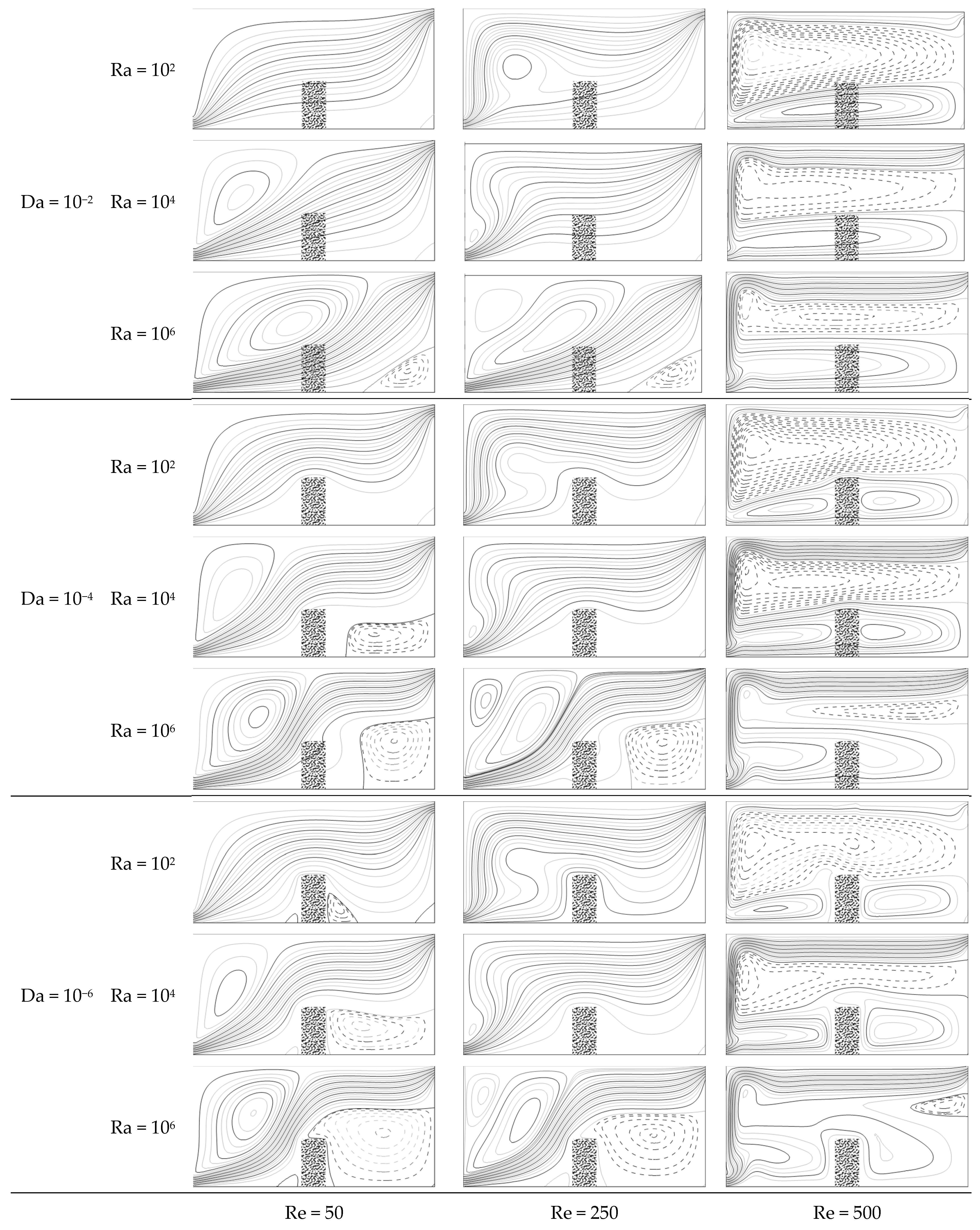
Figure 3 shows the stream functions (tangent to velocity vector) for different Darcy numbers, Rayleigh numbers, and for three Reynolds values. Note that the negative values of the stream functions are shown as dotted lines and that the porous medium thickness is taken to be constant at Ep = 0.2. In order to cover all the ranges considered, three values of Darcy are taken (10⁻²; fluid regime 10⁻⁴ low-permeability medium and Da = 10⁻⁶ for the Darcian regime). The Rayleigh number is assumed in the range of 10²–10⁶ in order to sweep from the diffusive to the convective regime. When Da = 10⁻² (fluid regime), the porous medium does not offer resistance to the fluid. As a result, the stream lines are continuous, and no distortion is observed. In this situation, the fluid enters through the inlet (bottom left) as a jet which blossoms and takes the form of a fan; the fluid is then sucked through the outlet. When the Rayleigh number increases, we notice the formation of a natural convection cell then a second cell (for Ra = 10⁶) in the vicinity of the parietal heating. These natural convection cells disappear for large Reynolds values. It should be noted that for low Reynolds values, the increase in thermal draft leads to a recirculation cell (dotted line because of its negative values) in the vicinity of the bottom right corner. The increase in Reynolds number drives the fluid (like a jet) towards the right wall and it is aspirated to the outlet in the vicinity of the second compartment of the cavity (Re = 250). For a higher Reynolds number (Re = 500), the jet projected on the left wall comes back to the right; it is then aspirated by the ascending flow all along the two upper walls (hot wall and the one on the top), creating a vacuum at the bottom of the cavity, quickly filled by a recirculation cell. When the Darcy number decreases (i.e., Da = 10⁻⁴ and Da = 10⁻⁶), the porous wall behaves like a solid and the moving fluid bypasses the porous medium following the path of least resistance. It should also be mentioned that when the Darcy number is very low, the fluid is directly projected towards the outlet, creating a stagnant zone downstream of the porous wall, filled by a negative recirculation. In this situation, the thermal comfort is affected in this second compartment totally or partially filled by this recirculation.

For high Reynolds values (Re = 500), the main observation is that the fluid follows a back-and-forth path along the cavity and is then aspirated towards the hot wall; it is then deviated along the two upper walls to the exit orifice. By following the path of the top wall, the flow becomes more complex with a recirculation on the whole upper part (between the fluid jet and the porous medium). Note that for lower permeabilities (Da = 10⁻⁶), the effect of the inlet jet is concentrated on the first compartment with the appearance of the recirculation cell between the top wall and the porous medium, which leads to another cell of positive values in the second compartment. For reasons of illustration space, Re = 50 has been omitted, considered as predictable in Figure 3. The fluid regime, Da = 10⁻², has been omitted since it considers the fluid medium extensively studied in the literature.

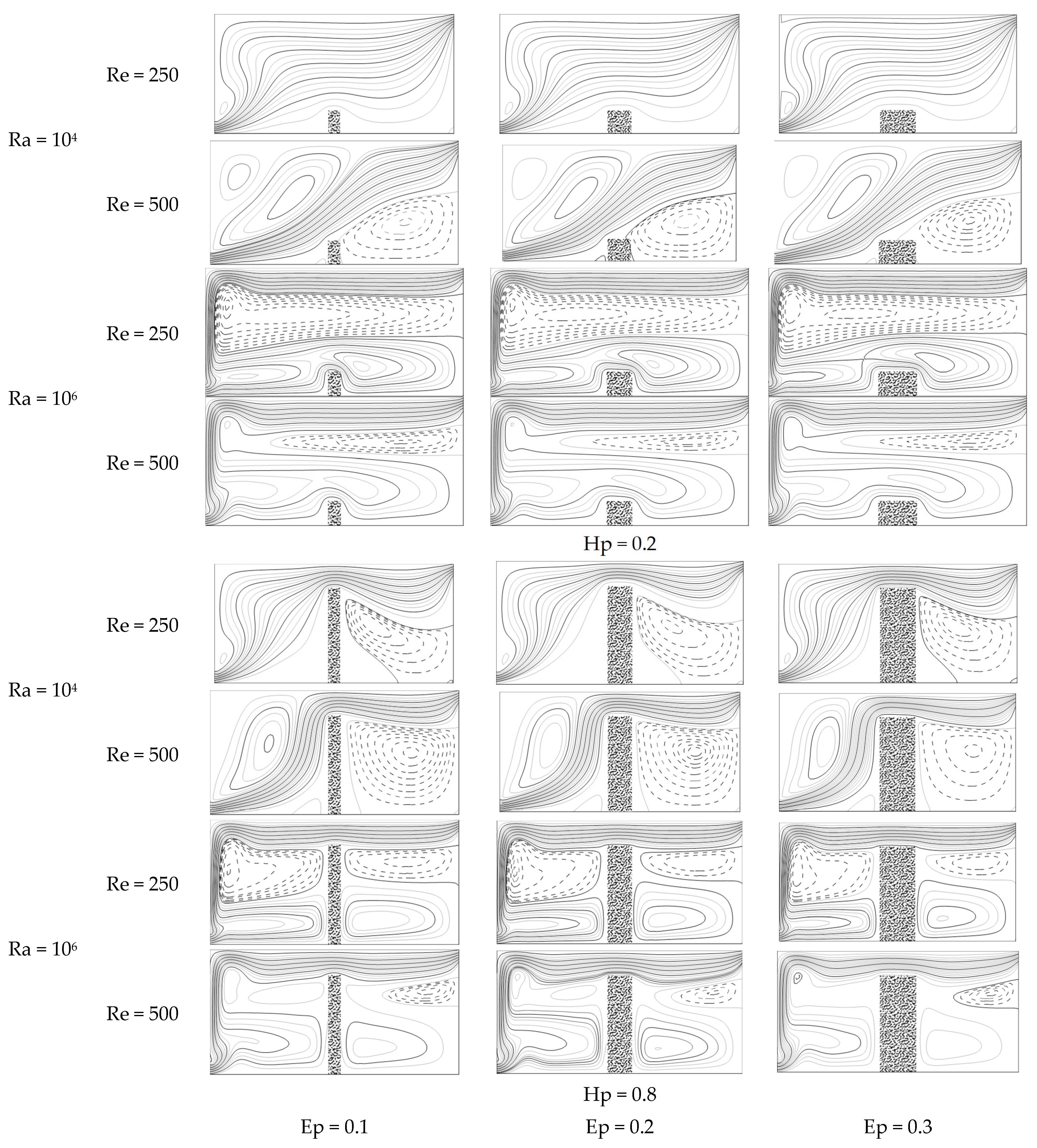
In Figure 4, the stream functions are represented for two thicknesses of porous medium (Ep = 0.1 and 0.3) with a scan of two Reynolds numbers (Re = 250 and Re = 500). In this figure also, we find the illustrations of the figures related to two Darcy numbers (Da = 10⁻⁴ and 10⁻⁶) as well as three Rayleigh numbers, which give us the sweep of the range Ra [10²–10⁶]. We observe in this figure that the thickness of the porous wall preserves the same principle of general flow movement, mainly with three combined movements. With a jet of fresh fluid coming from the inlet port, the last bypasses the porous medium, sometimes to the outlet and other times to the active wall for large Reynolds values. Note that the porous wall thickness has very little influence on the flow, and its effect is only visible for intermediate permeabilities (Da = 10⁻⁴) wherein the dimension of the recirculation zone of the second compartment is affected.

The influence of the porous medium height is illustrated in Figure 5 for the two heights considered (Hp = 0.2 and Hp = 0.8). This figure confirms the relative independence of the flow structures with the porous wall thickness in the considered thickness range Ep ∈ [0.1–0.3]. Note that when the height of the porous wall is important, the second compartment is characterized by at least one recirculation zone for low Rayleigh values. When the thermal draft increases (Ra = 10⁶), a recirculation zone is also obtained in the first compartment of the cavity. When the porous wall is one fifth of the chamber height (Hp = 0.2), the stream functions follow the same path as the fluid regime (Figure 3 for Da = 10⁻²), the only difference being the size of the swirls.

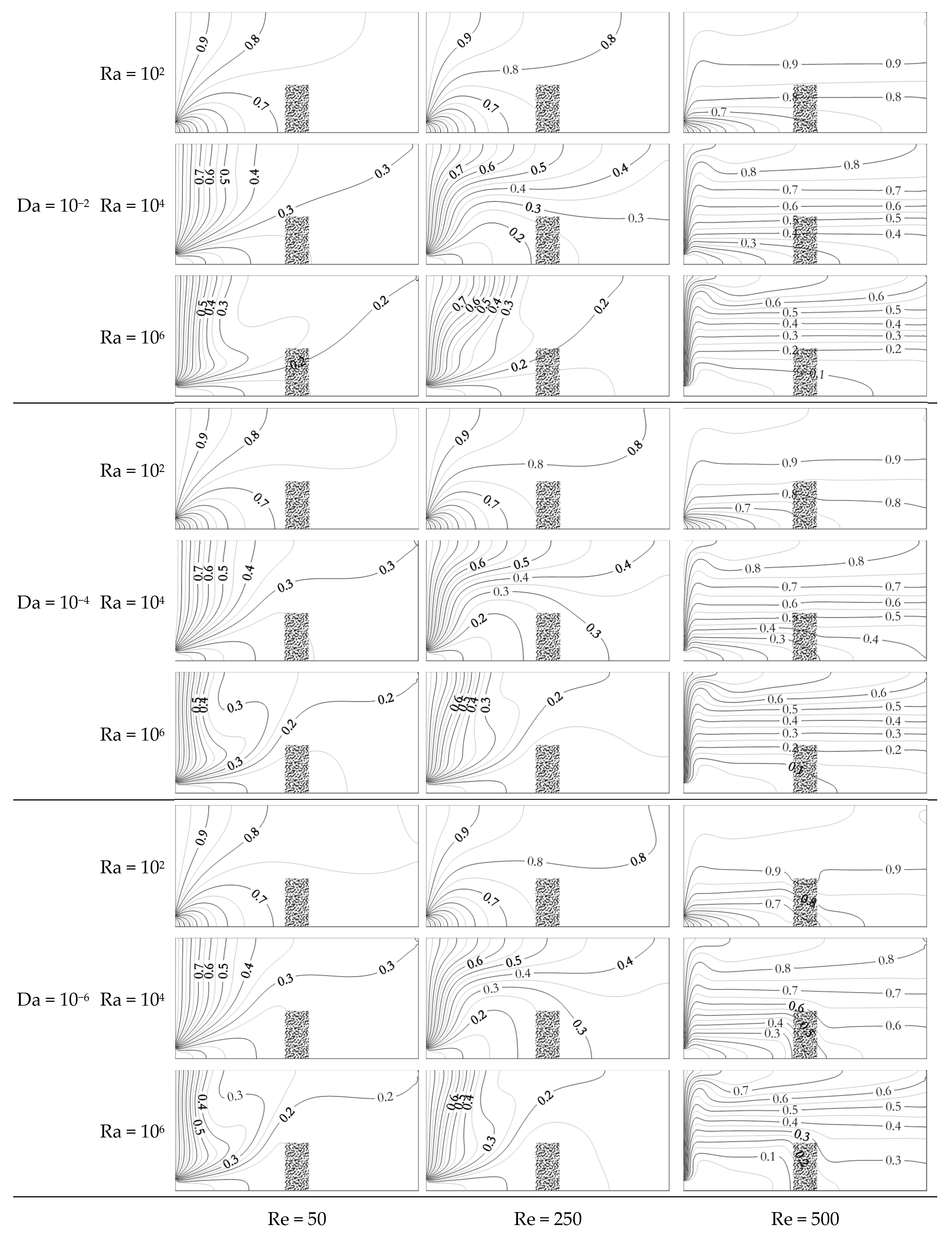
Figure 6, Figure 7 and Figure 8 illustrate isotherms as a function of the control parameters for the same conditions chosen in Figure 3, Figure 4 and Figure 5, respectively. It is noted that the interval between two successive isotherms is constant and is equal to 0.05. It is also mentioned that the dimensionless temperature varies from the minimum value at the inlet (θ = 0) to the maximum value near the active wall (θ = 1). It can be seen from these figures that the porous medium does not offer any resistance to the isotherms, and no distortion is observed. This is probably due to the fact that a unit conductivity ratio has been considered. The most pertinent remark is that the influence of the porous wall thickness is not very visible on the isotherms (confirmed in Figure 8), which may indicate that the Nusselt numbers (on the heat transfer figures) will be independent of the porous wall thickness.

In Figure 6, we notice that for large values of Darcy number (i.e., Da = 10⁻²), the increase in Rayleigh number changes isotherms from a distributed form (fan-shaped) to vertical lines stuck at the hot wall. When Re increases, we show a flattening of the thermal boundary layer, probably due to the large flow rate of the parietal fluid, which carries more energy. In the left-hand compartment of the cavity, a vertical stratification zone is formed which clearly illustrates the thermal boundary layer. Additionally, in the right compartment, horizontal thermal stratification is observed as the Reynolds number increases. So, isotherms pass from an almost constant temperature between 0.15 and 0.25 to a vertical temperature stratification along a range depending on the Rayleigh number.

For a low-permeability porous partition, Da = 10⁻⁶, it can be seen that the isotherms are not affected except for large Reynolds values where the flow structures are affected by the presence of the porous obstacle.

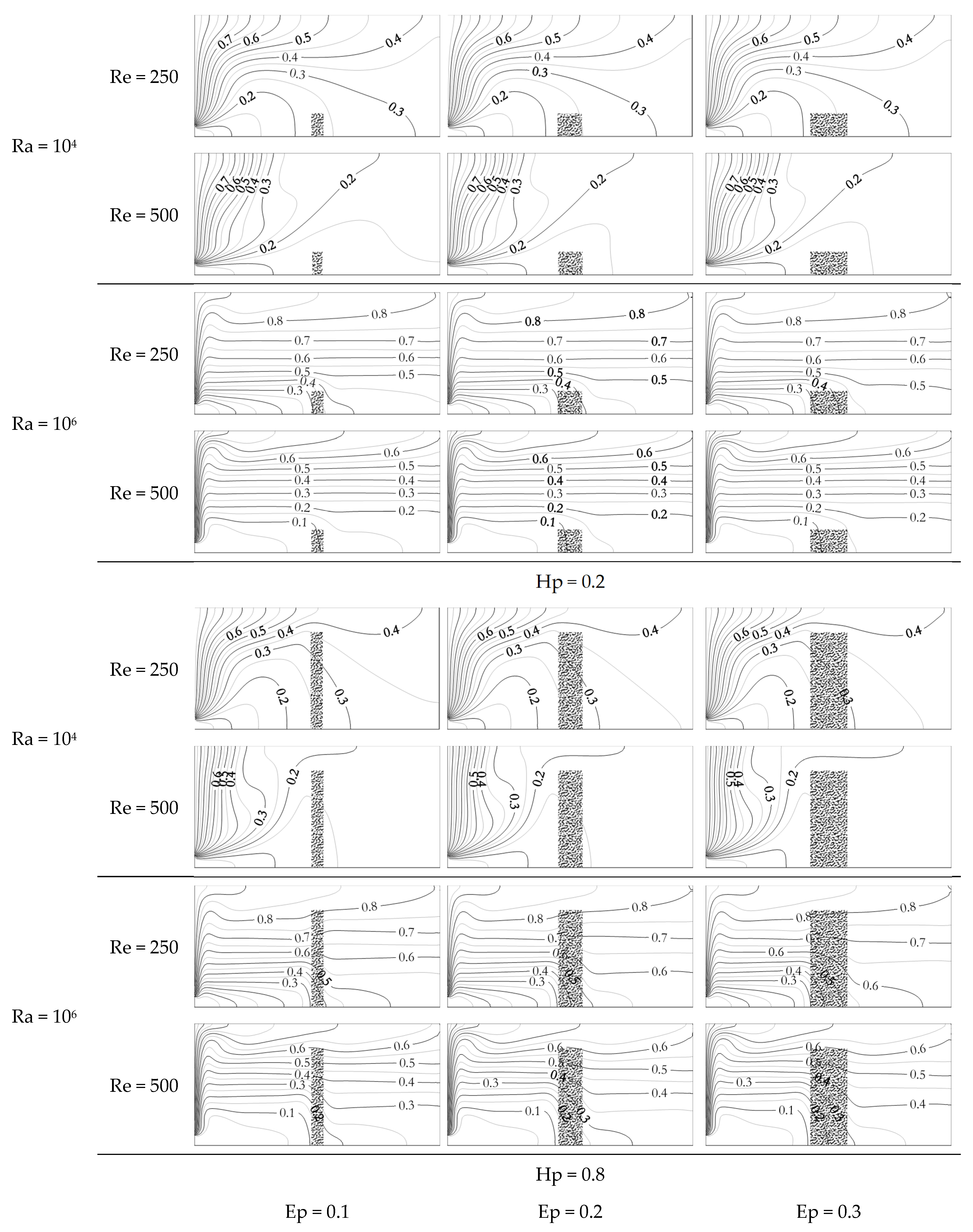
The effect of the thickness and height of the porous wall is illustrated in Figure 8, wherein it can be seen that the partition influences the isotherms in the cavity. This influence is more visible in the second compartment when the thermal draft is the maximum for the maximum height considered (Hp = 0.8). When the height is minimal, no influence is observed.

For average values of the Darcy number (Da = 10⁻²), the increase in Ra gives isotherms passing from a distributed form (aerated) to vertical lines grouped near the hot wall in the form of a thermal boundary layer. With increasing Re, this thermal boundary layer flattens out due to the high fluid flow. In the rest of the cavity (right section), a stratification zone is formed. Subsequently, when the Reynolds number increases, a horizontal thermal stratification is observed, which will give rise to a natural convection motion represented in the graphs of the flow functions. For the porous partition with low permeability (Da = 10⁻⁶), its presence is remarkable because at its level the isotherms lose their horizontal shape going towards Re > 250 and Ra > 10⁴ and the stratification is visible on both sides of the partition with a slight difference in the range of variation that represents larger values in the left space of the cavity.

Figure 9 shows the transfer rate, an expression of the Nusselt number, as a function of the control parameters. On the abscissa axis, we find the Darcy number, which gives us the relative permeability of the porous wall. The different lines on the graph represent the variation in the driving parameters (i.e., Reynolds and Rayleigh numbers) of the problem for two heights of porous media considered (Ep = 0.3, Hp = 0.2 and Hp = 0.8). We can see very well on this figure that when the height of the porous wall is small (Hp = 0.2), its effect is negligible on the heat transfer and the curves have almost horizontal linear lines depending only on the intensities of the two natural and mechanical motors (i.e., Rayleigh and Reynolds numbers). This is certainly due to the fact that when the height of the porous wall is equal to 20% of the height of the chamber, its effect remains local and influences the transfers very little. It is shown in this figure that the heat transfer is directly dependent on the Rayleigh and Reynolds numbers.

When the height is the maximum (Hp = 0.8, on Figure 8), the heat transfer increases with a reduction in the permeability, but its influence remains weak (less than 10% increase). This can be explained by the fact that for low Darcy numbers, the flow is disturbed by a solid obstacle generating vortices that swirl the inner fluid, thus favoring heat transfer. Note that for the case of a porous partition height of 80%, we are in the presence of an optimization situation wherein an intermediate Reynolds of Re = 250 gives us the maximum heat transfer.

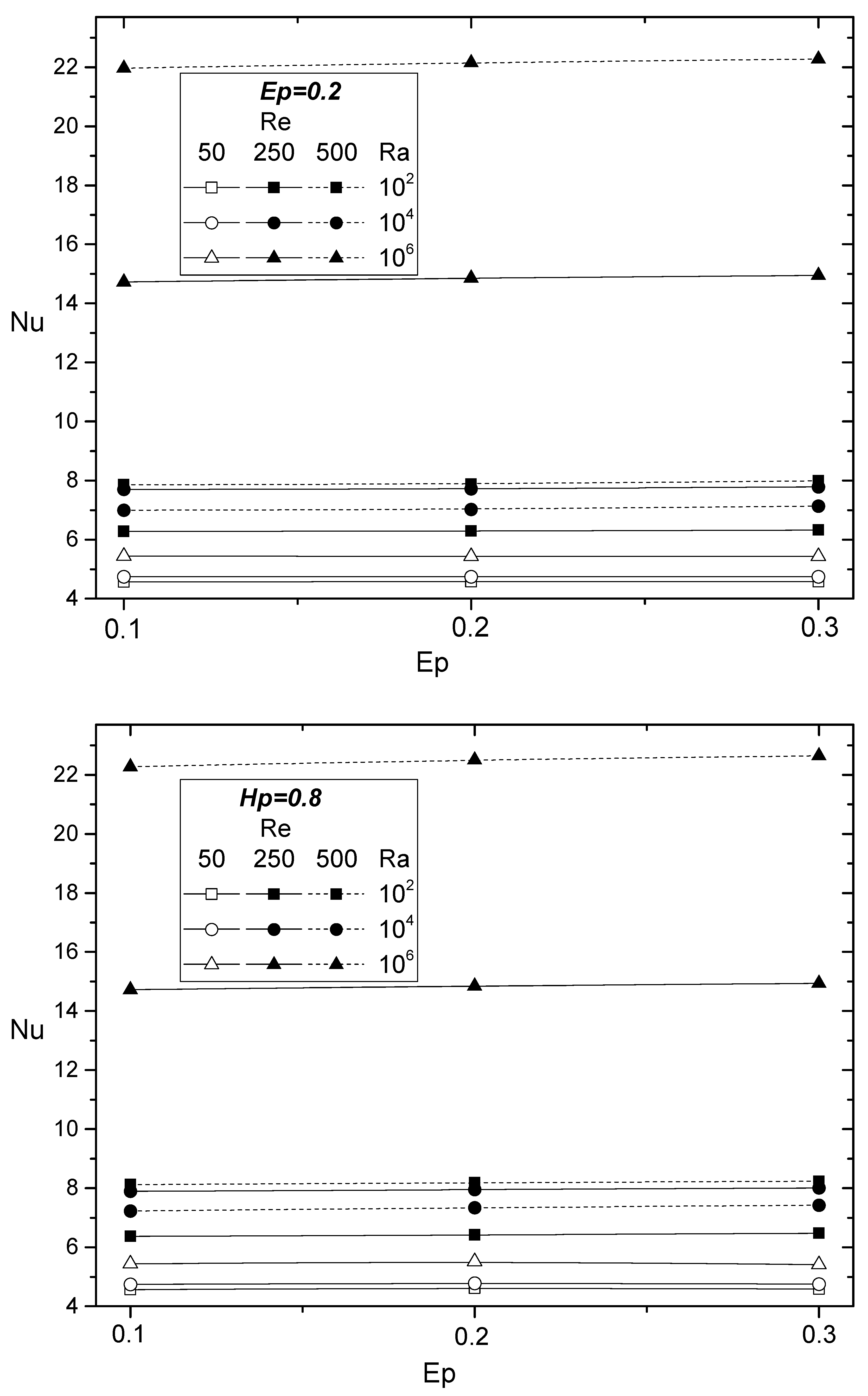
Figure 10 shows the results of numerical simulations of the heat transfer rate (Nusselt number) as a function of the geometric dimensions of the porous wall (Hp and Ep, respectively, height and thickness) and for the driving parameters of the ventilation system (i.e., Reynolds and Rayleigh numbers). Note that, in this figure, we have considered the case of a porous medium with low permeability (Da = 10⁻⁶). The shape of the curves is slightly increasing linearly, for the Rayleigh of large values, depending on the thickness of the porous wall for the height Hp = 0.8. This is due to the fact that, in this situation, the fluid is constricted in the first compartment and then directed towards the active wall, thus increasing the heat transfer. For the other Rayleigh cases, the increase in transfer is not visible and the plots show an almost horizontal linear trend. Note that optimization cases are found wherein a larger heat transfer is obtained for intermediate Reynolds numbers; (Re,Ra) = (250,10⁺⁶) gives a larger heat transfer than (500,10⁺⁶).

For the natural convection case (Ra = 10⁶), the evolution of the Nusselt number is increasing linearly with the Darcy number on a log–log scale. Note that the effect of the porous medium (permeability, height, and thickness) is not remarkable, with the same result for the behavior of the curves, which tend to join.

The analysis of the heat transfer rate (Nusselt number) in the case of forced convection shows that it increases as the Reynolds number increases. This is obvious since the fluid is attracted to the heated wall (see graphs of the stream function), thus increasing the flow through the hot wall and subsequently causing an intensive extraction of hot fluid.

6. Conclusions

The flow structures and heat transfer have been numerically analyzed in a displacement-ventilated chamber. The conservation equations have been written by adopting some simplifying assumptions and then solved by the lattice Boltzmann method. The numerical results of the developed computational code have been compared with those of the literature. The findings of our research are quite convincing; thus, the following conclusions can be drawn:

• The flow structures are complex and dependent on the control parameters where we find the spatial competition between a fluid jet of forced convection and the acceleration by natural convection at the hot wall;
• When the permeability of the porous wall is high (Da = 10⁻²), the porous wall offers no resistance, which can be defined as a fluid regime;
• When the permeability of the porous wall is very small (Da = 10⁻⁶), the porous wall behaves like a solid in this limit of the Darcien regime;
• The porous wall has very little influence on the heat transfer, but its dimensions and permeability influence the temperature field, mainly in the second compartment;
• The elevation of the separation thickness does not significantly change the curves evolution of the Nusselt number according to Ra and Re. The differences between these curves for different porous separation thickness are reduced, and the maximum values obtained for Re = 500 and Ra = 10⁶.