Reducing the Deterioration of Sentiment Analysis Results Due to the Time Impact ^†

Abstract

The research identifies and substantiates the problem of quality deterioration in the sentiment classification of text collections identical in composition and characteristics, but staggered over time. It is shown that the quality of sentiment classification can drop up to 15% in terms of the F-measure over a year and a half. This paper presents three different approaches to improving text classification by sentiment in continuously-updated text collections in Russian: using a weighing scheme with linear computational complexity, adding lexicons of emotional vocabulary to the feature space and distributed word representation. All methods are compared, and it is shown which method is most applicable in certain cases. Experiments comparing the methods on sufficiently representative text collections are described. It is shown that suggested approaches could reduce the deterioration of sentiment classification results for collections staggered over time.

1. Introduction

Automated knowledge mining and text analysis have raised much interest in both scientific and practical aspects. The interest is driven by Internet users who publish hundreds of thousands opinions on social networks, blogs, forums and specialized portals every day; data that require complete processing. This explains the high demand for the systems of automated sentiment detection and opinion mining among the professionals involved in the development of recommendation and expert systems, marketing experts and analysts providing marketing research, political experts evaluating the tonality of news and public sentiments, among other experts.

Automatic sentiment text classification is a rather topical subject. Microblog posts are usually short and do not exceed 300 characters, which allows us to consider that their classification takes place at the phrase or sentence level. Classification at the level of short phrases and expressions, rather than entire documents or paragraphs [1,2], has been carried out by Wilson, Wiebe and Hoffmann [3]. In their paper, the authors showed that it is important to determine the sentiment (positive or negative) of a single sentence, not the whole text in its entirety. As for a long document, the author’s opinion about an issue can change from positive to negative and vice versa. In addition, the author may speak negatively about minor shortcomings, but overall retain a positive attitude regarding the subject described in the text. In other words, a long document or review cannot always be clearly classified as positive or negative in sentiment. Despite the fact that microblogging is quite a young phenomenon, researchers are actively involved in analyzing the tonality of blog posts, in general, and tweets, in particular [4,5,6,7].

Microblog posts are short enough to describe all the different aspects of a product or service and, at the same time, are full of opinions and emotional assessments, so short-text sentiment classification is dealt with not only on the phrase and sentence level, but also relative to the stated subject [8,9].

One of the challenges in developing and using a sentiment analysis system is that their performance constantly deteriorates over time. This occurs mainly due to the fact that active vocabulary is constantly expanding with new terms, as well as with the emotionally-colored ones and thus requires regular updates of sentiment lexicons.

However, the idea of this paper is to compare suggested approaches among themselves, to show the pros and cons of each approach and to suggest the conditions of suitable use. It is important to mention that all collections are domain independent and written in Russian. Furthermore, a detailed description of the methods is given so they that can be reproduced.

This paper is an extended and improved version of [10], and the following new sections and information are added:

• a section about the third method of “weighting scheme with linear computational complexity”;
• a section about the “metrics of the classifier’s performance evaluation”;
• extended information about collection gathering and preprocessing;
• added information about five sentiment lexicons based on the training collection;
• as well as some figures and tables, which can help to understand the data.

Some minor updates are given within the text.

The study is organized as follows: The second section identifies and substantiates the problem of quality deterioration in the sentiment classification of text collections identical in composition and characteristics, but staggered over time. In this regard, the collections on which experiments were conducted are described, as well as the measures for assessing the quality of the results. The results of experiments regarding the classifier’s performance for text collections collected 6–18 months apart are given. The third section proposes an approach to solving this problem. The final section consists of the findings and a conclusion.

2. Reduced Quality of Sentiment Classification Due to Changes in Emotional Vocabulary

Social networks’ users are among the first to use new terms in everyday life. The 40 new words added to the Oxford Dictionary in 2013 included terms from social networks, such as “srsly” and “selfie”. The active vocabulary is constantly updated; therefore, automatic classifiers must take this into account in their models. When it comes to machine learning, the the training collection of texts must be expanded. In the context of rules and dictionaries, it is necessary to take into account the slang that social networks are saturated with in order to improve the quality of classifiers.

2.1. Short Text Collections

Studies and experiments with automatic text classification show that the results of classification usually depend on the training text sample and the subject area to which the training collection corresponds. Today, many projects center on feature engineering and the involvement of additional data, such as external text collections (that do not overlap with the training collection) or sentiment lexicons. Additional information can reduce the reliance on the training collection and improve the classification results.

In order to successfully build the sentiment classifier for the text collection, it is necessary to have text collections tagged by sentiment. Moreover, in order to improve sentiment classification in dynamically-updated collections, it is necessary to have several text collections, compiled in different periods of time.

The first corpus was collected between December 2013 and February 2014. For the sake of brevity, we shall call it the “I_collection ”. Using the method [11] and filtration [12] proposed by the author, a training collection was formed from the I_collection texts.

Next, it is necessary to collect and prepare the test text collections. The second corpus, which consists of about 10 million short texts, was collected during July–August 2014. The third corpus consisting of about 20 million texts was compiled in July and November 2015.

Two test collections were formed from the 2014 and 2015 texts (“II_collection” and “III_collection”, respectively). Both text collection have undergone the same filtration as the training I_collection. Test collections have been distributed by different sentiment classes using the same method [11] as for the training collection. The distribution of texts in the collections by sentiment class is presented in

Table 1. Distribution of texts in the collections by sentiment class.

	Positive Messages	Negative Messages	Neutral Messages
I_collection	114,911	111,922	107,990
II_collection	5000	5000	4293
III_collection	10,000	10,000	9595

. All three collections were domain-independent, i.e., they do not belong to any predefined subject area.

All experiments were performed on Russian text collections. Texts containing both positive and negative emotions were deleted from the collection. Such texts cannot be automatically attributed to either collection of posts (positive or negative). Uninformative tweets (less than 40 characters long) were deleted. It was previously shown by the author [4] that the collections were complete and sufficiently representative.

The compiled text collections formed the basis for the training and test collections of Twitter posts used to assess the sentiments of tweets towards a given subject at the classifier competition SentiRuEval [9,13,14] in 2015 and 2016.

2.2. Metrics of Classifier’s Performance Evaluation

In order to evaluate performance of a sentiment classifier system, the results obtained by an automated classifier system are compared to the reference tagged ones. Based on the difference between the reference values and the results obtained for the collection automatically tagged by the algorithm to be evaluated, the following common metrics were calculated: accuracy (Formula (1)), precision (Formula (2)), recall (Formula (3)) and F-measure (Formula (4)) [15].

$$Accuracy=\frac{(TP+TN)}{(TP+FP+TN+FN)}$$

(1)

Precision is the fraction of objects classified as X that actually belong to the X class, or the probability that a randomly-chosen tweet is classified as relevant to the class to which it actually belongs (Formula (2)).

$$Precision=\frac{TP}{(TP+FP)}$$

(2)

Recall is the fraction of all objects of the X class that are classified by the algorithm as relevant to the X class, or the probability that a tweet randomly chosen from a class will be classified as relevant to this particular class (Formula (3)).

$$Recall=\frac{TP}{(TP+FN)}$$

(3)

In this paper, the F-measure is calculated as the mean of F-measures of all the tonality classes. Similarly, precision and recall are calculated as mean values of the precision and recall values of all the individual tonality classes:

$$F-measure=2\times \frac{Precision\times Recall}{Precision+Recall}$$

(4)

where $TP$ is a true positive decision, the number of texts correctly assigned to the class i by the automatic classificator; $FP$ is the false positive decision, the number of texts that are not correctly assigned to the class i; $FN$ is the false negative decision, the number of texts that are not correctly assigned to the class i; $TN$ is the true negative decision, the number of texts correctly assigned to the class i.

2.3. The Problem of Reduced Quality in Sentiment Classification Due to Changes in Emotional Vocabulary

To simulate a real-life situation, when language or the topics discussed on social media may change over time, a second and third collection of short texts were prepared. The first and the second collections were compiled about six months apart, the first and the third a year and a half. At first glance, it would seem that vocabulary cannot change so quickly; however, the topics of tweets, which affect the overall mood in general and reputation in particular, are significantly dependent on positive or negative events that occur involving the target; usually, such events cannot be predicted in advance. For example, in January and February 2014, about 12% of all tweets were about the Olympics, whereas in August 2014, mentions of the Olympic Games did not exceed 0.5% of all posts.

First, it is necessary to show the decrease in classification quality for collections staggered over time. To do this, we will train the classifier model on the I_collection and apply it to the II_collection and III_collection. The lexicons men_3, men_5 and BOW were selected to build a feature space. The men_N prefix indicates that a term is found no less than N times in one of the collections that corresponds to a sentiment class (positive, negative or neutral). The total quantity of terms in the training collection was designated as BOW (bag-of-words).

The experiment results that show the reduction in quality of text classification are presented in

Table 2. Quality measurements for the classification of microblog posts by sentiment for collections staggered over time.

BOW				Men_3_TF-IDF				Men_5_TF-IDF
Acc	P	R	F	Acc	P	R	F	Acc	P	R	F
I_collection
0.7459	0.7595	0.7471	0.7505	0.6457	0.6591	0.6471	0.6506	0.6189	0.6542	0.6184	0.6223
II_collection
0.6964	0.6984	0.7062	0.6933	0.5086	0.5829	0.5040	0.5026	0.5745	0.5823	0.5795	0.5808
III_collection
0.6118	0.6317	0.6156	0.5996	0.4651	0.5218	0.4638	0.4549	0.5343	0.5337	0.5360	0.5344

. Table 2 shows that over a year and a half, the classification quality of microblog texts can fall to 15–20% according up to the F-measure, depending on the selected set of features.

3. Ways to Reduce the Deterioration of Classification Results for Text Collections Staggered over Time

The SVM (support vector machine) method and LIBLINEAR library [16] were used as the classifier. The LIBLINEAR library is an implementation of the SVM algorithm with a linear kernel. Experiments show that the LIBLINEAR library significantly surpasses its counterparts in speed when training a model, so it was used for this paper with the basic parameters.

3.1. Weighting Scheme with Linear Computational Complexity

Active vocabulary is constantly expanding with new words and expressions. The first method to prevent the vocabulary from becoming obsolete is to update it regularly. This allows us to detect new terms appearing in the language and to take them into account in sentiment classification. However, regular updates of the vocabulary and recalculation of weights assigned to its terms are rather computational complexity. Thus, the idea is to find a weighting scheme for the regular updates that requires less computing power. For example, in order to use a method based on the TF-IDF measure, we need to know term frequency in collections; thus, the dataset should remain unchanged during the weight calculation. This significantly complicates the calculations required for vocabulary update if the calculations should be performed in real time. Every piece of new information updates the vocabulary, so when a new text is added to a collection, it is necessary to recalculate the weights for all the terms in the collection. The computational complexity of the weight recalculation for all terms of the collection is $O\left(N^2\right)$. The problem of finding and calculating the weights of terms in real time is solved by means of term frequency–inverse corpus frequency (TF-ICF) (Formula (5)) [17].

$$TF-ICF=tf\times log(1+\frac{\left|C\right|}{cf\left(t_i\right)})$$

(5)

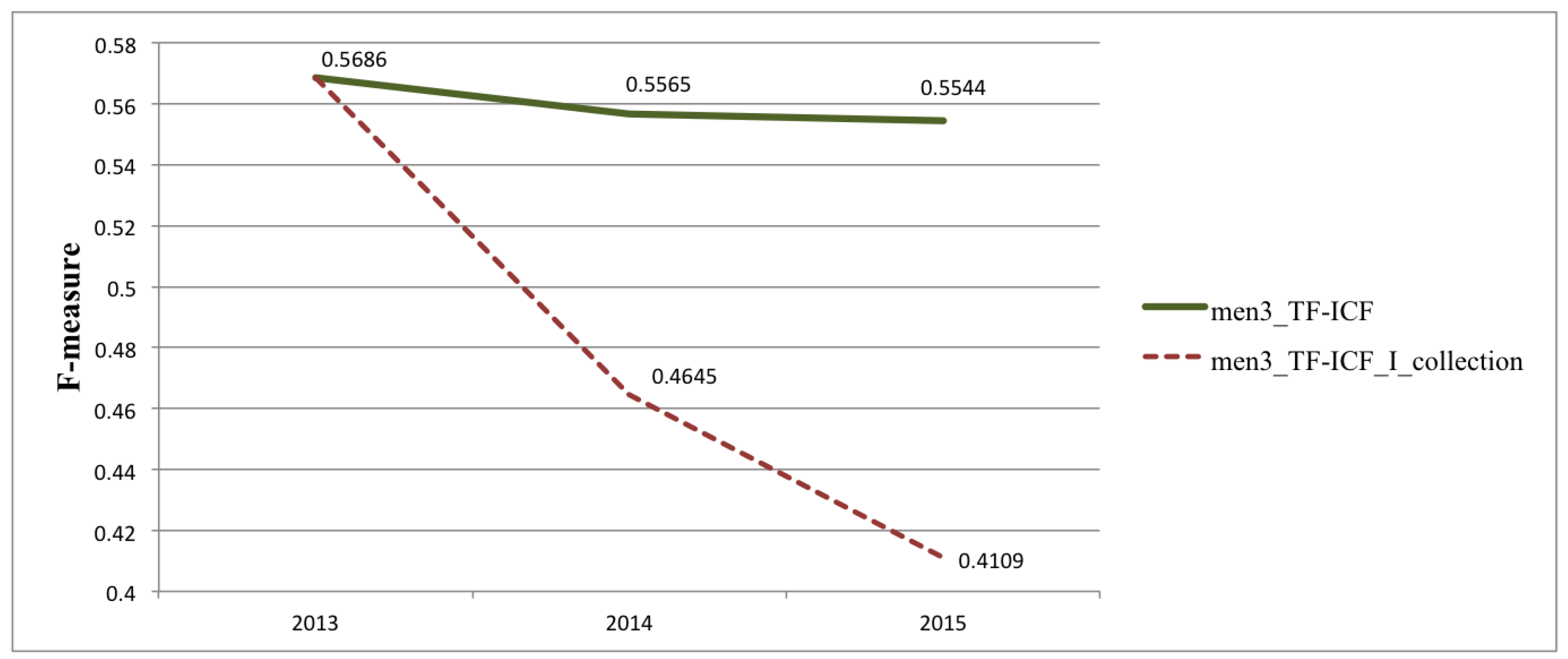
In this formula, C is the number of categories and $cf$ is the number of categories that include the term to be weighted. TF-ICF does not require any information on the frequency of a term in other documents of the collection; it only needs to know the category to which the term belongs; thus, the computational complexity of $ICF$ is $O\left(N\right)$. The next step is to validate if TF-ICF can be used to weigh features for sentiment text classification. First of all, it is necessary to obtain the basic values of classifier’s results that we need to improve. In order to do this, a vocabulary from the I_collection was created. Then, the vocabulary as a base for the feature vector space was used. The TF-ICF measure was used to weigh the features of the vector model text representation. Furthermore, a Boolean model was employed (a feature may take only one of two values: 0, absent; 1, present). The I_collection was used as the training set, and a classifier model was created based on it. The II_ and III_collections were used as the test sets. In order to choose features, an experiment with vocabularies of TF-ICF-weighed terms was set up. Figure 1 shows the classifier’s results according to the F-measure. The figure reveals that when terms from vocabularies that are met in one of the sentiment collections less than three times (men_3) and less than five times (men_5) were deleted, the vocabularies showed the best results. Furthermore terms that were met in the entire training collection less than 1, 3 and 5 times were deleted from the vocabularies 1_0_0, 3_0_0 and 5_0_0 respectively. Figure 1 shows the value of the F-measure in cross-validation with the training collection for every vocabulary with TF-ICF measured features depending on the feature vector space.

It is obvious that the men_3_icf and men_5_icf vocabularies show the best classifier’s results according to the F-measure in the cross-validation with the I_collection; therefore, they were used to test the resulting model of the classifier on the II_ and III_ collections.

Table 3. F-measure and accuracy sentiment classification with two TF-ICF-weighed lexicons.

	Men_3_TF-ICF		Men_5_TF-ICF
	F-Measure	Accuracy	F-Measure	Accuracy
I_collection	0.5686	0.5648	0.5526	0.5541
II_collection	0.4645	0.4833	0.4564	0.4971
III_collection	0.4109	0.4278	0.4143	0.4516

shows the F-measure results while applying the model to the II_ and III_collections. For clarity, we preserve the F-measure values in the cross-validation with the I_collection.

When the classifier is tested on collections from different periods, the quality of its performance is decrease. According to the F-measure, the classification quality can fall up to 15%. Although the TF-ICF weighing scheme has shortcomings, such as a relatively low F-measure, the scheme also has a significant advantage (linear computational complexity), which is especially important when being applied to a vector space containing hundreds of thousands of features. The next step is to merge the I_collection vocabulary with the II_collection vocabulary, recalculate the weights for the resulting vocabulary, use it to create a classifier based on the I + II joint collection and test it on the III_collection. The F-measure for cross-validation of the classifier built on the men_3_TF-ICF feature vocabulary is expected to be in the proximity of 0.5686 (see Table 3), and the F-measure for the III collection is expected to exceed 0.4109. Some experiments have also been done with the BOW feature vocabulary. The classifier performance according to the F-measure is provided in

Table 4. Performance of the classifier with the I + II joint collection added to the training collection.

	BOW				Men_3_TF-ICF
	Acc	P	R	F	Acc	P	R	F
I + II cross-validation	0.7205	0.7339	0.7215	0.7250	0.5539	0.5806	0.5550	0.5565
III_collection	0.6848	0.6889	0.6862	0.6872	0.5348	0.5571	0.5361	0.5334

.

The classifier does show a better F-measure for the III collection in both cases—for the men_3_TF-ICF vocabulary and for the bag-of-words method—while maintaining the results of the classifier’s cross-validation with the training collection at the level of 0.55–0.57 for men_3_TF-ICF (Table 3) and at the level of 0.72–0.75 for the bag-of-words (Table 4). As the third step, all three collections were merged into one. Just as in the previous experiment, the goal of the classifier is to keep the resulting level no lower than 0.55 according to the F-measure for the men_3_TF-ICF feature vocabulary and no lower than 0.72 for the bag-of-words. The classifier performance for the I_, II_ and III_ joint collection is shown in Figure 2. Figure 2 conveniently illustrates that dynamic lexicon updates allow us to limit the decrease in quality of sentiment classification for collections from different periods. The solid line shows F-measures for updates of the vocabulary and the training collection, and the dashed line marks the classification results obtained when the I_ collection was used as a training set.

The classifier showed a uniform performance in all the experiments and thus allowed us to judge the results’ validity.

The accumulation of large amounts of text makes the use of TF-IDF for dynamic recalculation of the term’s weights in real time more difficult. In the case of the bag-of-words method, the vocabulary size (and thus, the dimension of the feature vector) will be constantly increasing, consuming more computing power without increasing the quality of classification, which is kept at the level of 0.72–0.75 according to the F-measure. The use of a filtered vocabulary and TF-ICF helps to retard the increase of the feature vectors’ dimension and allow the terms’ weights to be calculated in real time, but the quality of the classification remains at 0.55 according to the F-measure. The use of the method described above is justified when the computing power is limited and there are no external sentiment vocabularies and additional text collections.

3.2. Using External Lexicons of Emotional Words and Expressions

The second hypothesis is that the use of external lexicons with emotive and/or evaluative vocabulary will improve the quality of text classification by tonality, as well as reducing the classifier’s dependency on the training collection. The terms in the lexicon can be used as features in machine learning [18] or as part of approaches based on dictionaries and rules [19]. There have been studies describing the derivation and configuration of sentiment lexicons on a certain predetermined subject area [20,21]. Examples are given of terms that can describe positive features in one subject area, but neutral or even negative ones in another. However, according to [18,22], combining training data from different domains improves the quality of sentiment classification in each of the selected subject areas. Consequently, there are many evaluative words with a strongly-pronounced tonal orientation that are suitable for different subject areas.

Two general-topic lexicons of emotional language, tagged by experts, were used as additional external dictionaries for this paper: RuSentiLex and Linis-crowd.

RuSentiLex [23] is a lexicon compiled from several sources: evaluative words from Russian thesaurus RuTez, slang words from Twitter and words with positive or negative associations (connotations) from a news corpus. The lexicon contains more than ten thousand words and phrases in the Russian language. It includes emotional terms automatically extracted from text and checked by experts.

Another dictionary used in this paper is Linis-crowd [24]. Despite the fact that the authors used socio-politically-themed texts to form the lexicon, it is noted that the dictionary contains vocabulary that is not specific to this subject area, but conveys an emotional assessment, which is why the authors of the dictionary decided to include it in the Linis-crowd prototype. The dictionary contains 9539 terms. Each one is weighted from −2 (strongly negative) to +2 (strongly positive).

Activation of sentiment lexicons: For a sentiment classifier based on machine learning methods, lexicon features were added in addition to features generated on the basis of training data. For each term w in the lexicon with polarity p, a value (w, p) was determined:

$$(w,p)=\left\{\begin{array}{cc}>0,\hfill & w-positive\hfill \\ <0,\hfill & w-negative\hfill \\ =0,\hfill & w-neutral\hfill \end{array}\right.$$

The following were added as features:

• The total number of terms (w, p) in the text of the tweet;
• The sum of all polarity values of words in the lexicon: ${\sum }_{w\in tweet}(w,p)$;
• The maximum polarity value: ${\max }_{w\in tweet}(w,p)$.

Each of the lexicons was activated separately, and comparison of their performance can be seen in

Table 5. Classifier results while activating lexicons RuSentiLex and Linis-crowd.

	RuSentiLex				Linis-Crowd
	Acc	P	R	F	Acc	P	R	F
2013	0.7273	0.74	0.7284	0.7318	0.7272	0.7398	0.7283	0.7316
2014	0.7245	0.7387	0.7259	0.7295	0.7244	0.7386	0.7258	0.7294
2015	0.6724	0.6802	0.6733	0.6759	0.6725	0.6803	0.6733	0.6760

. As can be seen from the table, both lexicons show quite similar results when used on the training and test collections.

Consequently, external lexicons made it possible to stop the loss in quality when classifying collections staggered over time. Since the main features were generated by the training collection, the trend towards degradation nevertheless persisted. However, it was reduced from 15% when using the bag-of-words Table 2 to 5.6% when activating emotional vocabulary lexicons.

Clearly, it makes sense to use this method when external sentiment lexicons are available, as it inhibits the reduction in quality when sentiment classifying collections are staggered over time.

3.3. Using Distributed Word Representations as Features

In the previous methods, the feature space for training the classifier was based on the training collection and was therefore highly dependent on the quality and completeness of this collection. Despite the good results of the models described above, there were no semantic relationships between the terms, and the continuous addition of new terms led to an increase in the dimension of the feature vector space. Another way to overcome the obsolescence of lexicon is the use of the distributed word representations as features to train the classifier.

3.3.1. The Space of Distributed Word Representations

Distributed word representation (word embedding) is a k-dimensional feature vector $w=(w_1,\dots ,w_k)$, where $w_i\in R$ is the vector coordinate [25]. When compared with the Boolean or other weighted vector models, the number of coordinates k of such a vector is much smaller. Usually, this number does not exceed several hundred, whereas in the Boolean model, it is measured in tens of thousands, depending on the original size of the lexicon.

In addition to reducing feature vector length, distributed word representation takes into account the meaning of a word in context. In other words, it allows us to extend “fast car”, for example, into “speedy automobile”, which is absent in the training sample, thereby reducing dependence on the latter.

Unsupervised machine learning models are used to obtain distributed word representations, for instance, CBOW, Skip-Gram, AdaGram [26] and Glove. Recent studies showed [27] that the neural language model Skip-Gram is superior to others in the quality of obtained vector representations. Therefore, the Skip-Gram model was used in this paper.

3.3.2. Using the Skip-Gram Model to Reduce Dependence on the Training Collection

The Skip-Gram model was proposed by Thomas Mikolov et al. in 2013 [28]. An untagged corpus of texts is input into the model, and the number of occurrences in the corpus is calculated for each word. An array of words is sorted by frequency, and rare words are removed. As a rule, you can set a threshold to consider all words, which are met fewer times than specified in the threshold, as rare and delete them.

It is shown in [29] that neural networks using vector representations of words obtained by means of the word2vec algorithm [26] can effectively solve the problem of natural language text processing in general, and of text classification by sentiment in particular. This algorithm has shown the best results on the selected text collections in comparison to others.

In order to train the Skip-Gram model, five million texts were arbitrarily selected from the original I_collection, not split into sentiment classes. The II_ and III_ collections did not take part in training, since it was assumed that the trained model should be transferable to later collections.

Word2Vec [26] was used as a software implementation of the Skip-Gram model with the following parameters:

• size 300: every word is represented as a vector of this length;
• windows 5: how many words of context the training algorithm should take into account;
• negative 10: the number of negative examples for negative sampling;
• samples 1 × 10⁻⁴: sub-sampling (the usage of sub-sampling improves performance); the recommended parameter for sub-sampling is from 1 × 10⁻³–1 × 10⁻⁵;
• threads 10: the number of threads to use;
• min-counts 3: limits the size of the lexicon to significant words. Words that appear in the text less than this specified number of times were ignored; the default value was five;
• iter 15: the amount of training iterations.

Emoticons were filtered out of the text, as they designate that a text belongs to a particular sentiment class as emoticons used for the distinct supervision.

Each text is represented as an averaged vector of its constituent words (Formula (6)):

$$d=\frac{\sum w_i}{n}$$

(6)

where $w_i$ is the vector representation of the its word in the studied text and i = (1, …, n); n is the number of unique words from the lexicon found in the analyzed text.

The classifier was trained on the I_collection, and then, the trained classifier model was used to test the II_ and III_ collections. The classifier results are shown in

Table 6. The results of sentiment classification with the aid of vectors obtained by using Word2Vec as features.

	Acc.	Precision	Recall	F-Measure
I_collection	0.7206	0.7250	0.7221	0.7226
II_collection	0.7756	0.7763	0.7836	0.7787
III_collection	0.7289	0.7250	0.7317	0.7252

; the quality measurements for the I_collection are given for clarity.

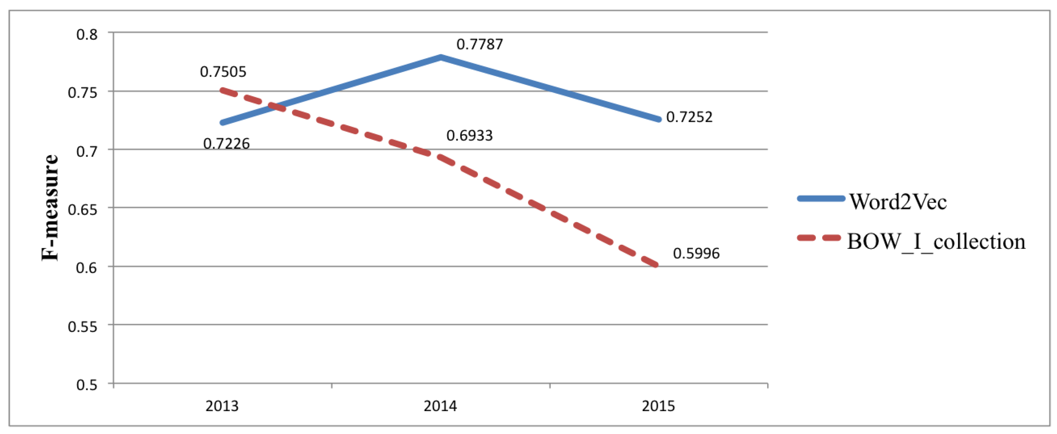
Figure 3 clearly demonstrates that the quality of classification into three classes is not reduced for collections complied 6–12 months apart and remains at the level of the best values obtained using the bag-of-words model when cross-validating on a collection from one year (Table 2 and Table 4). Nevertheless, the number of coordinates in the word vector is exactly 300 (according to the settings), rather than exceeding 200,000, like in the Boolean or vector models.

This method is well suited for use in the event that we have an external, fairly representative collection of texts, which is similar in vocabulary to the training and test collections, meaning that here, as for other neural networks, a large training sample of texts is required. This method makes it possible to obtain stable and consistent results for text classification by sentiment.

4. Conclusions

This paper suggests three fundamentally different models to overcome the deterioration of sentiment classification results for collections staggered over time. In Table 2, it was shown that the quality of text classification by sentiment can be reduced to 15% according to the F-measure over 18 months. Therefore, the aim of the approaches proposed in this paper is to minimize the decrease in quality when classifying text collections that are staggered over time.

(1) The first approach supposes using a weighing scheme with linear computational complexity. Thus, it enables one to update the lexicon dynamically and retrain the classifier. This approach has a weaker dependence on the training collection because the training collection is constantly updating. In this case, the difference between the classifier’s performance on the I_ and III_ collections is only 2.4% according to the F-measure for the bag-of-words methods and 1.42% for TF-ICF. Regardless of its apparent advantages, the approach has two shortcomings:

• Updating the lexicon increases the dimension of the feature space. Thus, with every lexicon update, the system requires more resources, and the text vector becomes more sparse.
• The quality of classification with TF-ICF is significantly lower than with the bag-of-words method.

(2) The second approach is based on adding lexicons of emotional vocabulary: RuSentiLex and Linis-crowd. The use of external dictionaries makes it possible to reduce the gap in classification quality between the I_ and III_ collections to 5.6%, according to the F-measure. The difference between the classification results of the I_ and II_ is less than 1%; only 0.2%. At the same time, the quality of the classifier remains at the 0.68–0.73 level, which is comparable with the best results. Therefore, the generation of features based on external lexicons does not entail a large increase in the feature space and makes it possible to achieve good classification results. Despite this, since the feature space is still dependent on a training collection, there is a negligible reduction in classification quality for later collections.

(3) The foundation of the third approach is the concept of a distributed word representation space and the Skip-Gram neural language model. As in the second approach, external resources were used here. The distributed word representation space was built on an untagged collection of tweets that was many times larger than the automatically-tagged training collection. The averaged word vectors from one tweet were used as features. Thus, the length of the vector space was only 300; this is the first advantage of the approach. A second advantage of the approach is the classification results: the difference between the I_ and III_collection according to the F-measure is 0.26%, with the classification results for the III_collection being higher. The classification results of the I_ and II_ collections are similar: the II_collection sets exceed the I_collection values by 5.6%, according to the F-measure. This can be explained by the fact that a cross-validation method was used on the I_collection, i.e., the collection was divided into training and test sets at a ratio of 4:5, whereas the full I_collection was used to train the classifier for testing on the II_ and III_ collections.

In summary, all three proposed approaches can reduce the deterioration of sentiment classification results for collections staggered over time.

References

1. Pang, B.; Lee, L. Thumbs up? Sentiment classification using machine learning techniques. In Proceedings of the Conference on Empirical Methods in Natural Language Processing (EMNLP), Philadelphia, PA, USA, 6–7 July 2002; pp. 79–86. [Google Scholar]
2. Turney, P. Thumbs up or thumbs down? Semantic orientation applied to unsupervised classification of reviews. In Proceedings of the 40th Annual Meeting of the Association for Computational Linguistics (ACL-02), Philadelphia, PA, USA, 7–12 July 2002; Association for Computational Linguistics: Philadelphia, PA, USA, 2002; pp. 417–424. [Google Scholar]
3. Wilson, T.; Wiebe, J.; Hoffmann, P. Recognizing contextual polarity in phrase level sentiment analysis. In Proceedings of the Human Languages Technologies Conference/Conference on Emperical Methods in Natural Language Processing (HLT/EMNLP 2005), Vancouver, BC, Canada, 5–8 October 2005. [Google Scholar]
4. Rubtsova, Y.V. Research and Development of Domain Independent Sentiment Classifier. Trudy SPIIRAN 2014, 36, 59–77. [Google Scholar] [CrossRef]
5. Agarwal, A.; Xie, B.; Vovsha, I.; Rambow, O.; Passonneau, R. Sentiment analysis of twit-ter data. In Proceedings of the Workshop on Languages in Social Media, Portland, OR, USA, 23 June 2011; Association for Computational Linguistics: Stroudsburg, PA, USA, 2011; pp. 30–38. [Google Scholar]
6. Kouloumpis, E.; Wilson, T.; Moore, J. Twitter sentiment analysis: The good the bad and the omg! In Proceedings of the Fifth International AAAI Conference on Weblogs and Social Media, Barcelona, Spain, 17–21 July 2011; Volume 11, pp. 538–541. [Google Scholar]
7. Pak, A.; Paroubek, P. Twitter as a Corpus for Sentiment Analysis and Opinion Mining. In Proceedings of the Seventh International Conference on Language Resources and Evaluation, Valletta, Malta, 17–23 May 2010; Volume 10, pp. 1320–1326. [Google Scholar]
8. Lek, H.H.; Poo, D.C.C. Aspect-based Twitter sentiment classification. In Proceedings of the 2013 IEEE 25th International Conference on Tools with Artificial Intelligence, Herndon, VA, USA, 4–6 November 2013; pp. 366–373. [Google Scholar]
9. Loukachevitch, N.; Rubtsova, Y. Entity-Oriented Sentiment Analysis of Tweets: Results and Problems. In Proceedings of the International Conference on Text, Speech, and Dialogue, Pilsen, Czech Republic, 14–17 September 2015; Springer International Publishing: Cham, Switzerland, 2015; pp. 551–559. [Google Scholar]
10. Rubtsova, Y. Reducing the Degradation of Sentiment Analysis for Text Collections Spread over a Period of Time. In Proceedings of the International Conference on Knowledge Engineering and the Semantic Web, Szczecin, Poland, 8–10 November 2017; Springer: Cham, Switzerland, 2017; pp. 3–13. [Google Scholar]
11. Read, J. Using emoticons to reduce dependency in machine learning techniques for sen-timent classification. In Proceedings of the 43rd Meeting of the Association for Computational Linguistics (ACL-05), Ann Arbor, MI, USA, 25–30 June 2005; Association for Computational Linguistics: Stroudsburg, PA, USA, 2005. [Google Scholar]
12. Rubtsova, Y.V. A Method for development and analysis of short text corpus for the review classiification task. In Proceedings of the XV All-Russian Scientific Conference “Digital libraries: Advanced Methods and Technologies, Digital Collections” (RCDL2013), Yaroslavl, Russia, 14–17 October 2013; pp. 269–275. [Google Scholar]
13. Loukachevitch, N.; Rubtsova, Y. Entity-Oriented Sentiment Analysis of Tweets: Results and Problems. In Proceedings of the XVII International Conference on Data Analytics and Management in Data Intensive Domains, Obninsk, Russia, 13–16 October 2015; pp. 499–507. [Google Scholar]
14. Loukachevitch, N.; Rubtsova, Y. SentiRuEval-2016: Overcoming Time Gap and Data Sparsity in Tweet Sentiment Analysis. In Computational Linguistics and Intellectual Technologies, Proceedings of the International Conference on “Dialogue 2016”, Moscow, Russia, 1–4 June 2016; Association for Computational Linguistics: Stroudsburg, PA, USA, 2016; pp. 375–384. [Google Scholar]
15. Manning, C.D.; Schutze, H. Foundations of Statistical Natural Language Processing; The MIT Press: Cambridge, MA, USA, 1999. [Google Scholar]
16. Fan, R.-E.; Chang, K.-W.; Hsieh, C.-J.; Wang, X.-R.; Lin, C.-J. LIBLINEAR: A Library for Large Linear Classification. J. Mach. Learn. Res. 2008, 9, 1871–1874. [Google Scholar]
17. Reed, J.W.; Jiao, Y.; Potok, T.E.; Klump, B.A.; Elmore, M.T.; Hurson, A.R. TF-ICF: A New Term Weighting Scheme for Clustering Dynamic Data Streams. In Proceedings of the 2006 5th International Conference on Machine Learning and Applications, Orlando, FL, USA, 14–16 December 2006; pp. 258–263. [Google Scholar]
18. Mohammad, S.M.; Kiritchenko, S.; Zhu, X. NRC-Canada: Build-ing the state-of-the-art in sentiment analysis of tweets. In Proceedings of the Second Joint Conference on Lexical and Computational Semantics (SEMSTAR’13), Atlanta, GA, USA, 13–14 June 2013. [Google Scholar]
19. Taboada, M.; Brooke, J.; Tofiloski, M.; Voll, K.; Stede, M. Lexicon-based methods for sentiment analysis. Comput. Linguist. 2011, 37, 267–307. [Google Scholar] [CrossRef]
20. Klekovkina, M.V.; Kotelnikov, E.V. The automatic sentiment text classification method based on emotional vocabulary. In Proceedings of the 14th All-Russian Scientific Conference “Digital libraries: Advanced Methods and Technologies, Digital Collections”, Pereslavl-Zalessky, Russia, 15–18 October 2012; pp. 118–123. [Google Scholar]
21. Loukachevitch, N.V.; Chetverkin, I.I. Extraction and use of evaluation words in the problem of classifying reviews into three classes. Comput. Methods Programm. 2011, 12, 73–81. [Google Scholar]
22. Mansour, R.; Refaei, N.; Gamon, M.; Abdul-Hamid, A.; Sami, K. Revisiting the Old Kitchen Sink: Do We Need Sentiment Domain Adaptation? In Proceedings of the International Conference Recent Advances in Natural Language Processing (RANLP-2013), Hissar, Bulgaria, 7–13 September 2013; pp. 420–427. [Google Scholar]
23. Loukachevitch, N.V.; Levchik, A.V. Creating a General Russian Sentiment Lexicon. In Proceedings of the Tenth International Conference on Language Resources and Evaluation (LREC 2016), Portoroz, Slovenia, 23–28 May 2016; European Language Resources Association (ELRA): Paris, France, 2016. [Google Scholar]
24. Alexeeva, S.; Koltsov, S.; Koltsova, O. Linis-crowd.org: A lexical resource for Russian sentiment analysis of social media. In Proceedings of the Internet and Modern Society (IMS-2015), Moscow, Russia, 23–25 June 2015; pp. 25–32. [Google Scholar]
25. Titov, I.; McDonald, R. Modeling Online Reviews with Multi-grain Topic Models. In Proceedings of the 17th International Conference on World Wide Web (WWW’08), Beijing, China, 21–25 April 2008; pp. 111–120. [Google Scholar]
26. Mikolov, T.; Sutskever, I.; Chen, K.; Corrado, G.S.; Dean, J. Distributed Representations of Words and Phrases and their Compositionality. In Advances in Neural Information Processing Systems; NIPS: La Jolla, CA, USA, 2013; pp. 3111–3119. [Google Scholar]
27. Levy, O.; Goldberg, Y.; Dagan, I. Improving Distributional Similarity with Lessons Learned from Word Em-bedding. Trans. Assoc. Comput. Linguist. 2015, 3, 211–225. [Google Scholar]
28. Mikolov, T.; Chen, K.; Corrado, G.; Dean, J. Efficient estimation of word representations in vector space. arXiv, 2013; arXiv:1301.3781. [Google Scholar]
29. Kim, Y. Convolutional neural networks for sentence classification. arXiv, 2014; arXiv:1408.5882. [Google Scholar]
Figure 1. The value of the F-measure in the cross-validation with the training collection for every vocabulary with TF-ICF measured features.
Information 09 00184 g001
Figure 2. F-measure with dynamic updates of the lexicon of the training collection (solid line) and without (dash Line).
Information 09 00184 g002
Figure 3. Comparison of the use of model Word2Vec word vectors as features and a lexicon based on a bag-of-words from the I_collection.
Information 09 00184 g003