A Quick Algorithm for Binary Discernibility Matrix Simplification using Deterministic Finite Automata

Abstract

The binary discernibility matrix, originally introduced by Felix and Ushio, is a binary matrix representation for storing discernible attributes that can distinguish different objects in decision systems. It is an effective approach for feature selection, knowledge representation and uncertainty reasoning. An original binary discernibility matrix usually contains redundant objects and attributes. These redundant objects and attributes may deteriorate the performance of feature selection and knowledge acquisition. To overcome this shortcoming, row relations and column relations in a binary discernibility matrix are defined in this paper. To compare the relationships of different rows (columns) quickly, we construct deterministic finite automata for a binary discernibility matrix. On this basis, a quick algorithm for binary discernibility matrix simplification using deterministic finite automata (BDMSDFA) is proposed. We make a comparison of BDMR (an algorithm of binary discernibility matrix reduction), IBDMR (an improved algorithm of binary discernibility matrix reduction) and BDMSDFA. Finally, theoretical analyses and experimental results indicate that the algorithm of BDMSDFA is effective and efficient.

1. Introduction

Decision making can be considered as the process of choosing the best alternative from the feasible alternatives. With the development of research, decision making is extended from one attribute to multiple attributes. To solve problems in multiple attribute decision making, various theories such as fuzzy sets, rough sets and utility theory, etc. have been used. Many of significant results [1,2,3,4,5,6,7,8] have been achieved in multiple attribute decision making. Researchers in rough set theory [9] are usually concerned with attribute reduction (or feature selection) problems of multiple attribute decision making. The binary discernibility matrix, proposed by Felix and Ushio [10], is a useful tool for attribute reduction and knowledge acquisition. Recently, many algorithms of attribute reduction based on binary discernibility matrices have been developed [11,12,13]. In 2014, Zhang et al. [14] proposed a binary discernibility matrix for an incomplete information system, and designed a novel algorithm of attribute reduction based on the proposed binary discernibility matrix. In the paper [15], Li et al. developed an attribute reduction algorithm in terms of the improved binary discernibility matrix, and applied the algorithm in customer relationship management. Tiwari et al. [16] developed hardware for a binary discernibility matrix which can be used for attribute reduction and rule acquisition in an information system. Considering mathematical properties of a binary discernibility matrix, Zhi and Miao [17] introduced the so-called binary discernibility matrix reduction (BDMR), which was actually an algorithm for binary discernibility matrix simplification. On the basis of BDMR, two algorithms for attribute reduction and reduction judgement were presented. A binary discernibility matrix with a vertical partition [18] was proposed to deal with big data in attribute reduction. Ren et al. [19] constructed an improved binary discernibility matrix which can be used in an inconsistent information system. Ding et al. [20] discussed several problems about a binary discernibility matrix in an incomplete system. Combining the binary discernibility matrix in an incomplete system, an algorithm of incremental attribute reduction was proposed. In the paper [20], a novel method for calculation of incremental core attribute was introduced firstly. On this basis, an algorithm of attribute reduction was proposed. As is well known that core attributes play a crucial role in heuristic attribute reduction algorithms. Core attributes are computationally expensive in attribute reduction. Hu et al. [21] gave a quick algorithm of the core attribute calculation using a binary discernibility matrix. The computational complexity of the algorithm is $O\left(\right|C\left|\right|U\left|\right)$, where $\left|C\right|$ is the number of condition attributes and $\left|U\right|$ is the number of objects in the universe.

An original binary discernibility matrix usually contains redundant objects and attributes. These redundant objects and attributes may deteriorate the performance of feature selection (attribute reduction) and knowledge acquisition based on binary discernibility matrices. In other words, storing or processing all objects and attributes in an original binary discernibility matrix could be computationally expensive, especially in dealing with large scale data sets with high dimensions. So far, however, few works about the binary discernibility matrix simplification have been investigated. The existing algorithms regarding binary discernibility matrix simplification are time-consuming. To tackle this problem, our works in this paper concern on how to improve the time efficiency of algorithms of binary discernibility matrix simplification. On this purpose, we construct deterministic finite automata in a binary discernibility matrix to compare the relationships of different rows (or columns) quickly. By using deterministic finite automata, we develop a quick algorithm of binary discernibility matrix simplification. Experimental results show that the proposed algorithm is effective and efficient. The contributions of this paper are summarized as follows: First, we define row and column relations which can be used for constructing deterministic finite automata in a binary discernibility matrix. Second, deterministic finite automata in a binary discernibility matrix are proposed to compare the relationships of different rows (or columns) quickly. Third, based on this method, a quick algorithm for binary discernibility matrix simplification (BDMSDFA) is proposed. The proposed method in this paper is meaningful in practical applications. First, by using BDMSDFA, we obtain the simplified binary discernibility matrices quickly. These simplified binary discernibility matrices can significantly improve the efficiency of attribute reduction (feature selection) in decision systems. Second, a binary discernibility matrix without redundant objects and attributes will have the high performance of learning algorithms, and need less space for data storage.

The rest of this paper is structured as follows. We review basic notions about rough set theory in the next section. In Section 3, we propose a general binary discernibility matrix, and define row relations and column relations in a binary discernibility matrix. In Section 4, we develop a quick algorithm for binary discernibility matrix simplification which is called BDMSDFA. Experimental results in Section 5 show that the algorithm of BDMSDFA is effective and efficient, it can be applicable to simplification of large-scale binary discernibility matrices. Finally, the whole paper is summarized in Section 6.

2. Preliminaries

Basic notions about rough set theory are briefly reviewed in this section. Some further details about rough set theory can be found in the paper [9]. A Pawlak decision system can be regarded as an original information system with decision attributes which give decision classes for objects.

A Pawlak decision system [9] can be denoted by 4-tuple $DS=(U,AT,V,f)$, where universe $U=\{x_1,x_2,\dots ,x_{\left|U\right|}\}$ is a finite non-empty set of objects; attribute set $AT=C\cup D$, $C\cap D=\varnothing$, where $C=\{a_1,a_2,\dots ,a_{\left|C\right|}\}$ is called a condition attribute set and $D=\left\{d\right\}$ is called a decision attribute set in a decision system; $V_{a_m}$ is the domain of a condition attribute $a_m\in AT$, $V={\cup }_{a_m\in AT}{V}_{a_m}$ and $f:U\times AT\to V$ is a function such that $f(x_i,a_m)=a_m\left(x_i\right)\in V_{a_m\in AT}$, $f(x_i,d)=d\left(x_i\right)\in V_{d\in AT}$, where $x_i\in U$.

Given a Pawlak decision system $DS=(U,C\cup D,V,f)$, for $\forall x_i,x_j\in U$, an indiscernibility relation regarding attribute set $B\subseteq C$ is defined as $IND\left(B\right)=\{(x_i,x_j):\forall b\in B,f(x_i,b)=f(x_j,b)\}$. Therefore, the discernibility relation regarding attribute set $B\subseteq C$ is given by $DIS\left(B\right)=\{(x_i,x_j):\exists b\in B,f(x_i,b)\ne f(x_j,b)\}$. The indiscernibility relation regarding $B\subseteq C$ is reflexive, symmetric and transitive. Meanwhile, the discernibility relation is irreflexive, symmetric, but not transitive. A partition of U derived from $IND\left(B\right)$ is denoted by $U/IND\left(B\right)$. The equivalence class in $U/IND\left(B\right)$ containing object $x_i$ is defined as ${\left[x_i\right]}_{IND\left(B\right)}={\left[x_i\right]}_B=\{x_j\in U:(x_i,x_j)\in IND\left(B\right)\}$.

For $\forall B\subseteq C$, the relative indiscernibility relation and discernibility relation with respect to decision attribute set [9] are defined by:

$$IND\left(B\right|D)=\{(x_i,x_j):x_i,x_j\in U,(\forall b\in B\to (f(x_i,b)=f(x_j,b))\vee (f(x_i,d)=f(x_j,d))\},$$

$$DIS\left(B\right|D)=\{(x_i,x_j):x_i,x_j\in U,(\exists b\in B\to (f(x_i,b)\ne f(x_j,b))\wedge (f(x_i,d)\ne f(x_j,d))\}.$$

A relative indiscernibility relation $IND\left(B\right|D)$ with respect to $B\subseteq C$ is reflexive, symmetric, but not transitive. A relative discernibility relation $DIS\left(B\right|D)$ with respect to $B\subseteq C$ is irreflexive, symmetric, but not transitive.

A discernibility matrix, proposed by Skowron and Rauszer [22], suggests a matrix representation for storing condition attribute sets which can discern objects in the universe. Discernibility matrix is an effective method in reduct construction, data representation and rough logic reasoning, and it is also useful mathematical tool in data mining, machine learning, etc. Many extended models of dicernibility matrices have been studied in recent years [23,24,25,26,27,28,29,30]. Considering the classification property $\Delta$, Miao et al. [31] constructed a general discernibility matrix $M_{\Delta }=\left(m_{\Delta }(x_i,x_j)\right)$, where $m_{\Delta }(x_i,x_j)$ is denoted by:

$$m_{\Delta }(x_i,x_j)=\left\{\begin{array}{cc}\{a\in C:f(x_i,a)\ne f(x_j,a)\},& (x_i,x_j)\in DI{S}_{\Delta }\left(C\right|D)\\ \varnothing & \mathrm{otherwise}\end{array},\right.$$

where $(x_i,x_j)\in DI{S}_{\Delta }\left(C\right|D)$ denotes objects $x_i$ and $x_j$ are discernible with respect to the classification property $\Delta$ in a decision system $DS$. It should be noted that $\Delta$ is a general definition on classification property. A general discernibility matrix provides a common solution to attribute reduction algorithms based on discernibility matrices. By constructing different discernibility matrices, the relative attribute reducts with different reduction targets can be obtained. Based on the relative discernibility relation $DIS\left(C\right|D)$, Miao et al. [31] introduced a relationship preservation discernibility matrix which can be denoted as follows:

Definition 1.

[31] Let $DS=(U,C\cup D,V,f)$ be a decision system, for $\forall x_i,x_j\in U$, $\forall a\in C$, $1\le i<j\le \left|U\right|$, $M_{relationship}=\left(m_{relationship}(x_i,x_j)\right)$ is a relationship preservation discernibility matrix, where $m_{relationship}(x_i,x_j)$ is defined by:

$$m_{relationship}(x_i,x_j)=\left\{\begin{array}{cc}\{a\in C:f(x_i,a)\ne f(x_j,a)\}& (x_i,x_j)\in DIS\left(C\right|D)\\ \varnothing & otherwise\end{array}.\right.$$

3. Binary Discernibility Matrices and Their Simplifications

The binary discernibility matrix, initiated by Felix and Ushio [10], is a binary presentation of original discernibility matrix. In this section, we suggest a general binary discernibility matrix. Relations of row pairs and column pairs are discussed respectively. Formally, a binary discernibility matrix [10] is introduced as follows:

Definition 2.

[10] Given a decision system $DS=(U,C\cup D,V,f)$, for $\forall x_i,x_j\in U$ and $\forall a_m\in C$. $M_{BDM}=\left(m_{BDM}(x_i,x_j)\right)$ is a binary discernibility matrix, where the element $m_{BDM}(x_i,x_j)$ is denoted by:

$$m_{BDM}(x_i,x_j)=\left\{\begin{array}{cc}1& f(x_i,a_m)\ne f(x_j,a_m)\wedge d\left(x_i\right)\ne d\left(x_j\right)\\ 0& otherwise\end{array}.\right.$$

Based on a binary discernibility matrix, discernible attributes about $x_i$ and $x_j$ can be easily obtained. A binary discernibility matrix brings us an understandable approach for representations of discernible attributes, and can be used for designing reduction algorithms. To satisfy more application requirements, we extend original binary discernibility matrix to general binary discernibility matrix as follows:

Definition 3.

Given a decision system $DS=(U,C\cup D,V,f)$, for $\forall x_i,x_j\in U$, $\forall a_m\in C$, $M_{BDM}^{\Delta }=\left(m_{BDM}^{\Delta }(x_i,x_j)\right)$ regarding Δ is a general binary discernibility matrix, in which $m_{BDM}^{\Delta }(x_i,x_j)$ is defined by:

$$m_{BDM}^{\Delta }(x_i,x_j)=\left\{\begin{array}{cc}1& (x_i,x_j)\in DI{S}_{\Delta }\left(C\right|D)\\ 0& otherwise\end{array}.\right.$$

$DI{S}_{\Delta }\left(C\right|D)$ is the discernibility relation regarding classification property Δ. The set of rows in $M_{{}_{BDM}}^{\Delta }$ is presented by $R=\{r_1,r_2,\dots ,r_{\left|R\right|}\}$, where $\left|R\right|=\left(\right|U|\times (\left|U\right|-1\left)\right)/2$. The set of columns in $M_{{}_{BDM}}^{\Delta }$ is presented by $C=\{a_1,a_2,\dots ,a_{\left|C\right|}\}$, where $\left|C\right|$ is the cardinality of attribute sets in a decision system. For convenience, a general binary discernibility matrix $M_{{}_{BDM}}^{\Delta }=\left(m_{{}_{BDM}}^{\Delta }(x_i,x_j)\right)$ can be also denoted by $M_{{}_{BDM}}^{\Delta }=\left(m_{{}_{BDM}}^{\Delta }(e_p^m,e_q^m)\right)$. For $\forall a_m\in C$, $\forall r_p,r_q\in R$, $e_{{}_P}^m$ is the matrix element at row $r_p$ and column $a_m$ in $M_{{}_{BDM}}^{\Delta }$, and $e_q^m$ is the matrix element at row $r_q$ and column $a_m$ in $M_{{}_{BDM}}^{\Delta }$, where $1\le p<q\le \left(\right|U|\times (\left|U\right|-1\left)\right)/2$, $1\le m\le \left|C\right|$.

Since a general binary discernibility matrix provides a common structure of binary discernibility matrices in rough set theory, one can construct a binary discernibility matrix according to a given classification property. Any binary discernibility matrix can be also regarded as the special case of the general binary discernibility matrix. Therefore, a general definition of binary discernibility matrix is necessary and important. Based on the relative discernibility relation with respect to D, Definition 2 can be also rewritten as follows:

Definition 4.

Given a decision system $DS=(U,C\cup D,V,f)$, for $\forall x_i,x_j\in U$, $\forall a_m\in C$, $DIS\left(C\right|D)$ is the relative discernibility relation with respect to a condition attribute set C. $M_{BDM}=\left(m_{BDM}(x_i,x_j)\right)$ is a binary discernibility matrix, in which the element $m_{BDM}(x_i,x_j)$ is denoted by:

$$m_{BDM}(x_i,x_j)=\left\{\begin{array}{cc}1& (x_i,x_j)\in DIS\left(C\right|D)\\ 0& otherwise\end{array}.\right.$$

This definition is equivalent to Definition 2 [10]. It is noted that we calculate binary discernibility matrix in this paper by using the relationship preservation discernibility matrix.

Definition 5.

For $\forall a_m\in C$, $\forall r_p,r_q\in R$, $e_{{}_P}^m$ and $e_q^m$ are elements in a binary discernibility matrix $M_{{}_{BDM}}^{}=\left(m_{BDM}(x_i,x_j)\right)$, a row pair with respect to attribute $a_m$ is denoted by $<e_p^m,e_q^m>\in$ {< 0,0 >, < 0,1 >, < 1,0 >, < 1,1 >}, a binary relation between row $r_p$ and $r_q$ is defined as $R_{row}=\{<e_p^m,e_q^m>:1\le p<q\le \left|R\right|\}$.

Similar to Definition 5, we define a column pair and a binary relation with respect to columns as follows.

Definition 6.

For $\forall a_m,a_n\in C$, $\forall r_p\in R$, elements $e_{{}_P}^m$ and $e_p^n$ in a binary discernibility matrix $M_{{}_{BDM}}^{}=\left(m_{BDM}(x_i,x_j)\right)$, a column pair with respect to row $r_p$ is denoted by $<e_p^m,e_p^n>\in${ < 0,0 >, < 0,1 >, < 1,0 >, < 1,1 >}, a binary relation between column $a_m$ and $a_n$ is defined as $R_{col}=\{<e_p^m,e_p^n>:1\le m<n\le \left|C\right|\}$.

For the matrix element $e_p^m$ and $e_q^m$ in the same column $a_m$, we define three row relations in a binary discernibility matrix as follows.

Definition 7.

Given a binary discernibility matrix $M_{{}_{BDM}}^{}=\left(m_{BDM}(x_i,x_j)\right)$, $\forall r_p,r_q\in R$,

(1) 

for $\forall a_m\in C$, $\exists a_n\in C$, $r_p\supset r_q$ if and only if $e_p^m+e_q^m=e_p^m$ and $e_p^n\ne e_q^n$; for $\forall a_m\in C$, $\exists a_n\in C$, $r_q\supset r_p$ if and only if $e_q^m+e_p^m=e_q^m$ and $e_q^n\ne e_p^n$;

(2) 

for $\forall a_m\in C$, $r_p=r_q$ if and only if $e_p^m=e_q^m$;

(3) 

for $\exists a_m,a_n\in C$, $r_p\ne r_q$ if and only if $e_p^m+e_q^m=e_q^m(e_p^m\ne e_q^m)$ and $e_p^n+e_q^n=e_p^n$ $(e_p^n\ne e_q^n)$.

Analogous to Definition 7, for matrix elements $e_p^m$ and $e_p^n$ in the same row $r_p$, we define column relations in a binary discernibility matrix as follows.

Definition 8.

Given a binary discernibility matrix $M_{{}_{BDM}}^{}=\left(m_{BDM}(x_i,x_j)\right)$, $\forall a_m,a_n\in C$,

(1) 

for $\forall r_p\in R$, $\exists r_q\in R$, $a_m\supset a_n$ if and only if $e_p^m+e_p^n=e_p^m$ and $e_q^m\ne e_q^n$; for $\forall r_p\in R$, $\exists r_q\in R$, $a_n\supset a_m$ if and only if $e_p^n+e_p^m=e_p^n$ and $e_q^n\ne e_q^m$;

(2) 

for $\forall r_p\in R$, $a_m=a_n$ if and only if $e_p^m=e_p^n$;

(3) 

for $\exists r_p,r_q\in R$, $a_m\ne a_n$ if and only if $e_p^m+e_p^n=e_p^m(e_p^m\ne e_p^n)$ and $e_q^m+e_q^n=e_q^n$$(e_q^m\ne e_q^n)$.

Let $A_p$ be the elements’ set of a prime implicant in a disjunctive normal form with row $r_p$ and $A_q$ be the elements’ set of a prime implicant in a disjunctive normal form with row $r_q$, then $r_p\supset r_q$ means that $A_p$ is the superset of $A_q$. For $\forall a_m,a_n\in C$, $a_m\supset a_n$ indicates attribute $a_m$ can distinguish more objects in the universe. In a binary discernibility matrix, the row in which all elements are 0s indicates there are no attribute can discern the related objects, and the column in which all elements are 0s indicates that this attribute cannot discern objects in the universe.

In [17], Zhi and Miao first proposed an algorithm of a binary discernibility matrix simplification shown in Algorithm 1. To improve the efficiency of BDMR, Wang et al. [32] introduced an improved algorithm of binary discernibility matrix reduction shown in Algorithm 2.

Algorithm 1: An algorithm of binary discernibility matrix reduction, BDMR.

Input: Original binary discernibility matrix $M_{BDM}$;

Output: Simplified binary discernibility matrix $M_{BDM}^{{}^{\prime }}$

1: delete the row in which all elements are 0 s; 2: for$p=1$to$\left|R\right|$do 3:     for $q=1$ to $\left|R\right|$ do 4:         if $r_p\supset r_q$ then 5:            delete row $r_p$ 6:            break 7:         end if 8:     end for 9: end for 10: delete the column in which all elements are 0 s; 11: for$m=1$to$\left|C\right|$do 12:     for $n=1$ to $\left|C\right|$ do 13:         if $a_n\supset a_m$ then 14:            delete column $a_m$ 15:            break 16:         end if 17:     end for 18: end for 19: output a simplified binary discernibility matrix $M_{BDM}^{\prime }$;

Algorithm 2: An improved algorithm of binary discernibility matrix reduction, IBDMR.

Input: Original binary discernibility matrix $M_{BDM}$;

Output: Simplified binary discernibility matrix $M_{BDM}^{{}^{\prime }}$

1: delete the row in which all elements are 0 s; 2: sort rows in ascending order by the quantity of the number ‘1’ in each row 3: for$p=1$to$\left|R\right|$do 4:     for $q=1$ to $\left|R\right|$ do 5:         if $r_p\supset r_q$ then 6:            delete row $r_p$ 7:            break 8:         end if 9:     end for 10: end for 11: delete the column in which all elements are 0 s; 12: for$m=1$to$\left|C\right|$do 13:     for $n=1$ to $\left|C\right|$ do 14:         if $a_n\supset a_m$ then 15:            delete column $a_m$ 16:            break 17:         end if 18:     end for 19: end for 20: output a simplified binary discernibility matrix $M_{BDM}^{\prime }$;

4. A Quick Algorithm for Binary Discernibility Matrix Simplification

In this section, we investigate two theorems related to row relations and column relations respectively. Based on the two theorems, deterministic finite automata for row and column relations are introduced. Deterministic finite automata can be carried out to obtain the row relations and column relations quickly. By using deterministic finite automata, we propose an algorithm of binary discernibility matrix simplification using deterministic finite automata (BDMSDFA).

Theorem 1.

Let $M_{BDM}=\left(m_{BDM}(x_i,x_j)\right)$ be a binary discernibility matrix, for $\forall a_m\in C$, $\forall r_p,r_q\in R$, $\left|R\right|=\left(\right|U|\times (\left|U\right|-1\left)\right)/2$, we have:

(1) 

if $r_p\supset r_q$, then there exists $<1,0>\in \{<e_p^m,e_q^m>:1\le p<q\le |R\left|\right\}$;

(2) 

if $r_q\supset r_p$, then there exists $<0,1>\in \{<e_p^m,e_q^m>:1\le p<q\le |R\left|\right\}$;

(3) 

if $r_p=r_q$, then there exists $<0,0>\in \{<e_p^m,e_q^m>:1\le p<q\le |R\left|\right\}$ or

                             $<1,1>\in \{<e_p^m,e_q^m>:1\le p<q\le |R\left|\right\}$;

(4) 

if $r_p\ne r_q$, then there exists $<1,0>\in \{<e_p^m,e_q^m>:1\le p<q\le |R\left|\right\}$ and

                             $<0,1>\in \{<e_p^m,e_q^m>:1\le p<q\le |R\left|\right\}$.

Proof. 

(1)

If there does not exist $<1,0>\in \{<e_p^m,e_q^m>:1\le p<q\le |R\left|\right\}$, then $<0,0>\in \{<e_p^m,e_q^m>:1\le p<q\le |R\left|\right\}$ or $<0,1>\in \{<e_p^m,e_q^m>:1\le p<q\le |R\left|\right\}$ or $<1,1>\in \{<e_p^m,e_q^m>:1\le p<q\le |R\left|\right\}$. We have seven binary relations as follows: $\{<0,0>\}$, $\{<0,1>\}$, $\{<1,1>\}$, $\{<0,0>,<0,1>\}$, $\{<0,0>,<1,1>\}$, $\{<0,1>,<1,1>\}$ and $\{<0,0>,<0,1>,<1,1>\}$. From seven binary relations above, if $\forall a_m\in C$, $\exists a_n\in C$, one cannot get $e_p^m+e_q^m=e_p^m(e_p^n\ne e_q^n)$. Thus, there exists $<1,0>\in \{<e_p^m,e_q^m>:1\le p<q\le |R\left|\right\}$ in $M_{BDM}$.

(2)

If there does not exist $<0,1>\in \{<e_p^m,e_q^m>:1\le p<q\le |R\left|\right\}$, then $<0,0>\in \{<e_p^m,e_q^m>:1\le p<q\le |R\left|\right\}$ or $<1,0>\in \{<e_p^m,e_q^m>:1\le p<q\le |R\left|\right\}$ or $<1,1>\in \{<e_p^m,e_q^m>:1\le p<q\le |R\left|\right\}$. Thus, we can also have seven binary relations as follows: $\{<0,0>\}$, $\{<1,0>\}$, $\{<1,1>\}$, $\{<0,0>,<1,0>\}$, $\{<0,0>,<1,1>\}$, $\{<1,0>,<1,1>\}$ and $\{<0,0>,<1,0>,<1,1>\}$. From seven binary relations above, if $\forall a_m\in C$ and $\exists a_n\in C$, one cannot get $e_p^m+e_q^m=e_q^m(e_q^n\ne e_p^n)$. Thus, there exists $<0,1>\in \{<e_p^m,e_q^m>:1\le p<q\le |R\left|\right\}$ in $M_{BDM}$.

(3)

If there does not exist $<0,0>\in \{<e_p^m,e_q^m>:1\le p<q\le |R\left|\right\}$ or $<1,1>\in \{<e_p^m,e_q^m>:1\le p<q\le |R\left|\right\}$. There must have seven binary relations as follows: $\{<0,1>\}$, $\{<1,0>\}$, $\{<0,1>,<1,0>\}$, $\{<0,0>,<0,1>\}$, $\{<0,0>,<1,0>\}$, $\{<1,1>,<0,1>\}$, $\{<1,1>,<1,0>\}$. From seven binary relations above, we cannot have $e_p^m=e_q^m$. Thus, there exists $<0,0>\in \{<e_p^m,e_q^m>:1\le p<q\le |R\left|\right\}\}$ or $<1,1>\in \{<e_p^m,e_q^m>:1\le p<q\le |R\left|\right\}\}$ in $M_{BDM}$.

(4)

If there does not exist $<1,0>\in \{<e_p^m,e_q^m>:1\le p<q\le |R\left|\right\}$ and $<0,1>\in \{<e_p^m,e_q^m>:1\le p<q\le |R\left|\right\}$. We may obtain eleven binary relations as follows: $\{<0,0>\}$, $\{<1,1>\}$, $\{<0,1>\}$, $\{<1,0>\}$, $\{<0,0>,<0,1>\}$, $\{<0,0>,<1,0>\}$, $\{<1,1>,<0,1>\}$, $\{<1,1>,<1,0>\}$, $\{<0,0>,<1,1>\}$, $\{<0,0>,<1,1>,<0,1>\}$, $\{<0,0>,<1,1>,<1,0>\}$. From eleven binary relations, for $\forall a_m\in C$, we cannot have $e_p^m\ne e_q^m$. Thus, there exists $<1,0>\in \{<e_p^m,e_q^m>:1\le p<q\le |R\left|\right\}$ and $<0,1>\in \{<e_p^m,e_q^m>:1\le p<q\le |R\left|\right\}$ in $M_{BDM}$.

This completes the proof. ☐

Analogous to Theorem 1, we can easily obtain the following theorem as:

Theorem 2.

Let $M_{BDM}=\left(m_{BDM}(x_i,x_j)\right)$ be a binary discernibility matrix, for $\forall a_m,a_n\in C$, $\forall r_p\in R$, we can have:

(1) 

if $a_m\supset a_n$, then there exists $<1,0>\in \{<e_p^m,e_p^n>:1\le m<n\le |C\left|\right\}$;

(2) 

if $a_n\supset a_m$, then there exists $<0,1>\in \{<e_p^m,e_p^n>:1\le m<n\le |C\left|\right\}$;

(3) 

if $a_m=a_n$, then there exists $<0,0>\in \{<e_p^m,e_p^n>:1\le m<n\le |C\left|\right\}$ or

                             $<1,1>\in \{<e_p^m,e_p^n>:1\le m<n\le |C\left|\right\}$;

(4) 

if $a_m\ne a_n$, then there exists $<1,0>\in \{<e_p^m,e_p^n>:1\le m<n\le |C\left|\right\}$ and

                             $<0,1>\in \{<e_p^m,e_p^n>:1\le m<n\le |C\left|\right\}$.

Proof. 

(1)

If there does not exist $<1,0>\in \{<e_p^m,e_p^n>:1\le m<n\le |C\left|\right\}$, then $<0,0>\in \{<e_p^m,e_p^n>:1\le m<n\le |C\left|\right\}$ or $<0,1>\in \{<e_p^m,e_p^n>:1\le m<n\le |C\left|\right\}$ or $<1,1>\in \{<e_p^m,e_p^n>:1\le m<n\le |C\left|\right\}$. We have seven binary relations as follows: $\{<0,0>\}$, $\{<0,1>\}$, $\{<1,1>\}$, $\{<0,0>,<0,1>\}$, $\{<0,0>,<1,1>\}$, $\{<0,1>,<1,1>\}$ and $\{<0,0>,<0,1>,<1,1>\}$. From seven binary relations above, if $\forall r_p\in R$, $\exists r_q\in R$, one cannot get $e_p^m+e_p^n=e_p^m(e_q^m\ne e_q^n)$. Thus, there exists $<1,0>\in \{<e_p^m,e_p^n>:1\le m<n\le |C\left|\right\}$ in $M_{BDM}$.

(2)

If there does not exist $<0,1>\in \{<e_p^m,e_p^n>:1\le m<n\le |C\left|\right\}$, then $<0,0>\in \{<e_p^m,e_p^n>:1\le m<n\le |C\left|\right\}$ or $<1,0>\in \{<e_p^m,e_p^n>:1\le m<n\le |C\left|\right\}$ or $<1,1>\in \{<e_p^m,e_p^n>:1\le m<n\le |C\left|\right\}$. Thus, we can also have seven binary relations as follows: $\{<0,0>\}$, $\{<1,0>\}$, $\{<1,1>\}$, $\{<0,0>,<1,0>\}$, $\{<0,0>,<1,1>\}$, $\{<1,0>,<1,1>\}$ and $\{<0,0>,<1,0>,<1,1>\}$. From seven binary relations above, if $\forall r_p\in R$ and $\exists r_q\in R$, one cannot get $e_p^m+e_p^n=e_p^n(e_q^m\ne e_q^n)$. Thus, there exists $<0,1>\in \{<e_p^m,e_p^n>:1\le m<n\le |C\left|\right\}$ in $M_{BDM}$.

(3)

If there does not exist $<0,0>\in \{<e_p^m,e_p^n>:1\le m<n\le |C\left|\right\}$ or $<1,1>\in \{<e_p^m,e_p^n>:1\le m<n\le |C\left|\right\}$. There must have seven binary relations as follows: $\{<0,1>\}$, $\{<1,0>\}$, $\{<0,1>,<1,0>\}$, $\{<0,0>,<0,1>\}$, $\{<0,0>,<1,0>\}$, $\{<1,1>,<0,1>\}$, $\{<1,1>,<1,0>\}$. From seven binary relations above, we cannot have $e_p^m=e_p^n$. Thus, there must exists $<0,0>\in \{<e_p^m,e_p^n>:1\le m<n\le |C\left|\right\}$ or $<1,1>\in \{<e_p^m,e_p^n>:1\le m<n\le |C\left|\right\}$ in $M_{BDM}$.

(4)

If there does not exist $<1,0>\in \{<e_p^m,e_p^n>:1\le m<n\le |C\left|\right\}$ and $<0,1>\in \{<e_p^m,e_p^n>:1\le m<n\le |C\left|\right\}$. We may obtain eleven binary relations as follows: $\{<0,0>\}$, $\{<1,1>\}$, $\{<0,1>\}$, $\{<1,0>\}$, $\{<0,0>,<0,1>\}$, $\{<0,0>,<1,0>\}$, $\{<1,1>,<0,1>\}$, $\{<1,1>,<1,0>\}$, $\{<0,0>,<1,1>\}$, $\{<0,0>,<1,1>,<0,1>\}$, $\{<0,0>,<1,1>,<1,0>\}$. From eleven binary relations, for $\forall r_p\in R$, we cannot have $e_p^m\ne e_p^n$. Thus, there exists $<1,0>\in \{<e_p^m,e_p^n>:1\le m<n\le |C\left|\right\}$ and $<0,1>\in \{<e_p^m,e_p^n>:1\le m<n\le |C\left|\right\}$ in $M_{BDM}$.

This completes the proof. ☐

Deterministic finite automaton, also called deterministic finite acceptor, is an important concept in theory of computation. A deterministic finite automaton constructs a finite-state machine which can accept or reject symbol strings, and produce a computation of automation for each input string. In what follows, we adopt deterministic finite automata to obtain row relations and column relations in a binary discernibility matrix. Here, we first review the definition of deterministic finite automaton as follows.

Definition 9.

A deterministic finite automaton is a 5-tuple $(Q,\sum ,\delta ,S_0,F)$, where Q is a finite nonempty set of states, ∑ is a finite set of input symbols, δ is a transition function, $S_0\in Q$ is a start state, F is a set of accept states.

Regarding object pair ‘$e_p^m{e}_q^m$’ as the basic granule in input symbols, a deterministic finite automaton for row relations in a binary discernibility matrix is illustrated by the following theorem:

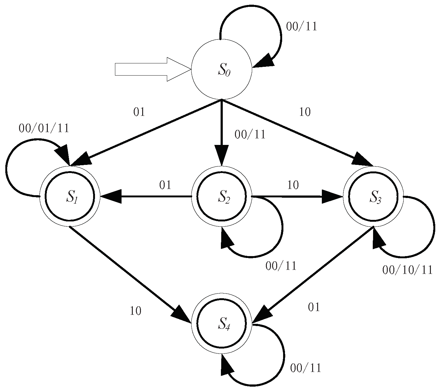
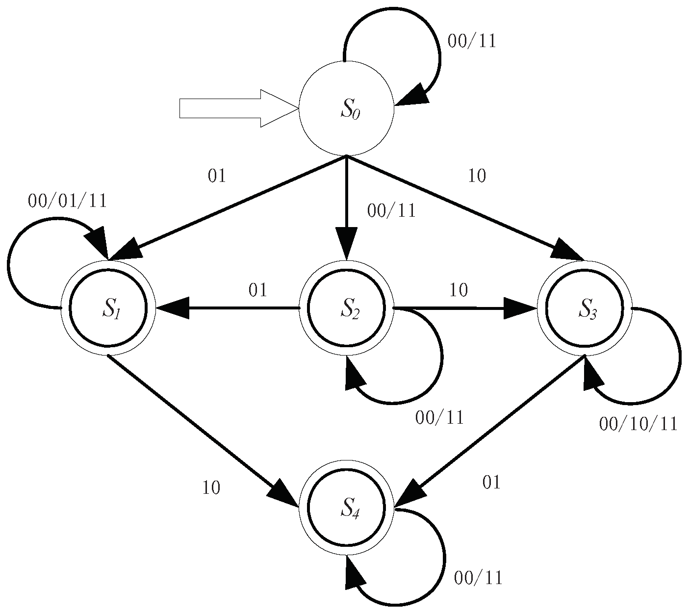
Theorem 3.

A deterministic finite automaton for row relations, denoted by $DF{A}_{row}$, is a 5-tuple $(Q,\sum ,\delta ,S_0,F)$, where $Q=\{S_0,S_1,S_2,S_3,S_4\}$ is a finite set of states, $\sum =\{e_p^0{e}_q^0{e}_p^1{e}_q^1\dots e_p^m{e}_q^m{e}_p^{m+1}{e}_q^{m+1}\dots e_p^{\left|C\right|}{e}_q^{\left|C\right|}\}(1<m<|C|,r_p,r_q\in R)$ is an input binary character string, δ is a transition function, $S_0\in Q$ is a start state, $F=\{S_1,S_2,S_3,S_4\}$ is a set of accept states. A deterministic finite automaton for row relations can be illustrated in Figure 1 as follows.

Proof. 

In a binary discernibility matrix, relations between $r_p$ and $r_q$ can be concluded as $r_q\supset r_p$, $r_p=r_q$, $r_p\supset r_q$ and $r_p\ne r_q$.

We discuss a deterministic finite automaton for row relations from four parts separately, as follows.

(1)

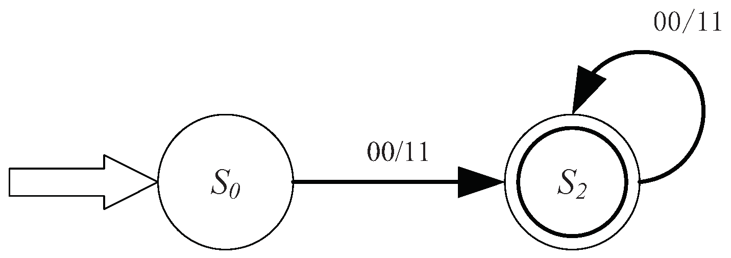
According to Definition 5 and Theorem 1, for $\forall a_m\in C$, $\forall r_p,r_q\in R$, there must be $<0,1>\in \{<e_p^m,e_q^m>:1\le p<q\le |R\left|\right\}$. Thus, the regular expression for $r_q\supset r_p$ can be defined as $[{(00/11)}^{\ast }{\left(01\right)}^{+}{(00/11)}^{\ast }{]}^{+}$. We can easily have the corresponding deterministic finite automaton in Figure 2 as:

(2)

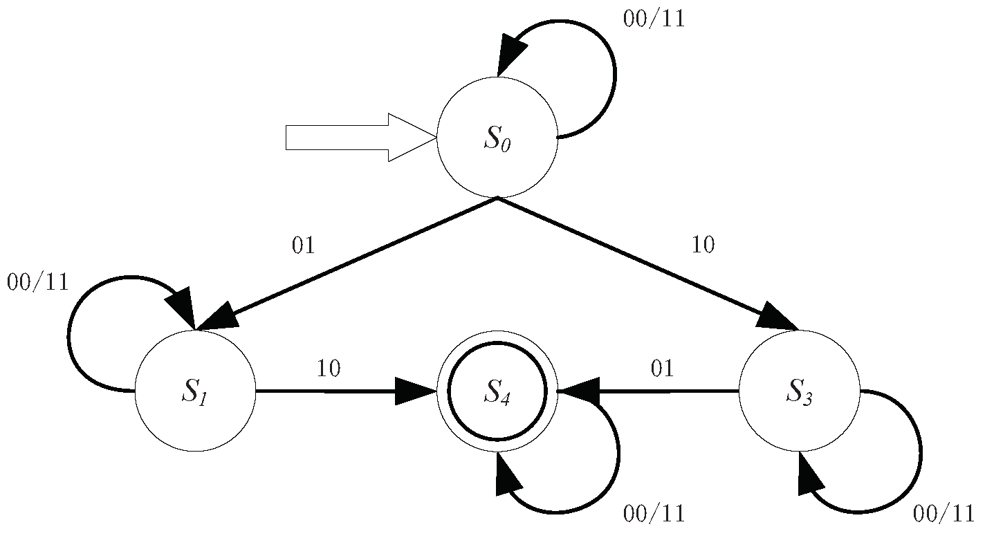
For $r_p=r_q$, there must be $<0,0>\in \{<e_p^m,e_q^m>:1\le p<q\le |R\left|\right\}$ or $<1,1>\in \{<e_p^m,e_q^m>:1\le p<q\le |R\left|\right\}$. The regular expression for $r_p=r_q$ is denoted by ${(00/11)}^{+}$. So, the corresponding deterministic finite automaton can be illustrated in Figure 3 as:

(3)

Analogous to $r_p\supset r_q$, for $r_p,r_q\in R$, there must be $<1,0>\in \{<e_p^m,e_q^m>:1\le p<q\le |R\left|\right\}$. Therefore, the regular expression for $r_p\supset r_q$ can be obtained as ${\left[{(00/11)}^{\ast }{\left(10\right)}^{+}{(00/11)}^{\ast }\right]}^{+}$. We can easily have the corresponding deterministic finite automaton in Figure 4 as:

(4)

For $r_p\ne r_q$, there must be $<1,0>\in \{<e_p^m,e_q^m>:1\le p<q\le |R\left|\right\}$ and $<0,1>\in \{<e_p^m,e_q^m>:1\le p<q\le |R\left|\right\}$. The regular expression for $r_p\ne r_q$ is denoted by ${\left[{(00/11)}^{\ast }{\left(01\right)}^{+}{(00/11)}^{\ast }{\left(10\right)}^{+}{(00/11)}^{\ast }\right]}^{+}/[{(00/11)}^{\ast }{\left(10\right)}^{+}{(00/11)}^{\ast }{\left(01\right)}^{+}{(00/11)}^{\ast }{]}^{+}$. Hence, the corresponding deterministic finite automaton can be illustrated in Figure 5 as:

One can construct a deterministic finite automaton for row relations by four deterministic finite automata shown in Figure 1.

This completes the proof. ☐

Similar to the deterministic finite automaton for row relations, we present the deterministic finite automaton for column relations in a binary discernibility matrix as follows.

Theorem 4.

A deterministic finite automaton for column relations $DF{A}_{col}$ is a 5-tuple $(Q,\sum ,\delta ,S_0,F)$, where $Q=\{S_0,S_1,S_2,S_3,S_4\}$ is a finite set of states, $\sum =\{e_0^m{e}_0^n{e}_1^m{e}_1^n\dots e_p^m{e}_p^n{e}_{p+1}^m{e}_{p+1}^n\dots e_{\left|R\right|}^m{e}_{\left|R\right|}^n\}(1<p<|R|,\forall a_m,a_n\in C)$ is an input binary character string, δ is a transition function, $S_0\in Q$ is a start state. $F=\{S_1,S_2,S_3,S_4\}$ is a set of accept states. A deterministic finite automaton for column relations can be illustrated in Figure 6 as follows:

Proof. 

This proof is similar to the proof of Theorem 3. ☐

By means of the proposed deterministic finite automata for row and column relations, we propose a quick algorithm for binary discernibility matrix simplification using deterministic finite automata (BDMSDFA) as follows:

We present the following example to explain Algorithm 3 as follows.

Algorithm 3: A quick algorithm for binary discernibility matrix simplification using deterministic finite automata, BDMSDFA.

Input: Original binary discernibility matrix $M_{BDM}$;

Output: Simplified binary discernibility matrix $M_{BDM}^{{}^{\prime }}$

1: delete the row in which all elements are 0 s; 2: compare the row relation between $r_p$ and $r_q$ by $DF{A}_{row}$ 3: for$p=1$ to $\left|R\right|$ do 4:     for $q=1$ to $\left|R\right|$ do 5:         if $r_p\supset r_q$ then 6:            delete row $r_p$ from $M_{BDM}$ 7:            break 8:         end if 9:     end for 10: end for 11: delete the column in which all elements are 0 s; 12: compare the column relation between $a_m$ and $a_n$ by $DF{A}_{col}$ 13: for$m=1$ to $\left|C\right|$ do 14:     for $n=1$ to $\left|C\right|$ do 15:         if $a_n\supset a_m$ then 16:            delete column $a_m$ from $M_{BDM}$ 17:            break. 18:         end if 19:     end for 20: end for 21: output a simplified binary discernibility matrix $M_{BDM}^{\prime }$;

Example 1.

Let $DS=(U,C\cup D,V,f)$ be a decision system shown

Table 1. A decision system.

	a1	a2	a3	a4	d
x1	1	2	0	0	1
x2	1	2	0	0	1
x3	1	2	1	1	2
x4	1	3	1	1	3
x5	2	4	1	1	4

, where the universe $U=\{x_1,x_2,x_3,x_4,x_5\}$, the condition attribute set $C=\{a_1,a_2,a_3,a_4\}$, the decision attribute set $D=\left\{d\right\}$.

For the decision system above, we have the corresponding binary discernibility matrix as follows:

$$M_{BDM}^1=\left(\begin{array}{cccc}0& 0& 0& 0\\ 0& 0& 1& 1\\ 0& 1& 1& 1\\ 1& 1& 1& 1\\ 0& 0& 1& 1\\ 0& 1& 1& 1\\ 1& 1& 1& 1\\ 0& 1& 0& 0\\ 1& 1& 0& 0\\ 1& 1& 0& 0\end{array}\right).$$

We delete the row in which all elements are 0 s in $M_{BDM}^1$, and obtain the binary discernibility matrix $M_{BDM}^2$ as follows.

$$M_{BDM}^2=\left(\begin{array}{cccc}0& 0& 1& 1\\ 0& 1& 1& 1\\ 1& 1& 1& 1\\ 0& 0& 1& 1\\ 0& 1& 1& 1\\ 1& 1& 1& 1\\ 0& 1& 0& 0\\ 1& 1& 0& 0\\ 1& 1& 0& 0\end{array}\right).$$

In the binary discernibility matrix $M_{BDM}^2$, $r_1:0011$, $r_2:0111$, $r_3:1111$, $r_4:0011$, $r_5:0111$, $r_6:1111$, $r_7:0100$, $r_8:1100$, $r_9:1100$. According to the definition of the deterministic finite automaton for row relations, we have ${\sum }_{12}=00011111$, ${\sum }_{13}=01011111$, ${\sum }_{14}=00001111$, ${\sum }_{15}=00011111$, ${\sum }_{16}=01011111$, ${\sum }_{17}=00011010$, ${\sum }_{18}=01011010$, ${\sum }_{19}=01011010$. By using the deterministic finite automaton for row relations shown in Figure 1, we can get the row relations as follows. $r_2\supset r_1$, $r_3\supset r_1$, $r_4=r_1$, $r_5\supset r_1$, $r_6\supset r_1$, $r_7\ne r_1$, $r_8\ne r_1$, $r_9\ne r_1$. Therefore, we delete $r_2$, $r_3$, $r_5$ and $r_6$. Similarly, we get $r_8\supset r_7$ and $r_9\supset r_7$, $r_4\ne r_7$, and then delete $r_8$ and $r_9$. Therefore, we have the following binary discernibility matrix:

$$M_{BDM}^3=\left(\begin{array}{cccc}0& 0& 1& 1\\ 0& 0& 1& 1\\ 0& 1& 0& 0\end{array}\right).$$

We delete the column in which all elements are 0 s in $M_{BDM}^3$, and have

$$M_{BDM}^4=\left(\begin{array}{ccc}0& 1& 1\\ 0& 1& 1\\ 1& 0& 0\end{array}\right).$$

In the binary discernibility matrix $M_{BDM}^4$, $a_1:001$, $a_2:110$, $a_3:110$. According to the definition of deterministic finite automaton for column relations, we have ${\sum }_{12}=010110$, ${\sum }_{13}=010110$, ${\sum }_{23}=111100$. By using the deterministic finite automaton for column relations shown in Figure 6, we have $a_1\ne a_2$, $a_1\ne a_3$, $a_2=a_3$. Thus, we cannot delete any column in $M_{BDM}^4$, and get the following binary discernibility matrix.

$$M_{BDM}^5=\left(\begin{array}{ccc}0& 1& 1\\ 0& 1& 1\\ 1& 0& 0\end{array}\right).$$

A $10\times 4$ matrix $M_{BDM}^1$ is compressed to a $3\times 3$ matrix $M_{BDM}^5$. The simplified binary discernibility matrix with fewer objects or columns will be help in improving the efficiency of attribute reduction.

Assume that $t=\left|R\right|$ and $s=\left|C\right|$, the upper bound of time complexity of BDMR is $3ts(t+s-2)$, the lower bound of time complexity of BDMR is $2ts(t+s-2)$. The upper bound of time complexity of IBDMR is $3ts(t+s-2)$ and the lower bound of the worst-case time complexity of IBDMR is $2ts(t+s-2)$. By employing deterministic finite automata, the algorithm complexity of BDMSDFA is $ts(t+s-2)$. Obviously, the time complexity of BDMSDFA is lower than that of BDMR and IBDMR. Therefore, it is concluded that the proposed algorithm BDMSDFA reduces the computational time for binary discernibility matrix simplification in general.

The advantages of the proposed method are expressed as follows. (1) Deterministic finite automata in a binary discernibility matrix are constructed, it can provide an understandable approach to comparing the relationships of different rows (columns) quickly. (2) Based on deterministic finite automata, a high efficiency algorithm of binary discernibility matrix simplification is developed. Theoretical analyses and experimental results indicate that the proposed algorithm is effective and efficient. It should be noted that the proposed method is based on Pawlak decision systems, but not suitable for generalized decision systems, such as incomplete decision systems, interval-valued decision systems and fuzzy decision systems. Deterministic finite automata in generalized decision systems will be investigated in the future.

5. Experimental Results and Analyses

The objective of the following experiments in this section is to demonstrate the high efficiency of the algorithm BDMSDFA. The experiments are divided into two aspects. In one aspect, we employ 10 datasets in

Table 2. Time consumption of BDMR, IBDMR and BDMSDFA.

Data Sets	Num. of Objects	Num. of Attributes	Num. of Rows	Num. of Columns	Time of BDMR (ms)	Time of IBDMR (ms)	Time of BDMSDFA (ms)
Labor_neg	40	15	52	14	2	2	1
Lung-cancer	32	57	206	53	11	9	3
Heart_statlog	270	14	96	13	32	27	14
Autos	250	26	36	19	75	68	36
Credit_a	690	16	27	12	113	105	55
Breast_w	699	10	20	9	75	73	29
Anneal	898	39	9	9	206	194	134
Promoters	106	58	2761	57	1517	936	398
Dermatology	366	35	1347	31	3239	2638	1318
Connect_4	67,557	43	697	42	2,444,328	2,433,863	1,759,917

to verify the performance of time consumption of BDMR, IBDMR and BDMSDFA. In the other aspect, the computational times of algorithms BDMR, IBDMR and BDMSDFA with the increase of the size of attributes (or objects) are calculated respectively. We carry out three algorithms on a personal computer with Windows 8.1 (64 bit) and Inter(R) Core(TM) i5-4200U, 1.6 GHz and 4 GB memory. The software is Microsoft Visual Studio 2017 version 15.9 and C++. Data sets used in the experiments are all downloaded from UCI repository of machine learning data sets (http://archive.ics.uci.edu/ml/datasets.html).

Table 2 indicates the computational time of BDMR, IBDMR and BDMSDFA on the 10 data sets. We can see that the algorithm BDMSDFA is much faster than the algorithms BDMR and IBDMR. The computational times of three algorithms follows this order: BDMR ≥ IBDMR > BDMSDFA. The computational time of BDMSDFA is the minimum among the three algorithms. For the data set Auto in Table 2, the computational times of BDMR and IBDMR are 75 ms and 68 ms, while that of BDMSDFA is 36 ms. For the data set Credit_a, the computational times of BDMR and IBDMR are 113 ms and 105 ms, while that of BDMSDFA is 55 ms. For some data sets in Table 2, the computational time of BDMSDFA can reduce over half the computational time of BDMR or IBDMR. In Table 2, for the data set Breast_w, the computational times of BDMR and IBDMR are 75 ms and 73 ms, while that of BDMSDFA is 29 ms. For the data set Promoters, the computational times of BDMR and IBDMR are 1517 ms and 936 ms, while that of BDMSDFA is only 398 ms. For the date sets such as Lung-cancer, Credit_a, Breast_w, Anneal, the computational time of BDMR is close to that of IBDMR. For the data set Labor_neg, the computational time of BDMR is equivalent to that of IBDMR. For each data set in Table 2, difference between BDMR and IBDMR is relatively smaller than difference between BDMR (IBDMR) and BDMSDFA.

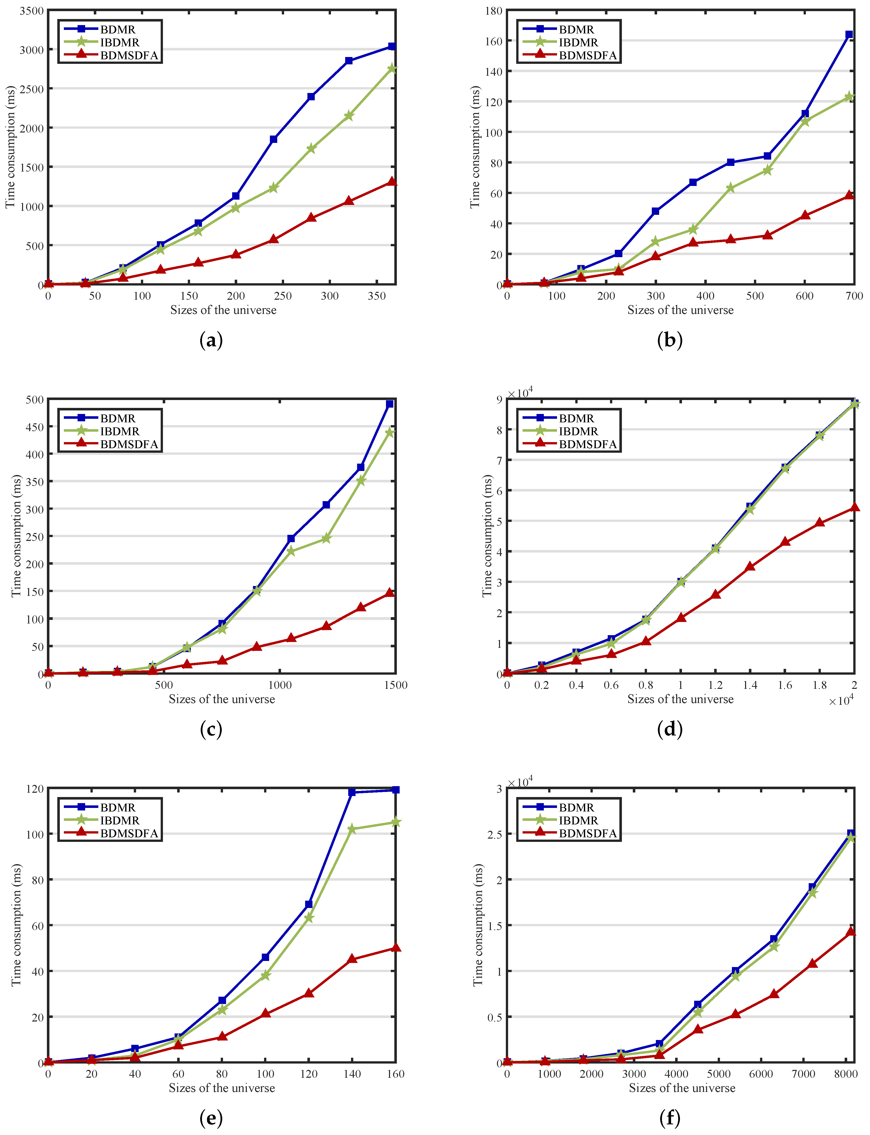
We compare the computational times of BDMR, IBDMR and BDMSDFA with the increase of the size of objects. In Figure 7a–f, the x-coordinate pertains to the size of objects in the universe, while the y-coordinate concerns the time consumption of algorithms. We employ 6 data sets (Dermatlogy, Credit_a, Controceptive_Method_Choice, Letter, Flag and Mushroom) to verify the performance of time consumption of BDMR, IBDMR and BDMSDFA. When dealing with the same UCI data sets, the computational time of BDMSDFA is less than that of BDMR and IBDMR, in other words, BDMSDFA is more efficient than BDMR and IBDMR. Figure 7 shows more detailed change trends of each algorithm with the number of objects increasing. The computational times of three algorithms increase with the increase of the number of objects simultaneously. It is obvious to see that the slope of the curve of BDMSDFA is smaller than the curve of BDMR or IBDMR, and the computational time of BDMSDFA increases slowly. The differences between BDMR (IBDMR) and BDMSDFA become distinctly larger when the size of the objects increases. In Figure 7c, the difference of BDMR (IBDMR) and BDMSDFA is not obviously different at the beginning. The computational time of DBMR (IBDMR) increases distinctly when the number of objects is over 450. The computational time of algorithm BDMR increases by 479 ms when the number of objects rises from 450 to 1473, whereas the computational time of algorithm BDMSDFA increases by only 141 ms. In Figure 7e, the computational time of the algorithm IBDMR increases by 104 ms when the number of objects rises from 20 to 160, whereas the time consumption of algorithm BDMSDFA increases by only 49.

In Figure 8a–f, the x-coordinate pertains to the size of attributes, while the y-coordinate concerns the time consumption of algorithms. We also take 6 data sets (Dermatlogy, Credit_a, Controceptive_Method_Choice, Letter, Flag and Mushroom) to verify the performance of the computational times of BDMR, IBDMR and BDMSDFA. The curve of BDMR is similar to that of IBDMR. The curve of BDMSDFA is under the curves of BDMR and IBDMR. Then, the computational time of BDMSDFA is less than that of BDMR or IBDMR. In Figure 8b, the computational time of algorithms BDMR and IBDMR increase by 164 ms and 123 ms respectively, while the computational time of algorithm BDMSDFA increases by 58 ms. In Figure 8c, the curves of BDMR and IBDMR raise profoundly when the size of the attributes increases. In Figure 8e, the computational time of algorithm IBDMR increases from 4 ms to 105 ms when the number of objects rises from 3 to 24, while the computational time of algorithm BDMSDFA increasedly from 2 ms to 50 ms. For Figure 8a–f, it is concluded that the efficiency of BDMSDFA is higher than that of BDMR or IBDMR with the increase of the number of attributes. Difference between BDMR and IBDMR is relatively smaller than difference between BDMR (IBDMR) and BDMSDFA. The computational times of three algorithms increase with the increase of the number of attributes monotonously. When dealing with the same situation, the computational time of BDMSDFA is the minimum among the three algorithms.

Experimental analyses and results show a high efficiency of the algorithm BDMSDFA. The proposed simplification algorithm using deterministic finite automata can be applied as a preprocessing technique for data compression and attribute reduction in large-scale data sets.

6. Conclusions

Original binary discernibility matrices which are not simplified usually have irrelative objects and attributes. These irrelative objects and attributes may lead to inefficiency in attribute reduction, knowledge acquisition, etc. To tackle this problem, a quick method of comparing the relationships of different rows (columns) are introduced in binary discernibility matrices. By using deterministic finite automata, a quick algorithm for binary discernibility matrix simplification (BDMSDFA) is developed. The experiment results indicate that DBMSDFA can get higher performance in the efficiency of binary discernibility matrix simplification. The contributions of this paper can be summarized as follows.

(1)

We define row (or column) relations which are used for constructing deterministic finite automata.

(2)

Deterministic finite automata are firstly used for comparing the relationships of different rows (columns) in a binary discernibility matrix.

(3)

Based on deterministic finite automata, a quick algorithm for binary discernibility matrix simplification is developed. Experimental results indicate that the relationship between the time consumption of BDMSDFA and the number of objects (attributes) is strictly monotonic. With the increase of the size of objects (attributes), the algorithm BDMSDFA is more efficient than BDMR and IBDMR.

It is noted that the proposed quick simplification algorithm for discernibility matrix is only suitable for completed decision systems. However, in practical applications, there exists many generalized decision systems, such as incomplete decision systems, interval-valued decision systems, etc. Researches on quick simplification algorithms in generalized decision systems will be investigated. Combing the researches on fuzzy sets [33,34,35,36], we will propose the fuzzy binary discernibility matrix. Some applications of the (fuzzy) binary discernibility matrix simplification will also be studied in the future.