Tri-SIFT: A Triangulation-Based Detection and Matching Algorithm for Fish-Eye Images

Abstract
1. Introduction
2. Related Work
3. SIFT Algorithm Theory
4. Tri-SIFT Algorithm
4.1. Back-Projection
4.2. Triangulation
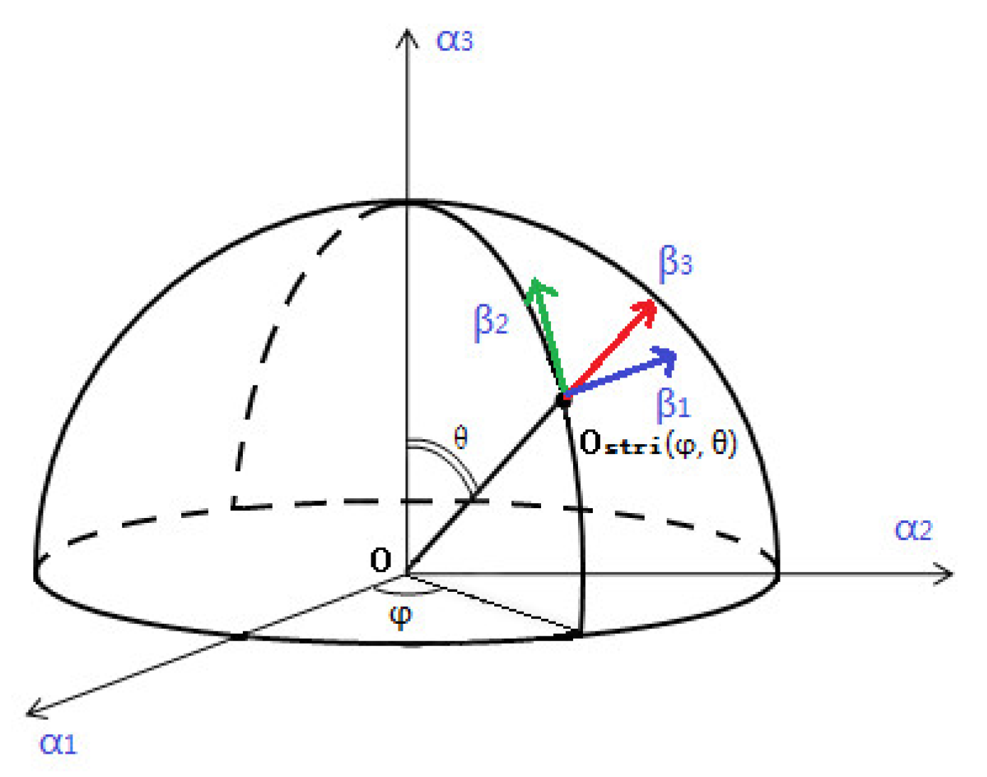
4.3. Orientation
| Algorithm 1 Algorithm for the computation of the dominant orientation |
|
4.4. The Descriptor Construction
| Algorithm 2 Algorithm for the computation of LSD |
|
5. Experiment
6. Conclusions
Author Contributions
Funding
Conflicts of Interest
References
- Barreto, J.; Santos, J.M.; Menezes, P.; Fonseca, F. Ray-based calibration of rigid medical endoscopes. Available online: https://www.researchgate.net/publication/29622069_Raybased_Calibration_of_Rigid_Medical_Endoscopes (accessed on 23 November 2018).
- Baker, P.; Fermuller, C.; Aloimonos, Y.; Pless, R. A spherical eye from multiple cameras (makes better models of the world). In Proceedings of the 2001 IEEE Computer Society Conference on Computer Vision and Pattern Recognition, Kauai, HI, USA, 8–14 December 2001. [Google Scholar]
- Liu, N.; Zhang, B.; Jiao, Y.; Zhu, J. Feature matching method for uncorrected fisheye lens image. In Seventh International Symposium on Precision Mechanical Measurements; SPIE Press: Bellingham, WA, USA, 2016. [Google Scholar]
- Kim, D.; Paik, J. Three-dimensional simulation method of fish-eye lens distortion for a vehicle backup rear-view camera. JOSA A 2015, 32, 1337–1343. [Google Scholar] [CrossRef] [PubMed]
- Zhang, B.; Jia, Y.; Röning, J.; Feng, W. Feature matching method study for uncorrected fish-eye lens image. In Intelligent Robots and Computer Vision XXXII: Algorithms and Techniques; SPIE Press: Bellingham, WA, USA, 2015. [Google Scholar]
- Hansen, P.I.; Corke, P.; Boles, W.; Daniilidis, K. Scale-invariant features on the sphere. In Proceedings of the IEEE 11th International Conference on Computer Vision, Rio de Janeiro, Brazil, 14–20 October 2007. [Google Scholar]
- Hansen, P.; Corke, P.; Boles, W. Wide-angle visual feature matching for outdoor localization. Int. J. Robotics Res. 2010, 29, 267–297. [Google Scholar] [CrossRef]
- Miyamoto, K. Fish eye lens. JOSA 1964, 54, 1060–1061. [Google Scholar] [CrossRef]
- Lowe, D.G. Object recognition from local scale-invariant features. In Proceedings of the International Conference on Computer Vision, Kerkyra, Greece, 20–27 September 1999; pp. 1150–1157. [Google Scholar]
- Lourenço, M.; Barreto, J.P.; Vasconcelos, F. Srd-sift: Keypoint detection and matching in images with radial distortion. T-RO 2012, 28, 752–760. [Google Scholar] [CrossRef]
- Hughes, C.; Denny, P.; Glavin, M.; Jones, E. Equidistant fish-eye calibration and rectification by vanishing point extraction. TPAMI 2010, 32, 2289–2296. [Google Scholar] [CrossRef] [PubMed]
- Se, S.; Lowe, D.; Little, J. Mobile robot localization and mapping with uncertainty using scale-invariant visual landmarks. Int. J. Robotics Res. 2002, 21, 735–758. [Google Scholar] [CrossRef]
- Bay, H.; Ess, A.; Tuytelaars, T.; Van Gool, L. Speeded-up robust features (SURF). Comput. Vis. Image Und. 2008, 110, 346–359. [Google Scholar] [CrossRef]
- Wan, L.; Li, X.; Feng, W.; Long, B.; Zhu, J. Matching method of fish-eye image based on CS-LBP and MSCR regions. Available online: http://cea.ceaj.org/EN/column/column105.shtml (accessed on 22 November 2018).
- DING, C.X.; JIAO, Y.K.; LIU, L. Stereo Matching Method of Fisheye Lens Image Based on MSER and ASIFT. Available online: http://en.cnki.com.cn/Article_en/CJFDTOTAL-HGZD201801008.htm (accessed on 22 November 2018).
- Kannala, J.; Brandt, S.S. A generic camera model and calibration method for conventional, wide-angle, and fish-eye lenses. TPAMI 2006, 28, 1335–1340. [Google Scholar] [CrossRef] [PubMed]
- Arfaoui, A.; Thibault, S. Fisheye lens calibration using virtual grid. Appl. Opt. 2013, 52, 2577–2583. [Google Scholar] [CrossRef] [PubMed]
- Kanatani, K. Calibration of Ultrawide Fisheye Lens Cameras by Eigenvalue Minimization. TPAMI 2013, 35, 813–822. [Google Scholar] [CrossRef] [PubMed]
- Mikolajczyk, K.; Schmid, C. A performance evaluation of local descriptors. TPAMI 2005, 27, 1615–1630. [Google Scholar] [CrossRef] [PubMed]


| SIFT | Rect-SIFT | RD-SIFT | Tri-SIFT | |||||
|---|---|---|---|---|---|---|---|---|
| Initial Match | Correct Match | Initial Match | Correct Match | Initial Match | Correct Match | Initial Match | Correct Match | |
| Scale | 170 | 153 | 238 | 198 | 251 | 209 | 243 | 216 |
| Translation | 97 | 83 | 102 | 91 | 116 | 89 | 108 | 98 |
| Affine | 114 | 102 | 128 | 106 | 151 | 119 | 136 | 125 |
© 2018 by the authors. Licensee MDPI, Basel, Switzerland. This article is an open access article distributed under the terms and conditions of the Creative Commons Attribution (CC BY) license (http://creativecommons.org/licenses/by/4.0/).
Share and Cite
Wang, E.; Jiao, J.; Yang, J.; Liang, D.; Tian, J. Tri-SIFT: A Triangulation-Based Detection and Matching Algorithm for Fish-Eye Images. Information 2018, 9, 299. https://doi.org/10.3390/info9120299
Wang E, Jiao J, Yang J, Liang D, Tian J. Tri-SIFT: A Triangulation-Based Detection and Matching Algorithm for Fish-Eye Images. Information. 2018; 9(12):299. https://doi.org/10.3390/info9120299
Chicago/Turabian StyleWang, Ende, Jinlei Jiao, Jingchao Yang, Dongyi Liang, and Jiandong Tian. 2018. "Tri-SIFT: A Triangulation-Based Detection and Matching Algorithm for Fish-Eye Images" Information 9, no. 12: 299. https://doi.org/10.3390/info9120299
APA StyleWang, E., Jiao, J., Yang, J., Liang, D., & Tian, J. (2018). Tri-SIFT: A Triangulation-Based Detection and Matching Algorithm for Fish-Eye Images. Information, 9(12), 299. https://doi.org/10.3390/info9120299