Hybrid Metaheuristics to the Automatic Selection of Features and Members of Classifier Ensembles

Abstract

Metaheuristic algorithms have been applied to a wide range of global optimization problems. Basically, these techniques can be applied to problems in which a good solution must be found, providing imperfect or incomplete knowledge about the optimal solution. However, the concept of combining metaheuristics in an efficient way has emerged recently, in a field called hybridization of metaheuristics or, simply, hybrid metaheuristics. As a result of this, hybrid metaheuristics can be successfully applied in different optimization problems. In this paper, two hybrid metaheuristics, MAMH (Multiagent Metaheuristic Hybridization) and MAGMA (Multiagent Metaheuristic Architecture), are adapted to be applied in the automatic design of ensemble systems, in both mono- and multi-objective versions. To validate the feasibility of these hybrid techniques, we conducted an empirical investigation, performing a comparative analysis between them and traditional metaheuristics as well as existing existing ensemble generation methods. Our findings demonstrate a competitive performance of both techniques, in which a hybrid technique provided the lowest error rate for most of the analyzed objective functions.

1. Introduction

Classification algorithms assign labels to objects (instances or examples) based on a predefined set of labels. Several classification models have been proposed in the literature [1]. However, there is no algorithm that achieves good performance for all domain problems. Therefore, the idea of combining different algorithms in one classification structure has emerged. These structures, called ensemble systems, are composed of a set of classification algorithms (base classifiers), organized in a parallel way (all classifiers are applied to the same task), and a combination method with the aim of increasing the classification accuracy of a classification system. In other words, instead of using only one classification algorithm, an ensemble uses a set of classifiers whose outputs are combined to provide a final output, which is expected to be more precise than those generated individually by the classification algorithms [2]. A good review of ensemble of classifiers can be found in [3,4,5].

An important issue in the design of ensemble systems is the parameter setting. More specifically, the selection of the base classifiers, features and the combination method plays an important role in the design of effective ensemble systems. Although feature selection may not be a parameter of the ensemble system structure, feature selection may have a strong effect in the performance of these systems and, therefore, it will be considered as a pre-processing parameter. The parameter setting of an ensemble system can be modeled as an optimization problem, in which the parameter set that provides the best ensemble system must be found. When considering the ensemble parameter selection as an optimization problem, it is possible to apply search strategies to solve these problems, applying exhaustive or metaheuristic approaches. Among the metaheuristic search algorithms, the most popular techniques are the population-based ones (genetic algorithm, particle swarm intelligence, ant colony optimization, et.c) since they have been successfully applied in traditional classification algorithms as well as ensemble systems [6].

The idea of efficiently combining metaheuristics has emerged lately, in a field called hybridization of metaheuristics or hybrid metaheuristics. The main motivation for hybridization is to combine the advantages of each algorithm to form a hybrid algorithm, trying to minimize any substantial disadvantage of the combined algorithms. Some hybridization techniques have been proposed in the literature (e.g., [7,8,9,10,11]). These hybrid metaheuristics have been successfully applied to traditional optimization problems. In [7], for instance, the mono-objective MAMH (Multiagent Architecture for Metaheuristic Hybridization) architecture is proposed. The idea is to present a PSO-based multiagent system, using a multiagent framework with some swarm intelligence elements. According to the authors, MAMH can be considered as a simple hybrid architecture, taking advantage of the full potential of several metaheuristics and using theses advantages to better perform a given optimization problem. Another promising hybrid architecture is mono-objective MAGMA (Multiagent Metaheuristic Architecture), which was originally proposed by Milano et al. [12]. This architecture has also been efficiently applied to traditional optimization problems [12].

To the best of the authors knowledge, there is no study using hybrid architecture in the optimization of ensemble systems. Therefore, we aimed to adapt two promising hybrid architectures, MAMH and MAGMA, to be applied in the automatic design of classifier ensembles (or ensemble systems), which is a well-known optimization problem of the Pattern Recognition field. Specifically, the use of MAMH and MAGMA architectures to define two important parameters of classifier ensembles (the individual classifiers and features) was investigated. In this investigation, two important aspects of an ensemble system were considered, accuracy and diversity, using them as objective function in both mono- and multi-objective versions of the analyzed architectures. For accuracy, the error rate was used as objective function, while, for diversity, two diversity measures were used as objective functions, good and bad diversity [13].

To investigate the potential of the hybrid architectures as an ensemble generator method, an empirical investigation was conducted in which the hybrid metaheuristics were evaluated using 26 classification datasets, in both mono- and multi-objective contexts. A comparative analysis was also performed, comparing the performance of the hybrid architectures to some traditional metaheuristics as well as to traditional and recent ensemble generation techniques.

In [14], our first attempt to use one hybrid architecture (MAMH) for the automatic design of ensemble systems (features and base classifiers), when optimizing the classification error and good and bad diversity, is presented. However, in [14], we only analyzed these three objectives separately, in the mono-objective context. In this paper, we extend the work done in [14], using one more hybrid architecture and performing a comparative analysis with traditional population and trajectory-based metaheuristics. In addition, an empirical analysis with all different combinations of error rate, good diversity and bad diversity as optimization objectives is presented. In doing this investigation, we aimed at defining the set of objectives that generates the most accurate ensembles. In addition, our aim was to analyze whether the diversity measures can have an important role in the design of effective and robust classifier ensembles. Hence, we can describe the main contributions of this papers as follows:

• Propose the multi-objective MAMH: In [7], only the mono-objective version is proposed. In this paper, we extend the work in [7] by presenting its multi-objective version.
• Propose the multi-objective MAGMA: In [12], the mono-objective MAGMA is proposed. In this paper, we extend the work in [12] by presenting its multi-objective version.
• We adapt these two metaheuristics to the automatic design of ensemble of classifiers.
• We compare the results delivered by both hybrid metaheuristics when accuracy, good diversity and bad diversity were used as objectives to generate robust classifier ensembles.

This paper is divided into six sections and is organized as follows. Section 2 describes the research related to the subject of this paper, while the proposed hybrid architectures are described in Section 3. Section 4 presents the methodology employed in the experimental work of this paper, while an analysis of the results provided by the empirical analysis is shown in Section 5. Finally, Section 6 presents the final remarks of this paper.

2. State-of-the-Art: Optimization Techniques for Classifier Ensembles

The definition of the best technique for a particular classification application is a challenging problem and has been addressed by several authors [15,16,17,18,19,20,21]. This problem has been treated as a meta-learning problem [17,22], automatic selection of machine learning (auto-ML) [16,18,20] or an optimization problem [15,19,21]. In [18], for instance, the authors used an auto-ML technique to define the best classification algorithm, along with the best set of parameters, for a specific classification problem. Usually, these classification algorithms can be either single classifiers or ensemble systems. In this study, the main focus was ensemble systems, more specifically the selection of features, which is not fully exploited in auto-ML techniques, as well as members of an ensemble. Therefore, it was treated as an optimization problem.

Despite the high number of studies, finding an optimal parameter set that maximizes classification accuracy of an ensemble system is still an open problem. The search space for all parameters of an ensemble system (classifier type, size, classifier parameters, combination method and feature selection) is very large. For simplicity, we considered two important parameters: members and feature selection.

When using optimization techniques in the design of ensemble systems, there are several studies involving the use of these techniques in the definition of the best feature set [23,24,25,26] and the members of an ensemble [27,28,29]. In the selection of the feature set, different optimization techniques have been applied, most of them population-based techniques, individually. Examples of these techniques are bee colony optimization [24], particle swarm optimization (PSO) [30] and genetic algorithms [26]. On the contrary, some studies have combined different optimization techniques, for example, in [23],  bee colony optimization is combined with particle swarm optimization for feature selection and genetic algorithms for the configuration of some ensemble parameters. Additionally, in [25], different metaheuristics are applied to the selection of feature set in ensembles.

In the selection of ensemble members, in [29], the authors proposed the use of genetic algorithms to select the set of weak classifiers and their associated weights. The genetic algorithm applied a new penalized fitness function that aimed to limit the number of weak classifiers and control the effects of outliers. According to the authors, the proposed method proved to be more resistant to outliers and resulted in achieving simpler predictive models than AdaBoost and GentleBoost.

As can be observed, the majority of studies of optimization techniques for the automatic design of ensemble system apply only mono-objective techniques. Nevertheless, some effort has been done to employ multi-objective techniques in the context of ensembles [31,32,33,34]. In [32], for instance, the authors proposed the use of an optimization technique to design ensemble systems, taking into account the accuracy and diversity. However, different from this paper, it does not address diversity as an optimization objective. Another study that uses an optimization technique, simulated annealing, to calculate competence and diversity of ensemble components is [31]. However, once again, it uses diversity measures as a guide to select members or features in ensemble systems, not in the multi-objective context. In [33], the authors proposed a framework to obtain ensembles of classifiers from a Multi-objective Evolutionary Algorithm (MOEA), applying two objectives, the Correct Classification Rate or Accuracy (CCR) and the Minimum Sensitivity (MS) of all classes. However, different from this paper, the MOE algorithm was applied to select the classifiers of an ensemble individually, not considering the combination of these classifiers as a whole.

In either the mono- or multi-objective context, to the best of the authors knowledge, there is no study using hybrid metaheuristics in the optimization of ensemble systems. In [15], for instance, an exploratory study with several optimization techniques in the design of ensemble systems is presented. In the presented study, the authors investigated several techniques in both mono- and multi-objective versions. As a result of this study, the authors stated that the choice of the optimization technique is an objective-dependent selection and no single technique is the best selection for all cases (mono- and multi-objective as well as datasets). The results obtained in [15] are the main motivation for the investigation performed here.

3. Hybrid Metaheuristics

As mentioned previously, metaheuristic algorithms have been extensively used to solve global optimization problems and examples of metaheuristic applications can be found in [35,36,37,38]. Recently, the concept of efficiently combining metaheuristics has emerged, in a field called hybridization of metaheuristics or, simply, hybrid metaheuristics. The main aim of hybrid metaheuristics is to exploit the complementary particularities provided by different optimization strategies [39]. Undeniably, the selection of an adequate combination of complementary algorithmic concepts can play an important role in achieving high performance when solving several difficult optimization problems. These hybrid systems have been successfully applied in traditional optimization problems. There are some hybridizations proposed in the literature (e.g., [7,8,9,10,11]). In the next two subsections, two hybrid architectures, MAMH and MAGMA are described.

3.1. MAMH Architecture

The MAMH (Multi-agent Metaheuristic Hybridization) algorithm used in this paper is an extension of the mono-objective MAMH architecture first presented in [7]. The original MAMH was proposed to be a PSO-based multi-agent platform for the hybridization of metaheuristics and was originally proposed to solve mono-objective optimization problems. To adapt the PSO algorithm for MAMH, all PSO components, such as particles, positions, velocities, operations that modify the positions and neighbourhoods, must be adapted. Hence, each particle in MAHM can be considered as an autonomous agent with its own memory, decision and learning methods. Additionally, the environment used in a multi-agent system is represented by the optimization search space of the analyzed problem. The agent’s perceptions are represented by the positions and strategies of other agents. Finally, all agents need to find the best possible solution.In relation to the decision strategies, they are represented by the metaheuristics that can cause any changes in the agent’s position (location in the search space). The learning strategies of the PSO-based agent will be used in the decision-making process, defining the decisions (metaheuristic) that will be applied as well as which kind of information will be shared with other agents. Finally, the agent’s actions are represented by movements in the search space as a result of a decision-making strategy that updates the value of the objective function.

Algorithm 1 illustrates the adapted version of the MAMH algorithm, which is applied in the automatic design of classifier ensembles. As can be observed, this algorithm has three parameters as input: the number of agents/particles (size), the pool of decision strategies (ED) and the pool of learning strategies (EA).

Algorithm 1 MAMH.

Require:$size,ED,EA$

1: $g_{bes{t}_i}$ ← ∞

2: for i ≤ 1 size do

3: $x_i\leftarrow$ make_position($p_i$)

4: $p_{bes{t}_i}\leftarrow inf$

5: select_decision_strategy($p_i,ED$)

6: select_learning_strategy($p_i,EA$)

7: end for

8: while not Stop-Condition do

9: for i ≤ 1 size do

10: if$fitness\left(x_i\right)<fitness(p_{bes{t}_i}$) then

11: $p_{bes{t}_i}\leftarrow x_i$

12: end if

13: if $fitness\left(x_i\right)<fitness\left(g_{bes{t}_i}\right)$ then

14: $g_{bes{t}_i}\leftarrow x_i$

15: end if

16: end for

17: for i ≤ 1 size do

18: start learning method($p_i$)

19: $x_i$ apply decision method($p_i$)

20: $x_{best}\leftarrow$ random($p_{bes{t}_i},g_{bes{t}_i}$)

21: execute velocity operator($x_i,x_{dest}$)

22: end for

23: end while

24: return $g_{bes{t}_i}$

As a PSO-based procedure, for a given agent (particle) $p_i$, $x_i$ represents its current position, $p_{bes{t}_i}$ represents the local best position and $g_{bes{t}_i}$ represents the global best position. This algorithm is based on the management of the learning and decision strategies of the agents. The decision strategies change the position of the particles by applying the most suitable metaheuristic in its current position. Conversely, the learning strategies control which decision strategies are active.

The MAMH can apply different decision strategies simultaneously. In this study, we chose to use GRASP and Genetic algorithms as decision strategies. Additionally, the learning strategy was set to allow up to three failures ($T=3$) of a decision strategy. Finally, the MAMH algorithm is composed of a set of agents and each one provides a solution, $x_i$ for the analyzed problem. This solution consists of the agent’s position in the search space. In addition, each agent has three distinct behaviors:

• The first behavior is to explore the search space that consists of applying the selected learning strategy. It consists of applying a traditional metaheuristic to modify its position in the search space. When a learning strategy is changed, each metaheuristic uses the current position of agent $x_i$ to determine the starting point in the search space.
• The second action consists of returning to the best position found by an agent until the current state, $p_{bes{t}_i}$. This is also done using the path re-linking speed operator, starting from $x_i$ towards $p_{bes{t}_i}$. In doing this, the decision strategy is also modified to match the decision strategy used to generate $p_{bes{t}_i}$. This will also reset the fault counter to zero.
• In the third behavior, the agent will try to move to the position of the best agent $g_{bes{t}_i}$. Once again, this is done using the path re-linking speed operator, starting from $x_i$ towards $g_{bes{t}_i}$. In doing this, the decision strategy is also modified to match the decision strategy used to generate $g_{bes{t}_i}$. This will also reset the fault counter to zero.

The selection of the current behavior is based on a probabilistic choice (random function in line 20), with a different selection rate for each behavior. After an initial analysis, in this study, we used $F_b=85\%$, $S_b=10\%$ and $T_b=5\%$ rates for the first, second and third behaviors, respectively.

The Multi-Objective MAMH

For the multi-objective MAMH version, each agent contains the following information: (1) a set of non-dominated solutions $ND$; (2) its current learning strategy or metaheuristic, m; (3) the local best set of non-dominated solutions $N{D}^{\prime }$ (based on a multi-objective metric); and (4) the metaheuristic that provided the best set of non-dominated solutions, $m^{\prime }$. Each agent has three possible states:

• Intensification: The application of the current metaheuristic m, modifying the position of the particle.

  (a)

  The metaheuristic input is the set of non-dominated solutions of the previous step. For the population-based techniques, if the set of non-dominated solutions is lower than the size of the population, the remaining individuals are randomly chosen. For the trajectory-based techniques in which only one solution is used, a solution is randomly chosen from the set of non-dominated solutions.

  (b)

  After the application of the metaheuristic m, the new set of non-dominated solutions is created. If its current set of non-dominated solutions $ND$ is better than its local best $N{D}^{\prime }$ (based on a multi-objective metric), $ND$ replaces $N{D}^{\prime }$.

  (c)

  In the case a metaheuristic fails to provide a better set of non-dominated solutions for T times, it will be replaced by a more promising metaheuristic. A possible metaheuristic is the one used by one of the agent’s neighbour which has a better performance (based on a multi-objective metric). Among the possible neighbours, this selection becomes a random one.

• The particle follows its best position (local best). In this case, the current set of non-dominated solutions $ND$ is merged with its local best, $N{D}^{\prime }$, removing the dominated solutions and selecting the best solutions (based on a multi-objective metric). The current metaheuristic is now the one that belongs to the local best.
• The particle follows the best overall position (global best). In this case, the current set of non-dominated solutions $ND$ is merged with the global best, $N{D}_g^{\prime }$, removing the dominated solutions and selecting the best solutions (based on a multi-objective metric). The current metaheuristics is now the one that belongs to the global best.

The choice of the state is made in a random way, respecting a probability distribution. As we wanted to assess the hybridization of the metaheuristics, we selected a high probability for the intensification state, 70%. In addition, we selected 20% for the second state and 10% for the third one. These values are selected since we would a higher change of the particle to follow its own steps than the neighbours ones. Finally, these states are performed until a stopping condition is met.

The multi-objective metric used in this paper is hyper-volume, described in Section 4.3.2.

3.2. MAGMA Architecture

MAGMA architecture (Multi-agent metaheuristic Architecture) proposed by Milano et al. [12] is an architecture organized in four layers. Figure 1 presents the general MAGMA architecture, adapted from [12]. In this architecture, each layer can be represented by one or more agents. The first layer (Layer 0) builds viable solutions to the next layer. The second layer (Layer 1) applies refinement heuristics on the provided solutions. The third layer (Layer 2) includes employed agents with a global vision of space. In other words, agents have to provide mechanisms to guide solutions for search space regions, providing an escape mechanism for the local minimum. The fourth layer (Layer 3) coordinates different search strategies involving communication and synchronization among agents.

The MAGMA architecture was originally proposed to apply up to six specializations for mono-objective optimization problems [12]. In other words, according to the original proposal, up to six different metaheuristics could be implemented, following the foundations defined in this architecture. However, in the empirical analysis of the original proposal, the cooperative search was composed of GRASP and Memetic algorithms. For the GRASP algorithm, Layer 0 has a random and greedy algorithm; Layer 1 has a local search (minimization of objective functions); and Layer 2 stores the best solutions. For the Memetic algorithm, the solutions are randomly generated in Layer 0; Layer 1 has a local search; and Layer 2 applies crossover and mutation operators. As already mentioned, Level 3 is responsible for combining the information of all metaheuristic algorithms. In the original proposal, this is achieved by changing the final solutions of the two algorithms. In other words, the best solutions generated by GRASP are sent to Layer 0 of the Memetic Algorithm to form the new population. In the same way, the final population is sent to compose the list of restricted candidates GRASP. In addition, Layer 3 controls the flow in which information is exchanged.

We applied a cooperative search implementation similar to the one proposed by the authors, using two metaheuristic algorithms. However, we applied genetic algorithm instead of Memetic algorithm, because Memetic algorithm is a hybrid algorithm itself and genetic algorithm has been widely used in the optimization of ensemble systems.

Algorithm 2 introduces the MAGMA procedure used in this study. As mentioned previously, the cooperative search is composed of GRASP and genetic algorithms, both adapted for MAGMA architecture. In this sense, the output of one algorithm is provided as input to the other algorithm. Starting from GRASP to genetic algorithm, along with the solution provided by GRASP, random solutions are provided to generate a number of solutions equal to the number of individuals in the population of the genetic algorithm. At the end of the genetic algorithm, the generated final population is used to generate the list of restricted GRASP candidates. Moreover, the final population is used in the process of creating the GRASP solution, and, at the end of this process, a solution will be generated and refined. To avoid selecting random solutions, this GRASP process is repeated until the number of solutions is equal to the population of the Genetic algorithm. This processing cycle continues until one of the stop criteria is reached.

Algorithm 2 MAGMA: cooperative search.

Require:$f(.),sizePopulation$

1: $SetInput\leftarrow \varnothing$

2: $g_{best}\leftarrow inf$

3: for i ≤ 1 sizePopulation do

4: Make x a random solve

5: $SetInput\leftarrow SetInput\cup x$

6: $g_{best}\leftarrow best(g_{best},x)$

7: end for

8: while not Stop-Condition do

9: $SetOld\leftarrow SetInput$

10: for i ≤ 1 sizePopulation do

11: $SetInpu{t}_i\leftarrow GRASP(f,SetOld)$

12: $g_{best}\leftarrow best(g_{best},SetInpu{t}_i)$

13: end for

14: $SetInput\leftarrow Genetic(f,SetInput)$

15: for i ≤ 1 sizePopulation do

16: $g_{best}\leftarrow best(g_{best},SetInpu{t}_i)$

17: end for

18: end while

19: return $g_{best}$

Multi-Objective MAGMA

As mentioned previously, in this paper, we also propose a specialization of cooperative search for the multi-objective context, which was not considered in the original proposed [12]. To adapt MAGMA for the multi-objective context, the cooperative search used a set of non-dominated solutions. Then, the three steps of the original MAGMA algorithm were adapted.

• The GRASP algorithm is run a number of times (Lines 10–13), and each run generates a set of non-dominated solutions. In this study, GRASP was run 20 times.
• This set is then used as input to the genetic algorithm (Line 14), which, in turn, generates a set of non-dominated solutions that form the list of candidate restricted GRASP.
• This cycle is repeated until a stop condition is reached.

4. Experimental Methodology

Aiming to investigate the effects of applying hybrid metaheuristics in the automatic design of classifier ensembles, we conducted an empirical analysis. In this investigation, the performance of MAMH and MAGMA in the selection of important parameters of classifier ensembles was assessed. In addition, both mono- and multi-objectives versions of these hybrid architectures were assessed in which all possible combinations of the used optimization objectives (accuracy, bad diversity and good diversity) were considered.

The feature selection procedure is defined as follows. Let X be the original dataset, containing s attributes. Then, N subsets are selected, $S_j|j=1,\dots ,N$ where N is the number of individual classifiers of a classifier ensemble. Hence, each $S_j$ subset has a cardinality $s_i<s$. Additionally, the member selection procedure chooses the presence or absence of a classifier in a classifier ensemble. Once selected, the classifier type was then defined. Hence, given the initial size of a classifier ensemble, N, N′ classifiers were selected to be part of this where $N^{\prime }<N$. It is important to highlight that the selection of both parameters is not made in an independent way, once each possible solution always contains information of both parameters (see Section 4.2).

The main steps of the used methodology are presented in Algorithm 3. As can be observed in Algorithm 3, this is a general algorithm that can be applied to both mono- and multi-objective versions. For instance, ND represents the set of Non-Dominated solutions. In the mono-objective versions, this set is composed by only one solution.

Algorithm 3 General methodology.

Require:$Dataset,Objectives\left(Ob\right),NumberofClassifiers\left(N\right)$, $Attributes\left(Att\right),Classifiers\left(Cl\right)$

1: $ND\leftarrow \varnothing$

2: while not StopCondition do

3: $Att,Cl=Optimizer(Dataset,Att,Cl,Ob,N)$

4: $Ens\leftarrow BuildEnsemble(Att,Cl)$

5: $Eval\leftarrow Evaluate(Ens,Ob)$

6: if ($Ens\notin ND$) and ($Condition(Ens,ND,Eval)=True$) then

7: $Includes(Ens,ND)$

8: end if

9: end while

10: return $ND$

In the selection of the classification algorithms, three possible algorithms are used, k-NN (k nearest neighbour), Decision Tree and Naive Bayesian. These algorithms are used since they are simple and efficient algorithms and have been widely used in ensemble systems. All classification algorithms were combined using the Majority Voting method. In addition, all classifiers of the same type use the same parameter setting, since these classifiers are built based on different training datasets. For k-NN, for simplicity reasons, we decided to use its simplest version, using only one neighbour. In relation to the feature selection process, there is no restriction about the number of classifiers in which an attribute may be assigned. In other words, an attribute can be assigned to all classifiers or to none of them.

Once the components are selected, the ensemble systems are created and a standard stacking procedure is used to define the learning process for the individual classifiers and for the combination methods. The use of a stacking procedure is due to the fact that it allows all individual classifiers to be trained using the same instance datasets. In this sense, the feature selection plays an important role in the performance of a stacking-based ensemble system.

To compare the accuracy of the obtained ensemble system, a statistical test was applied, the Friedman test with a post-hoc test [40]. The used test is the bi-caudal analysis, in which the null hypothesis is based on the idea that the samples come from the same population. In this test, the confidence level is 95% ($\alpha =0.05$). The post-hoc Nemenyi test was used for the pairwise comparisons. These non-parametric tests were chosen because they are suitable to compare the performance of different learning algorithms when applied to multiple datasets (for a thorough discussion of these statistical tests, see [40]).

4.1. Datasets

This experimental analysis was performed using 26 different classification datasets. The majority of datasets used in this analysis were obtained from the repository UCI [41]. The datasets that were not taken from UCI repository were Gaussian, Simulated and Jude, which were taken from [42].

Table 1. Description of the used datasets.

Index	Dataset	Attributes(C/N)	Instances	Classes
1	Ecoli	7(7/0)	336	8
2	Wine	13(13/0)	178	3
3	Vehicle	18(18/0)	846	4
4	Flags	28(10/18)	194	6
5	Breast Tissue	9(9/0)	106	6
6	Credit Approval	14(6/8)	690	2
7	Hepatitis	19(6/13)	155	2
8	Annealing	31(6/25)	798	6
9	Pittsburgh Bridges V1	11(3/8)	105	6
10	Vote	16(0/16)	435	2
11	Model Crashes	20(20/0)	540	2
12	Breast Cancer	33(33/0)	198	2
13	Vowel	12(10/2)	990	11
14	Labor	16(8/8)	57	2
15	Horse Colic	22(7/15)	368	2
16	Ionosphere	33(33/0)	351	2
17	Planning Relax	12(12/0)	182	2
18	Zoo	17(0/17)	101	7
19	Sick	27(6/21)	3772	2
20	Dermatology	34(1/33)	366	6
21	Protein	120(0/120)	583	5
22	Gaussian	600(0/600)	60	3
23	Simulated	600(0/600)	60	6
24	ADS	764(761/3)	3279	2
25	Jude	985(0/985)	248	6
26	Micromass	1135(0/1135)	931	2

presents a description of the datasets used in this analysis, defining the number of instances, attributes and classes of the datasets.

4.2. The Used Traditional Optimization Techniques

To perform a comparative analysis, the performance of the hybrid architectures was compared to four traditional metaheuristics. Therefore, six different optimization techniques were used in this empirical analysis. In the next two subsections, the use of these techniques in the selection of features and members of ensembles is described.

Before describing the optimization techniques, the description of a solution must be done. In all metaheuristic algorithms (Traditional and hybrid), the solutions are represented by a vector of values that indicates the composition of a classifier ensemble (the individual classifiers and attributes). The parameter N represents the maximum size of an ensemble (number of individual classifiers). In this sense, when N is set to 15, all possible solutions must consist of classifier ensembles that contain from 2 to 15 individual classifiers. The size of the solution vector is defined by the number of attributes of the selected dataset s times the maximum number of individual classifiers N plus 1, $(N+1)\times s$. For example, suppose that $N=15$ and the number of attributes of a problem $s=5$. Then, a vector with $(5+1)\times 15=90$ elements is created to represent a possible solution. In this vector, the first six elements represent the configuration of the first individual classifier, in which the first element indicates the type of classification algorithm. For this element, we use the following representation: 0 represents the absence of this classifier in the classifier ensemble; 1 represents a k-NN classifier; and 2 and 3 represent Decision Tree and Naive Bayesian, respectively. The other five elements indicate the attributes used by this classifier. In these cases, 0 indicates absence and 1 indicates presence of the corresponding attribute. Based on the same representation, the following six elements represent the configuration of the second classifier and so on until the last classifier.

4.2.1. Trajectory-Based Algorithms

Trajectory-based Algorithms (NbA), or neighbourhood-based Algorithms, use only one solution s in the searching procedure. Additionally, they apply a local search process to move to a better solution $s^{\prime }$ in the neighbourhood of s, in an iterative way. In this study, we applied only one trajectory-based algorithm, GRASP. This algorithm is one of the main components used in the hybrid architectures described in the previous section.

GRASP (Greedy Randomized Adaptive Search Procedure) has two distinct phases (constructive and refinement). In the first phase, a set of solutions is built and the best solution is selected. In the second phase, a local search is applied to this selected solution [43,44].

The first (constructive) phase consists of an interactive process starting from a solution in which all the classification algorithms are randomly selected. For the selected classification algorithms, all features are active. We selected a strategy to remove attributes instead of adding them due to the processing time for evaluating the cost function of a partial solution. The strategy assumes that classification algorithms using more attributes tend to yield better solutions. Then, for each individual classifier, a set of attributes is selected, determining the final configuration of the ensemble. This selection consists of a constructive and randomized method, as described in [43,44]. Nevertheless, the features are removed rather than added.

The solution obtained by the constructive process is refined by local search. In this paper, the mono-objective local search has as input a cost function f, an initial solution s and a neighbourhood structure $V\left(s\right)$ for a solution s that generates a set of neighbour solutions $V\left(s\right)=\langle s_1,\cdots ,s_m\rangle$ (m is set to 30). Initially, m identical solutions to s are generated and m positions $\langle p_1,\cdots ,p_m\rangle$ are chosen randomly and uniformly from the solution vector s. Each position $p_i$ represents a modification on the $p_i$ position of the ith neighbour $s_i\left(p_i\right)$. Additionally, Each modification generates a neighbour of the s. Finally, the best neighbour is selected as $s^{\prime }$.

Algorithm 4 describes the step of the multi-objective local search. The multi-objective local search is similar to its mono-objective version. The main difference is that a set of functions is used instead of just one. In the multi-objective context, the performance evaluation of the solutions is made by a dominance relationship procedure. In addition, the best solution is replaced by a set of non-dominated solutions $ND$ that will be returned at the end of the local search. The set of non-dominated solutions $ND$ starts with the initial solution s and, at each step, a solution $s^{\prime }$ of $ND$ is randomly and uniformly selected. The neighbours of $s^{\prime }$ are generated and those who dominate $s^{\prime }$ will update the set of non-dominated solutions. The initial solution s becomes $s^{\prime }$ and the process repeats itself until a $s^{\prime }$ solution is selected in which none of its neighbours dominates it.

Algorithm 4 Multi-objective local search algorithm

Require:$F\left(setoffunctions\right),V(.),s\left(solution\right)$

1: $ND\leftarrow \left\{s\right\}$ {set of non-dominated solutions}

2: $V_s\leftarrow \left\{s^{\prime }\right|s^{\prime }\in V\left(s\right)$ and $s^{\prime }$ dominates s in $F\}$

3: while $V_s\ne \varnothing$ do

4: for all $t\in V_s$ do

5: $ND\leftarrow update(t,ND)$

6: end for

7: $s^{\prime }\leftarrow$ choice $f\left(x\right)$ where $x\in V_s$

8: $s\leftarrow s^{\prime }$

9: $V_s\leftarrow \left\{s^{\prime }\right|s^{\prime }\in V\left(s\right)$ and $s^{\prime }$ dominates s in $F\}$

10: end while

11: return $ND$

Finally, a path-relinking procedure is applied to the solution returned by the local search [45]. If a better solution is found, then it becomes the best solution found by the algorithm. In the multi-objective context, path-relinking is also applied to each solution returned by the local search. In other words, for each solution of the $ND$ set, a path-relinking procedure is performed. Each solution returned by path-relinking can update the set of non-dominated solutions.

4.2.2. Population-Based Algorithms

In this class of algorithms, a population of solutions is used, instead of just one. In this study, three population-based methods were analyzed: Genetic algorithm (GA), Ant Colony Optimization (ACO) and Particle Swarm Optimization (PSO).

Genetic algorithm (GA): It is a bio-inspired metaheuristic algorithm [46], which has been widely applied in the optimization classification structures. The functioning of a GA uses the concept of some biological mechanisms as hereditary and evolution. In addition, each solution of a problem is described as a chromosome. In each iteration of a GA, a population of chromosomes has to be selected and evaluated.

We use a standard genetic algorithm in this paper, performing selection, genetic operator (crossover and mutation) and evaluation in an iterative way. For the multi-objective context, the NSGA-II algorithm, originally proposed in [47], was used. Hence, the following parameters were used for both versions: two-point crossover operator ($80\%$); uniform mutation operator ($5\%$); a random and uniform selection of both newly created and parent solutions; and 30 chromosomes for the GA population.

Ant Colony Optimization (ACO): As a bio-inspired algorithm, ACO can also be considered as a population-based (ants) method, used in several optimization applications. However, these problems have to be reduced to the idea of defining good paths in graph structures. In this study, a set of attributes and classifiers represent a path to be followed by the ants. Each ant builds a solution by selecting the attributes subsets and/or individual classifiers that will compose a possible solution. The pheromone is then updated using the quality of the its solution as basis [48].

In this study, we applied a pheromone equation that considers only the attributes of a classifier ensemble. Conversely, for simplicity, a random selection was made to choose the individual classifiers. The attribute selection is defined by Equation (1).

$$p_{ij}^k=\frac{{[{\Gamma }_{ij}]}^{\alpha }\ast {[{\eta }_{ij}]}^{\beta }}{{\sum }_{l\in N_k^i}{[{\Gamma }_{il}]}^{\alpha }\ast {[{\eta }_{il}]}^{\beta }}\forall j\in N_k^i$$

(1)

where $N_k^i$ consists of the attribute subset that has not yet been selected by ant k; ${\Gamma }_{ij}$ is the pheromone for the ith attribute of jth classifier; ${\eta }_{il}$ represents a pre-defined heuristic that assigns the importance of the ith attribute for the classifier ensemble; and $\alpha$ and $\beta$ represent the importance of pheromone and heuristic information, respectively. In this paper, ${\eta }_{il}$ indicates the cost of a solution when only the ith attribute is selected by the corresponding individual classifier.

Based on the selection probability of each attribute, a solution is built in an iterative process. This iterative process begins with a solution containing the whole attribute set and an attribute is selected in each iteration to be changed (from presence to absence or vice versa), according to Equation (1).

In the selection of an attribute, the current cost of the current solution is compared to the cost of a solution when the status of one attribute changes. If the cost of this newer solution is lower than the current one, then a new iteration starts. Otherwise, this process is interrupted the solution containing with the attribute set selected until then.

The multi-objective ACO version is very similar to the mono-objective one, since both use only one colony. However, for the multi-objective version, all different objectives share the same pheromone matrix. Hence, one objective is chosen at each iteration and the pheromone matrix is updated based on this selected objective.

Particle Swarm Optimization (PSO): it is based on a population of particles moving in a search space, in an iterative way, of a problem to solve a problem of optimization [49]. At each iteration, all particles have a three-part movement operation: (1) follow its own path; (2) return to the local best (the best position so far); and (3) go to the global best (the best position found by all other particles so far).

An implementational methodology similar to the one in [50] to manage mono-objective discrete problems is applied in this paper. The main difference of this algorithm to a standard PSO algorithm lies in the speed operator, consisting of three main components. The first one describes a particle following its own path (local search). The second and third components represent the cases in which a particle selects local and global best (path-relinking), respectively. For all three components, a selection probability has to be defined, and one component is chosen using these probabilities.

The multi-objective PSO implementation is similar to the mono-objective version. Nevertheless, there exist two main differences: (1) the local search is replaced by a local multi-objective search, illustrated in Algorithm 4; and (2) the path-relinking operator is adapted to be applied in the multi-objective context. In addition, the multi-objective algorithm assumes that all optimization objective are normalized and that all objectives have to be maximized.

4.3. Important Aspects of the Optimization Techniques

For an optimization technique, as previously mentioned, one or more initial solutions are selected. The initial solutions of an algorithm are generated in a random way and, then, the optimization process starts, generating and evaluating the obtained solutions. A validation set is used to assess a possible solution. In this study, the training/validation/test division was made through the use of a stratified 10-fold cross-validation, where eight folds are used for training, one for validation and the remaining one for testing.

Three criteria were used as stopping condition for the optimization algorithms, processing time (30–60 min for trajectory-based algorithms and 60–120 min for population-based algorithms, based on the size of the analyzed dataset); number of iterations (20) with no updating in the best solution (mono-objective algorithms) or with no change in the set of non-dominated solutions (multi-objective algorithms); and a maximum of number of iterations (1000). Finally, 10 runs of each optimization technique were performed since they are non-deterministic techniques. Thus, all values presented in this paper represent the average over 10 different executions.

The parameter setting for each optimization technique was done using the Irace platform, proposed in [51]. Therefore, we have a different setting for each dataset.

In terms of the provided outputs, seven possibilities were generated by each optimization algorithm (three mono-objective and four multi-objective ones). The next two subsections describe the details of both versions of the used optimization algorithms.

4.3.1. The Mono-Objective Algorithms

One objective function $f\left(X\right)$ is usually applied for mono-objective context. The use of accuracy, good diversity and bad diversity as optimization objectives in the mono-objective context is made through the use of equations that describe these metrics as objectives. Therefore, good diversity and accuracy should be maximized. The objective equation used for good diversity is presented by Equation (2)

$$f_{gd}(X)=max\{D^{+}\}$$

(2)

where:

$$D^{+}=\frac{1}{N}{\displaystyle \sum _{i=1}^{P^{+}}}{v}_i^{-}$$

(3)

where $P^{+}$ represents the set of instances correctly classified by a classifier ensemble; and $v_i^{-}$ is the number of incorrect votes related to the ith instance in $P^{+}$ [13]. For accuracy, the following objective function is used.

$$f_{ac}\left(X\right)=max\{Acc=\frac{|P^{+}|}{|P^{+}|+|P^{-}|}\}$$

(4)

where $|P^{+}|$ and $|P^{-}|$ are the number of instances that are correctly and incorrectly classified by an ensemble. In this equation, the maximum accuracy over all individuals is selected.

On the contrary, we should minimize bad diversity, given by Equation (5).

$$f_{bd}\left(X\right)=min\{D^{-}\}$$

(5)

where

$$D^{-}=\frac{1}{N}{\displaystyle \sum _{i=1}^{P^{-}}}{v}_i^{+}$$

(6)

and $v_i^{+}$ denotes the number of correct votes for the ith instance in the set of instances wrongly classified by the ensemble system $P^{-}$.

For the multi-objective versions, the inverse function of bad diversity is applied. In this case, all three objectives are used in a maximization problem.

4.3.2. The Multi-Objective Algorithms

As already mentioned, four multi-objective versions were used in this study, which represent all combinations of error rate, good diversity and bad diversity. For clarity reasons, an abbreviation format is used to represent these multi-objective versions, in which EG stands for Error and Good diversity and EGB represents all three objectives.

In the multi-objective context, one of the most challenging issue is related to the comparison of the outcomes provided by these techniques. In general, the output of a multi-objective algorithm (MOA) is a set of non-dominated (ND) solutions. It is well known that there is no solution that dominates others in the same ND set. Therefore, the main aim of a MOA is to generate a set of ND solutions that is as close as possible to the Pareto front. Therefore, to assess the quality of a ND set, different evaluation metrics can be applied, such as IGD (Inverted Generational Distance) and GD (Generational Distance). Nevertheless, the exact Pareto front has to be known to apply these two evaluation metrics, which is not our case. Hence, the general guidelines provided in [52] are used in this paper. In these guidelines, several evaluation measures to approximation sets are assessed. Then, the dominance ranking approach is proposed, which provides a general statements about the relative performance of multi-objective techniques fairly independent of preference information. The dominance ranking uses the ranking of a set of solutions for each separate objective. Then, an aggregation function is used to define a scalar fitness value for all solutions. According to the authors, this approach must be used as the first step in any comparison. If, based on this approach, no conclusion can be drawn, then quality indicators should be used to detect differences among the generated ND sets. The quality measures used in this paper are multiplicative binary-$\epsilon$ and hyper-volume. In this study, these measures were used when significant differences were not detected with the dominance ranking approach. The $\epsilon$-indicator represents the factor by which an approximation set is worse than another with respect to all objective functions. The hyper-volume measures the portion of the objective space that is weakly dominated by an approximation set [52].

For the accuracy evaluation, at the end of the processing of each optimization technique, one or more solutions are provided. For the multi-objective context, the best solution is chosen using the lexicographic order applied in the set of non-dominated solutions. Unlike other sorting techniques, the sorting of individuals in the lexicographic order is done in which the first objective is the most important one, and the second objective is a bit less important. Therefore, after an initial analysis, accuracy error was set to be the first objective, followed by bad diversity and good diversity.

5. Experimental Results

In this section, we present the results of the empirical analysis, which divided into four parts. In the first part, we analyze the performance of both hybrid architectures, using all seven combinations of objective sets. Therefore, we investigate which objective set achieves the most accurate ensembles. Then, in the second part, we analyze the best hybrid architecture, i.e., the one that provides the most accurate ensembles. In the last two parts, a comparative analysis is conducted, in which a comparison with traditional optimization techniques is done in the third part and with traditional and recent ensemble generation techniques in the last part.

5.1. The Best Objective Set

This section presents the results of the hybrid metaheuristics in each set of objectives. The objective of this analysis was to evaluate which set of objectives provide the best performance, in terms of the accuracy. For simplicity, the obtained results are summarized in

Table 2. Number of best results for each objective set.

	E	G	B	EG	EB	GB	EGB
MAMH	10	0	2	10	9	4	7
MAGMA	18	0	2	9	7	3	4
Total	28	0	4	19	16	7	11

E, Error; G, Good Diversity; B, Bad Diversity.

, which displays the number of best results obtained by each objective set. These data were obtained as follows: the error rates of all seven objective sets of the same hybrid architecture were evaluated and the objective set that provided the lowest error rate was considered as the best result. This process was performed on all 26 datasets.

In Table 2, the MAGMA algorithm presents a clear preference for the optimization of the classification error (E) while the MAMH algorithm presents preference for the E and EG objective.

To evaluate the obtained results from a statistical point of view, the Friedman test was applied, taking into account the performance of the different objective sets. The result of the Friedman test indicates a statistical difference in performance, for both hybrid architectures (p-value= 1.8613e-22 for MAMH and p-value= 2.5636e-25 for MAGMA). Therefore, this statistical investigation continued by applying the post-hoc Nemenyi test between each of pair of objective sets. 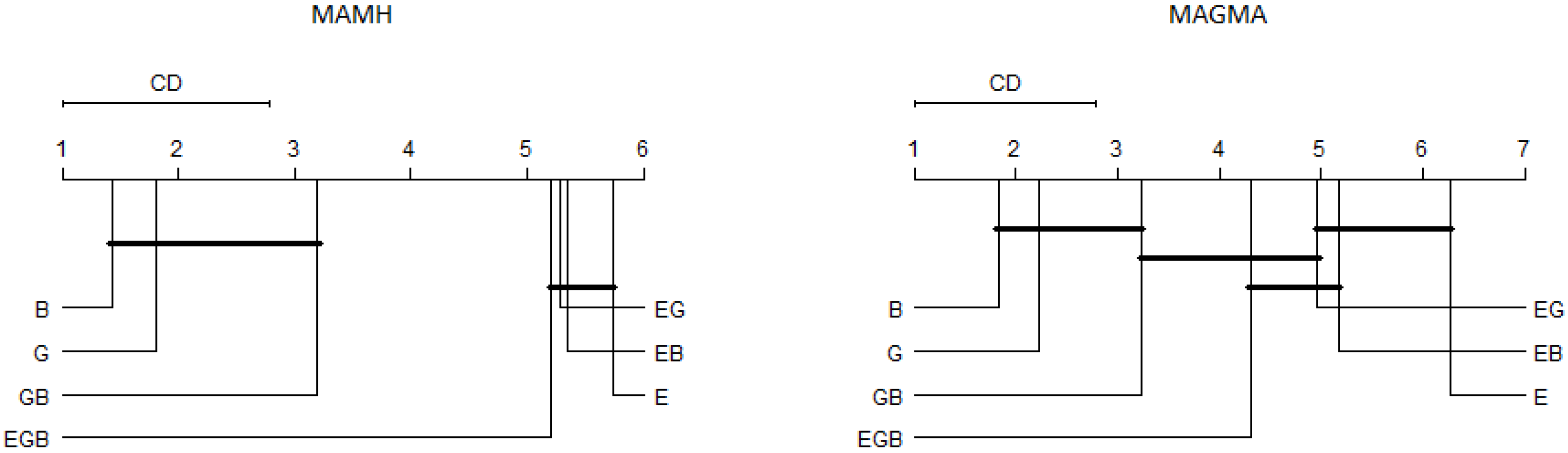Figure 2 presents the results of the critical difference (CD) diagram of The post-hoc Nemenyi test. As we used the error rate as input, the highest values represent the lowest error rates.

In Figure 2, E, EG and EB objectives have provided similar performance, for both MAMH and MAGMA, from a statistical point of view. For MAMH, EGB objective set was similar to E, EB and EG. These results show that the use of the error rate and one diversity measure had a positive effect in the performance of the hybrid architecture. Based on this statistical analysis, we can conclude that there is no best objective set, for both hybrid architectures and any objective set can be selected without strongly deteriorating the performance of the obtained ensembles.

We analyzed the objective sets based solely in the error rate of the obtained ensembles. However, this analysis is not sufficient to evaluate the performance in the multi-objective context. Thus, we then analyzed the performance of the multi-objective cases. As mentioned previously, we first considered the result of the Dominance Ranking to determine a difference between both objective sets. If a statistical difference was not detected at this level, we then applied the Hyper-volume and Binary-$ϵ$ measures. Therefore, a statistical significant difference was detected if a difference was detected at Dominance Ranking or a simultaneous difference in hyper-volume and Binary-$ϵ$ [52].

Table 3. MAMH multi-objective tests.

	EG × EB			EG × EGB
Dataset	DR	H	ϵ	DR	H	ϵ
1	1.0000	0.2222	0.5476	1.0000	0.0079	0.1349
2	1.0000	0.6905	0.5476	1.0000	0.0079	0.2460
3	1.0000	0.0079	0.2222	1.0000	0.0079	0.0952
4	1.0000	0.0079	0.0317	1.0000	0.0079	0.1508
5	1.0000	0.0952	0.0159	1.0000	0.0079	0.8413
6	1.0000	0.1508	0.0476	1.0000	0.0079	0.6905
7	1.0000	0.0079	0.0556	1.0000	0.0079	0.0794
8	1.0000	0.5476	0.0079	1.0000	0.0079	0.2460
9	1.0000	0.0952	0.0079	1.0000	0.0079	0.0317
10	1.0000	0.0952	0.0079	1.0000	0.0079	0.2222
11	1.0000	0.8413	0.1270	1.0000	0.0079	0.6032
12	1.0000	0.0079	0.0317	1.0000	0.0079	0.0952
13	1.0000	0.8413	0.0079	1.0000	0.0079	0.1508
14	1.0000	0.0476	0.0079	1.0000	0.5873	0.5476
15	1.0000	0.8413	0.2222	1.0000	0.0079	1.0000
16	1.0000	0.4206	0.5476	1.0000	0.0079	0.0159
17	1.0000	0.8413	0.2143	1.0000	0.0079	0.3889
18	1.0000	0.0079	0.3095	1.0000	0.0317	0.3413
19	1.0000	0.0952	0.0079	1.0000	0.0079	0.0079
20	1.0000	0.8413	0.1508	1.0000	0.0079	0.2222
21	1.0000	0.0556	0.6905	1.0000	0.0079	0.0317
22	1.0000	0.0079	0.0079	1.0000	0.0079	0.2222
23	1.0000	0.0079	0.1508	1.0000	0.0079	0.9524
24	1.0000	0.0317	0.4127	1.0000	0.3095	0.6667
25	1.0000	0.0079	0.6905	1.0000	0.0556	0.6429
26	1.0000	0.0556	0.6508	1.0000	0.6905	0.6905

DR, Dominance Ranking; H, Hyper-volume; $ϵ$, Binary-$ϵ$.

and

Table 4. MAGMA multi-objective tests.

	EG × EB			EG × EGB
Dataset	DR	H	ϵ	DR	H	ϵ
1	1.0000	0.0079	0.1508	1.0000	0.0079	0.0159
2	1.0000	0.0079	0.8413	1.0000	0.2222	0.4206
3	1.0000	0.0317	0.0317	1.0000	0.0079	0.0079
4	1.0000	0.8413	0.4206	1.0000	0.0079	0.0079
5	1.0000	1.0000	0.4365	1.0000	0.0079	0.0556
6	1.0000	0.0079	0.8413	1.0000	0.0079	0.0556
7	1.0000	0.0556	1.0000	1.0000	0.0079	0.0317
8	1.0000	0.0079	0.8413	1.0000	0.0159	0.0079
9	1.0000	0.2222	0.2222	1.0000	0.0079	0.1508
10	1.0000	0.0079	0.0159	1.0000	0.0079	0.0159
11	1.0000	0.0079	0.0079	1.0000	0.0079	0.0556
12	1.0000	0.0159	0.6905	1.0000	0.0079	0.4206
13	1.0000	0.0159	0.8413	1.0000	0.0079	0.0556
14	1.0000	0.0476	0.0079	1.0000	0.5556	0.0159
15	1.0000	0.0079	0.2857	1.0000	0.0079	0.1508
16	1.0000	0.6905	0.2857	1.0000	0.0556	0.5476
17	1.0000	0.1508	0.6905	1.0000	0.0079	0.6905
18	1.0000	0.0159	0.0317	1.0000	0.0952	0.0317
19	1.0000	0.4206	0.0159	1.0000	0.0079	0.4603
20	1.0000	0.0079	0.5476	1.0000	0.0079	0.0556
21	1.0000	0.0079	0.0952	1.0000	0.0079	0.0317
22	1.0000	0.0079	0.0079	1.0000	0.0317	1.0000
23	1.0000	0.0079	0.2222	1.0000	1.0000	0.6905
24	1.0000	0.4206	1.0000	1.0000	0.0079	0.6429
25	1.0000	0.4206	0.8413	1.0000	0.0317	0.0556
26	1.0000	0.0952	0.2222	1.0000	0.0556	0.3095

DR, Dominance Ranking; H, Hyper-volume; $ϵ$, Binary-$ϵ$.

present the results of the multi-objective context for MAMH and MAGMA, respectively.These tables compare EG to EB and EGB. In addition, the cases highlighted in bold or shaded cells mean that there is a significant statistical difference between the two analyzed objective sets. In this sense, the shaded cells are in favor of EG and the cases highlighted in bold are in favor of the EB or EGB, depending on the comparison.

As shown in Table 3 and Table 4, we detected a few statistical differences. When considering the MAMH algorithm in the comparison of the EG × EB, for instance, there are only four significant differences, being only one in favor of the EG. In the comparison of EG × EGB, there are also four significant differences, being all of them in favor of the EGB. For the MAGMA algorithm, in the comparison of EG × EB, there are six significant differences, being two in favor of EG. In the comparison of EG × EGB, there are seven significant differences, being all of them in favor of EG.

Thus, based on the obtained results, it is clear that the optimizing the EG generates slightly worse results than optimizing EB and EGB, in the MAMH algorithm. However, for MAGMA, it is not clear which objective set, EG, EB or EGB, has the best results, but EG provided slightly better results than EB.

In summary, there is no consensus about the best set of objectives, for both hybrid architectures, since MAGMA obtained the best results with Error (E) and MAMH obtained the best results with Error (E) and Error along with Good diversity (EG). However, these differences were not detected by the statistical test. As the Error objective (E) appeared in both architectures, we used this objective in the comparison analysis with existing ensemble methods. However, before starting this comparative analysis, we compared both MAGMA and MAMH, which is presented in the next subsection.

5.2. The Best Hybrid Architecture

To make a comparative analysis of these two hybrid architectures, we first evaluated the error rate delivered by ensembles obtained by both architectures. To do this, we applied the Signed Rank test, having only two matched populations (MAMH and MAGMA), for each objective set. The result of this test indicates a superior performance of MAGMA over MAMH for E (p-value = 0.0001) and EG (p-value = 0.0056), while superior performance of MAMH over MAGMA for EGB (p-value = 0.00891). For the remaining objective sets, both MAGMA and MAMH provided similar performance, from a statistical point of view. These results show that, if one or two objectives are used, the best architecture is MAGMA, while the best architecture is MAMH when using all three objectives.

To comparative analyze the multi-objective context, we compared both architectures with the same objective sets.

Table 5. MAMH and MAGMA multi-objective tests (same objectives).

	EG			EB			EGB
Dataset	DR	H	ϵ	DR	H	ϵ	DR	H	ϵ
1	0.0476	-	-	1.0000	1.0000	0.9524	1.0000	0.3095	0.1032
2	1.0000	0.0556	0.1190	1.0000	0.4206	1.0000	1.0000	0.0079	0.8889
3	1.0000	0.0079	1.0000	1.0000	0.3095	0.8413	1.0000	0.0159	0.6905
4	1.0000	0.0159	0.0079	1.0000	0.8413	0.5952	1.0000	0.0079	0.4206
5	0.0317	-	-	1.0000	0.4206	0.5476	1.0000	0.0556	0.9365
6	0.4444	0.0079	0.0952	1.0000	0.0317	0.0317	1.0000	0.0079	0.0079
7	1.0000	0.0952	1.0000	0.4444	0.8413	0.1190	1.0000	0.0556	1.0000
8	0.1667	0.1508	0.2222	0.1667	0.0079	0.0397	1.0000	0.0079	0.1746
9	0.1667	0.0079	0.0079	1.0000	1.0000	1.0000	1.0000	0.0079	0.0389
10	1.0000	0.0556	0.1508	1.0000	0.4206	0.2698	1.0000	0.0556	0.6905
11	1.0000	0.0317	0.0079	1.0000	0.6905	0.0079	1.0000	0.0079	0.4206
12	0.0079	-	-	1.0000	0.8413	0.5476	1.0000	0.0952	0.3095
13	1.0000	0.0079	0.0317	1.0000	0.0079	0.0159	1.0000	0.0079	1.0000
14	1.0000	0.2381	0.5476	1.0000	0.2857	1.0000	1.0000	0.8333	0.8492
15	1.0000	0.0079	0.2460	0.4444	0.2222	0.9365	1.0000	0.2222	0.1508
16	1.0000	0.4206	0.2222	0.0476	-	-	1.0000	0.0159	0.0456
17	0.0476	-	-	1.0000	1.0000	0.8889	1.0000	1.0000	0.8016
18	1.0000	0.0952	0.7381	1.0000	0.4603	1.0000	1.0000	0.0952	1.0000
19	1.0000	0.0159	0.8413	1.0000	0.3095	0.1667	1.0000	0.6905	0.2698
20	1.0000	0.0159	0.4206	0.4444	0.0079	0.0556	1.0000	0.0079	0.6905
21	1.0000	0.0079	0.0159	1.0000	0.6905	0.6905	1.0000	0.0079	0.5476
22	1.0000	0.0079	0.4206	1.0000	1.0000	1.0000	1.0000	0.0159	0.4206
23	1.0000	0.8413	0.4206	1.0000	1.0000	1.0000	1.0000	0.0159	0.0238
24	1.0000	0.1508	0.7302	1.0000	0.8413	0.0317	1.0000	0.5476	0.2460
25	1.0000	0.1349	0.7857	0.0476	-	-	1.0000	0.0556	0.2063
26	1.0000	1.0000	1.0000	1.0000	0.8413	0.8413	1.0000	0.6905	0.6905

DR, Dominance Ranking; H, Hyper-volume; $ϵ$, Binary-$ϵ$.

presents the results of the this investigation. Once again, in this table, the cases highlighted in bold represent that a significant statistical difference in favor of MAGMA was detected, and the cases represented by the shaded cells indicate that the significant difference was in favor of MAMH.

In a general perspective, in Table 5, we note a few significant differences between these two architectures. As shown in Table 5, when both architectures use EB, for instance, only five significant differences were detected, of which two favor MAMH and three favor MAGMA. A similar pattern of performance was observed in the EG objective. Thus, when comparing both architectures using two objectives, we can state that both architecture have similar performance, from a statistical point of view. However, when both architectures use EGB, four significant differences were detected, all of them in favor of MAMH. It shows that the use of three objectives had a slightly more positive impact in the performance of MAMH, when compared to MAGMA.

5.3. Comparison with Traditional Metaheuristics

A comparison with traditional optimization techniques was conducted. The parameter setting for all optimization techniques was done using the Irace platform, proposed in [51].

Table 6. The obtained results of all optimization techniques, using the classification error (E) as objective.

Dataset	MAMH	MAGMA	GRASP	Genetic	ACO	PSO
1	0.1154	0.1130	0.1070	0.1412	0.1202	0.1082
2	0.0048	0.0000	0.0048	0.0122	0.0090	0.0000
3	0.2354	0.2316	0.2538	0.2614	0.2484	0.2724
4	0.2000	0.1742	0.2080	0.2404	0.2136	0.1844
5	0.2134	0.2000	0.2226	0.2454	0.2336	0.2058
6	0.1182	0.1136	0.1260	0.1316	0.1304	0.1348
7	0.0620	0.0504	0.0772	0.0878	0.0826	0.0504
8	0.0046	0.0026	0.0072	0.0134	0.0090	0.0100
9	0.2290	0.2116	0.2250	0.2594	0.2422	0.2000
10	0.0262	0.0218	0.0210	0.0418	0.0226	0.0232
11	0.0452	0.0444	0.0450	0.0712	0.0460	0.0544
12	0.1640	0.1600	0.1800	0.1980	0.1930	0.1680
13	0.0048	0.0048	0.0648	0.0166	0.0112	0.0190
14	0.0000	0.0000	0.0000	0.0000	0.0000	0.0000
15	0.0180	0.0080	0.0110	0.0300	0.0160	0.0122
16	0.0498	0.0478	0.0576	0.0570	0.0618	0.0654
17	0.2560	0.2430	0.2660	0.2726	0.2800	0.2418
18	0.0180	0.0040	0.0200	0.0340	0.0220	0.0060
19	0.0096	0.0130	0.0200	0.0190	0.0436	0.0184
20	0.0078	0.0046	0.0080	0.0202	0.0092	0.0126
21	0.1520	0.1424	0.1630	0.1596	0.1860	0.1666
22	0.0000	0.0000	0.0068	0.0000	0.3200	0.0100
23	0.0000	0.0000	0.0170	0.0000	0.0734	0.0000
24	0.0176	0.0194	0.0204	0.0178	0.0000	0.0186
25	0.0064	0.0072	0.0040	0.0096	0.0088	0.0072
26	0.0114	0.0144	0.0130	0.0166	0.0000	0.0164

presents the error rate of the hybrid architectures, along with four well-known metaheuristic algorithms: ACO (Ant Colony Optimization), PSO (Particle Swarm Optimization), GA (Genetic Algorithm) and GRASP. As already explained, the error rates were obtained when using ensemble system obtained by using only the Error objective (E), for simplicity. Additionally, the bold numbers represent the lowest error rate, for each dataset.

When analyzing the results in this table, we could observe that the hybrid architectures provided more accurate ensembles (bold numbers), for the majority of datasets. We then applied the Friedman test, obtaining a p-value $\le 0.0001$. In other words, the statistical test detected a significant difference in performance of all optimization techniques. We then applied the pairwise post-hoc Nemenyi test and the results of this test are presented in Figure 3.

The results in Figure 3 corroborate the results in Table 6, showing that the superiority in performance of the hybrid architectures over the traditional metaheuristic is significant, from a statistical point of view.

5.4. Comparison with Existing Ensemble Generation Techniques

In the final part of the analysis, a comparative analysis with existing ensemble generation techniques was conducted. First, we compared the results of the hybrid metaheuristic with some traditional ensemble generation techniques: random selection, bagging and boosting (more details about these methods can be found [53]). The random selection generates a heterogeneous committee by randomly choosing individual classifiers. In addition, it has a feature selection step, in which a random selection of around 70% of the feature set is selected, for each individual classifier. Bagging and Boosting are designed using a decision tree as base classifiers (k-NN and Naive Bayesian were analyzed but DT provided the best overall result). One hundred iterations were used in both methods since it provided the overall best performance. The results of this analysis are presented in

Table 7. The error rate of the hybrid architectures and three traditional ensemble generation techniques.

Dataset	MAMH	MAGMA	Boosting	Bagging	Random
1	0.1154	0.1130	0.1696	0.1497	0.1521
2	0.0048	0.0000	0.0270	0.0270	0.0281
3	0.2354	0.2316	0.3018	0.3255	0.3301
4	0.2000	0.1742	0.2773	0.3031	0.2876
5	0.2134	0.2000	0.2849	0.3075	0.3123
6	0.1182	0.1136	0.1693	0.1704	0.1562
7	0.0620	0.0504	0.1265	0.1303	0.1226
8	0.0046	0.0026	0.0267	0.0246	0.0524
9	0.2290	0.2116	0.3010	0.2981	0.3076
10	0.0262	0.0218	0.0616	0.0559	0.0637
11	0.0452	0.0444	0.0833	0.0696	0.0685
12	0.1640	0.1600	0.2258	0.2313	0.2354
13	0.0048	0.0048	0.0794	0.0763	0.1713
14	0.0000	0.0000	0.0193	0.0140	0.0281
15	0.0180	0.0080	0.0707	0.0728	0.0878
16	0.0498	0.0478	0.0869	0.0789	0.1054
17	0.2560	0.2430	0.2945	0.3022	0.3077
18	0.0180	0.0040	0.0693	0.0495	0.0554
19	0.0096	0.0130	0.0415	0.0262	0.0219
20	0.0078	0.0046	0.0399	0.0298	0.0235
21	0.1520	0.1424	0.1993	0.1870	0.2142
22	0.0000	0.0000	0.0817	0.1217	0.1683
23	0.0000	0.0000	0.0617	0.0300	0.1000
24	0.0176	0.0194	0.0230	0.0251	0.0244
25	0.0064	0.0072	0.0250	0.0206	0.0286
26	0.0114	0.0144	0.0379	0.0364	0.0503

.

In this table, we can observe that the hybrid architectures provided more accurate ensembles than traditional ensemble generation techniques, for all datasets. We then applied the Friedman test, obtaining a p-value $\le 0.0001$. In other words, the statistical test detected a significant difference in performance of all ensemble generation techniques. The p-vales of the post-hoc Nemenyi test, comparing each pair of techniques are presented in

Table 8. Post-hoc Nemenyi tests for classical ensemble techniques.

x	Boosting	Bagging	Random
MAMH	<0.0001	<0.0001	<0.0001
MAGMA	<0.0001	<0.0001	<0.0001

. In this table, the shaded cells indicate a significant difference in favor of the hybrid architecture.

The Nemenyi test showed that the superiority of the hybrid architectures was statistically significant. The results obtained are promising, showing that the hybrid architectures proposed in this paper are able to provide accurate ensembles, better than well-established ensemble generation techniques.

Once the comparison with traditional ensemble techniques was conducted, a comparison with recent and promising ensemble techniques was conducted. We selected four ensemble generation techniques: Random Forest (it has largely been used in the ensemble community), XGBoost (a more powerful version of Boosting, proposed in [54]) and P2-SA and P2-WTA [33] (two versions of a multi-objective algorithm for selecting members for an ensemble system).

The Random Forest implementation was exported from WEKA package and we used 100–1000 random trees, depending on the dataset. The XGBoost implementation was the one indicated by the authors in [54] and we used 100–500 gbtrees. However, for P2-SA and P2-WTA, we used the original results, provided in [33]. Thus, this comparative analysis used a different group of datasets, since they are the ones used in [33] and are publicly available. All datasets were also extracted from UCI repository [42].

Table 9. The error rate of the hybrid architectures and four recent ensemble techniques.

Dataset	MAMH	MAGMA	RandomForest	XGBoost	P2-SA [33]	P2-WTA [33]
Autos	0.061	0.076	0.148	0.171	0.337	0.331
Balance	0.078	0.078	0.194	0.120	0.080	0.085
German	0.197	0.193	0.243	0.249	0.283	0.257
Heart	0.084	0.086	0.168	0.150	0.174	0.178
Horse	0.201	0.211	0.305	0.312	0.364	0.366
Liver	0.213	0.212	0.286	0.290	0.307	0.301
PageBl	0.022	0.021	0.025	0.028	0.062	0.058
Pima	0.198	0.198	0.228	0.267	0.245	0.240
SatImage	0.067	0.073	0.081	0.079	0.143	0.140
Segment	0.011	0.010	0.018	0.012	0.063	0.061
Vehicle	0.235	0.231	0.248	0.220	0.235	0.238

presents the error rates of all six ensemble methods. Once again, the bold numbers represents the ensemble method with the lowest error rate for a dataset.

As can be seen in Table 9, the lowest error rate was almost always obtained by a hybrid metaheuristic, with both architectures having five bold numbers. The only exception was the Vehicle dataset, in which the lowest error rate was obtained by XGBoost. We then applied the Friedman test, obtaining a p-value = 0.002, when comparing MAMH, MAGMA, Random Forest and XGBoost. In other words, the statistical test detected a significant difference in performance of these four ensemble generation techniques. It is important to highlight that P2-SA and P2-WTA were not included in the statistical test since we only had access to the mean accuracy and standard deviation of these techniques, not allowing the application of the statistical test. The Nemenyi test was then applied and it showed that MAGMA and MAMH were statistically superior to Random Forest and XGBoost.

Our final analysis was related to the time processing for all four implemented ensemble techniques. Once again, the time processing, measured in seconds, was not provided in [33] and we could not include P2-SA and P2-WTA processing time values in this comparison.

Table 10. The processing time (s) of the hybrid architectures and two ensemble techniques.

Dataset	MAMH	MAGMA	RandomForest	XGBoost
Balance	59.6	58.8	17.6	12.2
Heart	292.3	211.5	80.9	70.4
Segment	3740.7	1509.7	347.5	115.3
Autos	762.0	751.2	144.1	115.5
Liver	825.9	712.1	120.9	128.5
Pima	1027.5	1007.1	324.9	335.1
Horse	953.6	885.4	234.3	284.6
Vehicle	820.3	275.7	381.2	356.6
German	1317.9	1265.7	158.4	130.5
PageBl	3789.8	2096.6	432.2	329.0
SatImage	10,981.3	7206.8	4019.5	1452.7

presents the processing time of all four ensemble methods.

In fact, the hybrid metaheuristics need more processing time than Random Forest and XGBoost. We believe that the use of ensemble accuracy as an objective in MAMH and MAGMA is a complex function, leading to higher processing time than the other two ensemble methods. The use of less complex objectives as well as the use of techniques to optimize the search process will cause a decrease in the processing time and this is the subject of an on-going research.

In summary, the results in Table 7 and Table 9 show that the use of hybrid metaheuristics provided more accurate ensembles than traditional and recent ensemble techniques. However, in Table 10, we can observe that these techniques need more processing time.

5.5. An Analysis of Obtained Results

As can be observed, various results are presented in the previous sections. In this section, we assess and explain the obtained results. Seven different objective sets were evaluated, for both proposed metaheuristics. As a result of this analysis, we state that the application of the diversity measures as objective function in the mono-objective algorithms led to a decrease in the accuracy of the classifier ensembles for both hybrid architectures. In a way, it was an expected result since it is known that the use of a diversity measure on its own would not surpass the performance of the error rate in the design of accurate classifier ensembles. However, it is important to highlight that the inclusion of one diversity measure, along with error rate, can have a positive affect in the search for accurate ensemble systems, mainly for MAMH. Additionally, the obtained results show that the best result for MAMH was obtained using a different objective set (EG), when compared to MAGMA (the best result was obtained with E). In addition, we could observe that MAMH provided the best results in the multi-objective context, while MAGMA in the mono-objective context. This analysis showed that the choice of the objective set is an optimization-based selection.

In the second analysis of this paper, an analysis of the hybrid architectures was performed; we can conclude that MAGMA provided slightly better performance than MAMH in the mono-objective context. For the multi-objective context, both architectures have similar performance, with MAMH having better performance than MAGMA when using three objectives. Once again, this might be an indication that MAGMA is the most appropriate technique in the mono-objective context, while MAMH is the best one for the multi-objective context. We believe that the dynamic aspect of MAMH, changing the learning strategy more often than MAGMA had been more efficient when using more than one objective to optimize. In other words, this caused a decrease in performance in the mono-objective context and an increase in the multi-objective context.

In the third part of this analysis, the performance of the hybrid architectures was analyzed in relation to the traditional algorithms. It is natural to assume that hybrid algorithms perform better than traditional algorithms since their strategy is to use the synergy among components of different techniques to generate better results. This improvement was detected by the statistical test.

Finally, we compared the performance of the hybrid architectures to traditional ensemble generation techniques, such as Boosting and Bagging. In addition, we compared them with recent ensemble techniques: XGBoost, Random Forest and P2-SA and P2-WTA [33]. The obtained results showed that the hybrid architectures proposed in this paper are able to provide accurate ensembles, better than well-established and recent ensemble generation techniques.

6. Final Remarks

The focus of this work was the use of hybrid optimization metaheuristics to generate accurate ensembles. Therefore, we present two different hybrid architectures, MAMH and MAGMA, that were adapted to be applied to the automatic design of ensemble system, in both mono- and multi-objective contexts.

To evaluate the performance of the hybrid architecture in the design of accurate ensembles, an empirical analysis was conducted. Through this analysis, we could observe that MAMH provided the best results in the multi-objective context, while MAGMA in the mono-objective context. This analysis showed that the choice of the objective set is a optimization-based selection. In comparison with traditional optimization techniques, the hybrid architectures provided more accurate ensemble than the traditional optimization techniques, for the majority of the analyzed cases.

Finally, when compared to recent ensemble generation techniques, the hybrid architectures were also able to provide more accurate ensembles than well-established ensemble generation techniques. However, in this comparative analysis, we also evaluated the processing time and we observed that the hybrid metaheuristics need more processing time than Random Forest and XGBoost. We believe that the use of ensemble accuracy as an objective in the optimization technique makes the processing time of MAMH and MAGMA higher than the other two ensemble methods. The use of less complex objectives as well as the use of techniques to optimize the search process will decrease the processing time, and this is the subject of an on-going research.

References

- Mitchell, T. Machine Learning; McGraw Hill: New York, NY, USA, 1997. [Google Scholar]
- Kuncheva, L.I. Combining Pattern Classifiers: Methods and Algorithms; Wiley: Hoboken, NJ, USA, 2004. [Google Scholar]
- Brown, G.; Wyatt, J.; Harris, R.; Yao, X. Diversity creation methods: A survey and categorisation. Inf. Fusion 2005, 6, 5–20. [Google Scholar] [CrossRef]
- Ren, Y.; Zhang, L.; Suganthan, P.N. Ensemble Classification and Regression—Recent Developments, Applications and Future Directions. IEEE Comput. Intell. Mag. 2016, 11, 41–53. [Google Scholar] [CrossRef]
- Woźniak, M.; Graña, M.; Corchado, E. A survey of multiple classifier systems as hybrid systems. Inf. Fusion 2014, 16, 3–17. [Google Scholar] [CrossRef]
- Boussaïd, I.; Lepagnot, J.; Siarry, P. A survey on optimization metaheuristics. Inf. Sci. 2013, 237, 82–117. [Google Scholar] [CrossRef]
- Souza, G.; Goldbarg, E.; Goldbarg, M.; Canuto, A. A multiagent approach for metaheuristics hybridization applied to the traveling salesman problem. In Proceedings of the 2012 Brazilian Symposium on Neural Networks, Curitiba, Paraná, Brazil, 20–25 October 2012; pp. 208–213. [Google Scholar]
- Tiejun, Z.; Yihong, T.; Lining, X. A multi-agent approach for solving traveling salesman problem. Wuhan Univ. J. Nat. Sci. 2006, 11, 1104–1108. [Google Scholar] [CrossRef]
- Xie, X.-F.; Liu, J. Multiagent optimization system for solving the traveling salesman problem (tsp). IEEE Trans. Syst. Man Cybern. Part B 2009, 39, 489–502. [Google Scholar]
- Fernandes, F.; Souza, S.; Silva, M.; Borges, H.; Ribeiro, F. A multiagent architecture for solving combinatorial optimization problems through metaheuristics. In Proceedings of the IEEE International Conference on Systems, Man and Cybernetics, San Antonio, TX, USA, 11–14 October 2009; pp. 3071–3076. [Google Scholar]
- Malek, R. An agent-based hyper-heuristic approach to combinatorial optimization problems. In Proceedings of the IEEE International Conference on Intelligent Computing and Intelligent Systems (ICIS), Xiamen, China, 29–31 October 2010; pp. 428–434. [Google Scholar]
- Milano, M.; Role, A. MAGMA: A multiagent architecture for metaheuristics. IEEE Trans. Syst. Man Cybern. Part B 2004, 34, 925–941. [Google Scholar] [CrossRef]
- Brown, G.; Kuncheva, L. “Good” and “bad” diversity in majority vote ensembles. In Multiple Classifier Systems; Springer: Berlin/Heidelberg, Germany, 2010; pp. 124–133. [Google Scholar]
- Feitosa Neto, A.A.; Canuto, A.M.P.; Xavier-Júnior, J.C. A multi-agent metaheuristic hybridization to the automatic design of ensemble systems. In Proceedings of the 2017 International Joint Conference on Neural Networks (IJCNN 2017), Anchorage, AK, USA, 14–19 May 2017. [Google Scholar]
- Feitosa Neto, A.; Canuto, A.M.P. An exploratory study of mono- and multi-objective metaheuristics to ensemble of classifiers. Appl. Intell. 2018, 48, 416–431. [Google Scholar] [CrossRef]
- Feurer, M.; Klein, A.; Eggensperger, K.; Springenberg, J.; Blum, M.; Hutter, F. Efficient and Robust Automated Machine Learning. Adv. Neural Inf. Process. Syst. 2015, 28, 2962–2970. [Google Scholar]
- Kordík, P.; Černý, J.; Frýda, T. Discovering Predictive Ensembles for Transfer Learning and Meta-Learning. Mach. Learn. 2018, 107, 177–207. [Google Scholar] [CrossRef]
- Kotthoff, L.; Thornton, C.; Hoos, H.; Hutter, F.; Leyton-Brown, K. Auto-WEKA 2.0: Automatic model selection and hyperparameter optimization in WEKA. J. Mach. Learn. Res. 2017, 18, 826–830. [Google Scholar]
- Albukhanajer, W.A.; Jin, Y.; Briffa, J.A. Classifier ensembles for image identification using multi-objective Pareto features. Neurocomputing 2017, 238, 316–327. [Google Scholar] [CrossRef]
- Wistuba, M.; Schilling, N.; Schmidt-Thieme, L. Automatic Frankensteining: Creating Complex Ensembles Autonomously. In Proceedings of the 2017 SIAM International Conference on Data Mining, Houston, TX, USA, 27–29 April 2017; pp. 741–749. [Google Scholar]
- Zhang, L.; Srisukkham, W.; Neoh, S.C.; Lim, C.P.; Pandit, D. Classifier ensemble reduction using a modified firefly algorithm: An empirical evaluation. Expert Syst. Appl. 2018, 93, 395–422. [Google Scholar] [CrossRef]
- Nascimento, D.S.C.; Canuto, A.M.P.; Coelho, A.L.V. An Empirical Analysis of Meta-Learning for the Automatic Choice of Architecture and Components in Ensemble Systems. In Proceedings of the 2014 Brazilian Conference on Intelligent Systems, Sao Paulo, Brazil, 18–22 October 2014; pp. 1–6. [Google Scholar]
- Khan, S.A.; Nazir, M.; Riaz, N. Optimized features selection for gender classication using optimization algorithms. Turk. J. Electr. Eng. Comput. Sci. 2013, 21, 1479–1494. [Google Scholar] [CrossRef]
- Palanisamy, S.; Kanmani, S. Classifier Ensemble Design using Artificial Bee Colony based Feature Selection. IJCSI Int. J. Comput. Sci. 2012, 9, 522–529. [Google Scholar]
- Wang, L.; Ni, H.; Yang, R.; Pappu, V.; Fenn, M.B.; Pardalos, P.M. Feature selection based on meta-heuristics for biomedicine. Opt. Methods Softw. 2014, 29, 703–719. [Google Scholar] [CrossRef]
- Zhang, T.; Dai, Q.; Ma, Z. Extreme learning machines’ ensemble selection with GRASP. Appl. Intell. 2015, 43, 439–459. [Google Scholar] [CrossRef]
- Liu, Z.; Dai, Q.; Liu, N. Ensemble selection by GRASP. Appl. Intell. 2014, 41, 128–144. [Google Scholar] [CrossRef]
- Acosta-Mendoza, N.; Morales-Reyes, A.; Escalante, H.; Gago-Alonso, A. Learning to Assemble Classifiers via Genetic Programming. Int. J. Pattern Recognit. Artif. Intell. 2014, 28, 1460005. [Google Scholar] [CrossRef]
- Oh, D.-Y.; Brian Gray, J. GA-Ensemble: A genetic algorithm for robust ensembles. Comput. Stat. 2013, 28, 2333–2347. [Google Scholar] [CrossRef]
- Chen, Y.; Zhao, Y. A novel ensemble of classifiers for microarray data classification. Appl. Soft Comput. 2008, 8, 1664–1669. [Google Scholar] [CrossRef]
- Lysiak, R.; Kurzynski, M.; Woloszynski, T. Optimal selection of ensemble classifiers using measures of competence and diversity of base classifiers. Neurocomputing 2014, 126, 29–35. [Google Scholar] [CrossRef]
- Mao, L.C.S.; Jiao, L.; Xiong, S.G. Greedy optimization classifiers ensemble based on diversity. Pattern Recognit. 2011, 44, 1245–1261. [Google Scholar] [CrossRef]
- Fernández, J.C.; Cruz-Ramírez, M.; Hervás-Martínez, C. Sensitivity Versus Accuracy in Ensemble Models of Artificial Neural Networks from Multi-objective Evolutionary Algorithms. Neural Comput. Appl. 2016. [Google Scholar] [CrossRef]
- Qasem, S.N.; Shamsuddin, S.M.; Hashim, S.Z.; Darus, M.; Al-Shammari, E. Memetic multiobjective particle swarm optimization-based radial basis function network for classificationproblems. Inf. Sci. 2013, 239, 165–190. [Google Scholar] [CrossRef]
- Salman, I.; Ucan, O.; Bayat, O.; Shaker, K. Impact of Metaheuristic Iteration on Artificial Neural Network Structure in Medical Data. Processes 2018, 6, 57. [Google Scholar] [CrossRef]
- Bertolazzi, P.; Felici, G.; Festa, P.; Fiscon, G.; Weitschek, E. Integer programming models for feature selection: New extensions and a randomized solution algorithm. Eur. J. Oper. Res. 2016, 250, 389–399. [Google Scholar] [CrossRef]
- Festa, P.; Resende, M.G.C. GRASP: Basic components and enhancements. Telecommun. Syst. 2011, 46, 253–271. [Google Scholar] [CrossRef]
- Fiscon, G.; Weitschek, E.; Cella, E.; Presti, A.L.; Giovanetti, M.; Babakir-Mina, M.; Ciotti, M.; Ciccozzi, M.; Pierangeli, A.; Bertolazzi, P.; et al. MISSEL: A method to identify a large number of small species-specific genomic subsequences and its application to viruses classification. BioData Min. 2016, 9, 38. [Google Scholar] [CrossRef] [PubMed]
- Blum, C.; Puchinger, J.; Raidl, G.R.; Roli, A. Hybrid metaheuristics in combinatorial optimization: A survey. Appl. Soft Comput. 2011, 11, 4135–4151. [Google Scholar] [CrossRef]
- Demšar, J. Statistical comparisons of classifiers over multiple datasets. J. Mach. Learn. Res. 2006, 7, 1–30. [Google Scholar]
- Dheeru, D.; Taniskidou, E.K.; UCI Machine Learning Repository. University of California, Irvine, School of Information and Computer Sciences. 2017. Available online: http://archive.ics.uci.edu/ml (accessed on 23 October 2018).
- Monti, S.; Tamayo, P.; Mesirov, J.; Golub, T. Consensus clustering—A resampling-based method for class discovery and visualization of gene expression microarray data. Mach. Learn. 2003, 52, 91–118. [Google Scholar] [CrossRef]
- Feo, T.A.; Resende, M.G.C. Greedy randomized adaptive search procedures. J. Glob. Opt. 1995, 6, 109–133. [Google Scholar] [CrossRef]
- Gendreau, M.; Potvin, J. Handbook of Metaheuristics, 2nd ed.; Springer: Berlin, Germany, 2010. [Google Scholar]
- Glover, F. Tabu Search and Adaptive Memory Programming—Advances, Applications and Challenges. In Interfaces in Computer Sciences and Operations Research; Kluwer Academic Publishers: Norwell, MA, USA, 1996; pp. 1–75. [Google Scholar]
- Goldberg, D.E. Genetic Algorithms in Search, Optimization and Machine Learning; Addison-Wesley: Berkeley, CA, USA, 1989. [Google Scholar]
- Deb, K.; Pratap, A.; Agarwal, S.; Meyarivan, T. A fast and elitist multiobjective genetic algorithm: NSGA-II. IEEE Trans. Evol. Comput. 2002, 6, 182–197. [Google Scholar] [CrossRef]
- Dorigo, M. Optimization, Learning and Natural Algorithms. Ph.D. Thesis, Dipartimento di Elettronica, Politecnico di Milano, Italy, 1992. [Google Scholar]
- Lee, K.Y.; El-Sharkawi, M.A. Modern Heuristic Optimization Techniques—Theory and Applications to Power Systems; Wiley-Interscience: Hoboken, NJ, USA, 2008. [Google Scholar]
- Goldbarg, E.F.G.; Goldbarg, M.C.; de Souza, G.R. Particle Swarm Optimization Algorithm for the Traveling Salesman Problem; Springer: Berlin, Germany, 2006; pp. 99–110. [Google Scholar]
- López-Ibáñez, M.; Dubois-Lacoste, J.; Cáceres, L.P.; Stützle, T.; Birattari, M. The irace package: Iterated Racing for Automatic Algorithm Configuration. Oper. Res. Perspect. 2016, 3, 43–58. [Google Scholar] [CrossRef]
- Knowles, J.D.; Thiele, L.; Zitzler, E. A tutorial on the performance assessment of stochastic multiobjective optimizers. In Computer Engineering and Networks Laboratory (TIK); ETH Zurich: Zürich, Switzerland, 2006. [Google Scholar]
- Witten, I.H.; Frank, E. Data Mining—Pratical Learning Tools and Techniques, 2nd ed.; Morgan Kaufmann: Burlington, MA, USA, 2005. [Google Scholar]
- Chen, T.; Guestrin, C. XGBoost: A Scalable Tree Boosting System. arXiv, 2016; arXiv:160302754C. [Google Scholar]
© 2018 by the authors. Licensee MDPI, Basel, Switzerland. This article is an open access article distributed under the terms and conditions of the Creative Commons Attribution (CC BY) license (http://creativecommons.org/licenses/by/4.0/).