Rough Set-Probabilistic Neural Networks Fault Diagnosis Method of Polymerization Kettle Equipment Based on Shuffled Frog Leaping Algorithm

Abstract

In order to realize the fault diagnosis of the polyvinyl chloride (PVC) polymerization kettle reactor, a rough set (RS)–probabilistic neural networks (PNN) fault diagnosis strategy is proposed. Firstly, through analysing the technique of the PVC polymerization reactor, the mapping between the polymerization process data and the fault modes is established. Then, the rough set theory is used to tackle the input vector of PNN so as to reduce the network dimensionality and improve the training speed of PNN. Shuffled frog leaping algorithm (SFLA) is adopted to optimize the smoothing factor of PNN. The fault pattern classification of polymerization kettle equipment is to realize the nonlinear mapping from symptom set to fault set according to the given symptom set. Finally, the fault diagnosis simulation experiments are conducted by combining with the industrial on-site historical datum of polymerization kettle, and the results show that the RS–PNN fault diagnosis strategy is effective.

1. Introduction

Polyvinyl chloride (PVC) is one of the five largest thermoplastic synthetic resins, and its production is second only to polyethylene (PE) and polypropylene (PP). PVC is a kind of general colophony, which is high in quality and is widely used. It has good mechanical and chemical properties, and it is corrosion-resistant and difficult to burn [1]. With vinyl chloride monomer (VCM) as a raw material, the suspension method to produce polyvinyl chloride (PVC) resin is a kind of typical batch chemical production process. PVC polymerization process is a complex control system with multivariable, uncertain, nonlinear, and strong coupling. Polymerization kettle is the key equipment of the PVC production process, where vinyl chlorides go on the polymerization reaction to generate polyvinyl chloride [1]. Whether the polymerization kettle can run steadily is directly related to the working conditions of the PVC production device. On the other hand, the motor, reducer, and machine seal are key equipment to ensure that the polymerization kettle device runs normally. Failure to work will cause serious losses in the PVC polymerizing process [2]. Therefore, the earlier diagnosis of the fault type and location of the polymerization kettle can prevent the huge economic losses which are caused by the parking of the polymerization kettle, which is important for improving the product quality and reducing the production costs [3,4].

Probabilistic neural network (PNN) is a kind of feed-forward neural networks based on Bayesian minimum risk criteria (Bayesian decision theory), which has the features of simple structure, quick training speed, good network fault tolerance and strong pattern classification ability. The advantage is that a linear learning algorithm is used to realize the nonlinear training. PNN has been widely used in many fields, such as fault diagnosis, data classification and processing, image processing, pattern recognition, and so on [5,6,7,8,9]. The combination of the artificial fish-swam algorithm and the probabilistic neural network was investigated for the steam turbine fault diagnosis applications [10]. The artificial fish swarm algorithm is adopted to train the probabilistic neural network. The correct diagnosis rate based on steam turbine fault diagnosis is 87%, while the one based on fish-swarm optimized network is 96%. Reference [11] proposed a new algorithm for detecting faults in an electrical power transmission system, using discrete wavelet transform (DWT) and probabilistic neural network (PNN). Various cases based on Thailand’s electricity transmission systems are studied to verify the validity of the proposed technique. The result shows that the algorithm is capable of performing the fault locations with accuracy. Reference [12] proposed a novel fault diagnosis method based on pulse coupled neural network (PCNN) and probability neural network (PNN). A PCNN combined with roundness method is used to extract the feature vector of shaft orbit. Further, the PNN is used to train the feature vectors and classify the vibration fault. By comparison with the back-propagation (BP) network and radial-basic function (RBF) network, the experimental result indicated the proposed approach achieved fast and efficient fault diagnosis. Reference [13] introduced two different probabilistic neural network (PNN) structures for malignant mesothelioma’s disease diagnosis. The PNN results were compared with the results of the multilayer and learning vector quantization neural networks focusing on MM’s disease diagnosis and using same database. It was observed the PNN is the best classification with 96.30% accuracy obtained via three-fold cross-validation.

PNN has strong fault tolerant ability and adaptive ability, but its performance depends on the selection of network parameters. At present, there is a bottleneck problem in the research on the mechanism of PNN neural network: which is to extract the smooth factor σ reflecting the whole sample space under the limited pattern samples. Too small σ will result in the isolation role for individual training samples, in essence, the nearest neighbor classifier. Too bigger σ will not completely distinguish the details and obtain the ideal classification effect for different classifications with no clear boundaries, which is the same as the linear classifier in essence. Therefore, how to determine the appropriate parameter σ is a key problem of the probabilistic neural network.

If the training pattern samples have been determined, the numerical variety of the smoothing factor σ affects the correlation degree among pattern samples and the change of probability density distribution function. At present, the estimation of the smoothing factor σ is mainly obtained by the empirical estimation or the clustering method based on very limited samples, which does not represent the spatial probability characteristic fully.

Shuffled frog leap algorithm (SFLA) is a population-based heuristic cooperative swarm intelligent search algorithm. SFLA adopts the meta-heuristic algorithm based on swarm intelligence to solve the combinatorial optimization problems, which is based on the meme evolution of the individuals in the population and global information exchange of the memes. SFLA combines the advantages of the genetic-based memetic algorithm (MA) and particle swarm optimization (PSO) with foraging behaviors of the population, such as simple concept, few parameters, quick calculation speed, global optimization capability, and easy to implement features. So, the shuffled frog leaping algorithm (SFLA) is used to optimize the smoothing factor σ in order to accelerate the convergence speed of the algorithm, increase the fault diagnosis accuracy of PNN. On the other hand, the proposed SFLA is compared with genetic algorithm (GA). The simulation results show the advantages of the adopted SFLA.

In this paper, for the fault diagnosis of the large-scale PVC polymerization reactor, a fault diagnosis strategy of the polymerization reactor based on rough set–probabilistic neural networks optimized by shuffled frog leaping algorithm is proposed. The simulation results show the effectiveness of the proposed fault diagnosis strategy. The paper is organized as follows. In Section 2, the technique flowchart of the PVC polymerization process is introduced. The probabilistic neural network is presented in Section 3. In Section 4, the rough set-probabilistic neural network based on shuffled frog leaping algorithm is introduced. The simulation experiments and results analysis are introduced in detail in Section 5. Finally, the conclusion illustrates the last part.

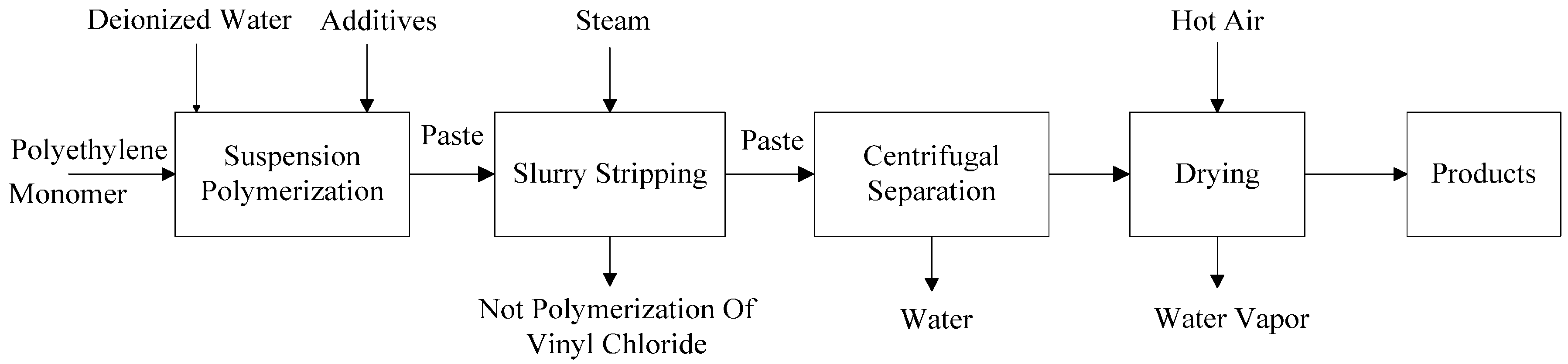
2. Polyvinyl Chloride (PVC) Polymerization Process

2.1. Technique Flowchart

Four methods (suspension polymerization, emulsion polymerization, bulk polymerization and liquor polymerization) are usually used in the PVC polymerization process. Among them, the suspension polymerization is one of the most widely used methods, whose technique flowchart is shown in Figure 1 [2]. Firstly, the suspending agent and deionizer water are fed into the polymerization kettle. Then, the initiator is added and the polymerization kettle is sealed. The oxygen in the material and the air in the polymerization kettle are removed by vacuum. After adding the monomer vinyl chloride, the polymerization kettle starts to be stirred and heated. The temperature must be kept around 50 °C and the pressure is maintained to 0.89~1.23 MPa. When the conversion ratio reaches about 70%, the pressure is reduced gradually. When the pressure drops to 0.13~0.48 MPa, the polymerization kettle reaction is terminated. After the transformation is completed, the vinyl chloride monomer that does not react is pulled out. The remaining slurry is carried out in the stripping process to recycle the pulled out vinyl chloride monomer. Then, a centrifugal separation is used on the stripped slurry. When the water content reaches around 25%, the slurry is put into the dryer until the water content reaches about 0.3%~0.4%. The typical technique process of PVC polymerization kettle is shown in Figure 2 [3].

Figure 1. Flow chart of suspension polymerization.

Figure 1. Flow chart of suspension polymerization.

Figure 2. Technique flowchart of polymerization kettle.

Figure 2. Technique flowchart of polymerization kettle.

In the PVC polymerization process, various raw materials and additives are added to the reaction kettle, which are full evenly dispersed under the mixing action. Then, the suitable amounts of the initiators are added to the kettle and start to react. The cooling water is constantly poured into the jacket and baffle of reaction kettle to remove the reaction heat. The reaction will be terminated and the final products are obtained when the conversion ratio of the vinyl chloride (VCM) reaches a certain value and a proper pressure drop appears. Finally, after the reaction is completed and VCM contained in slurry separated by the stripping technique, the remaining slurry is fed into the drying process for dewatering and drying.

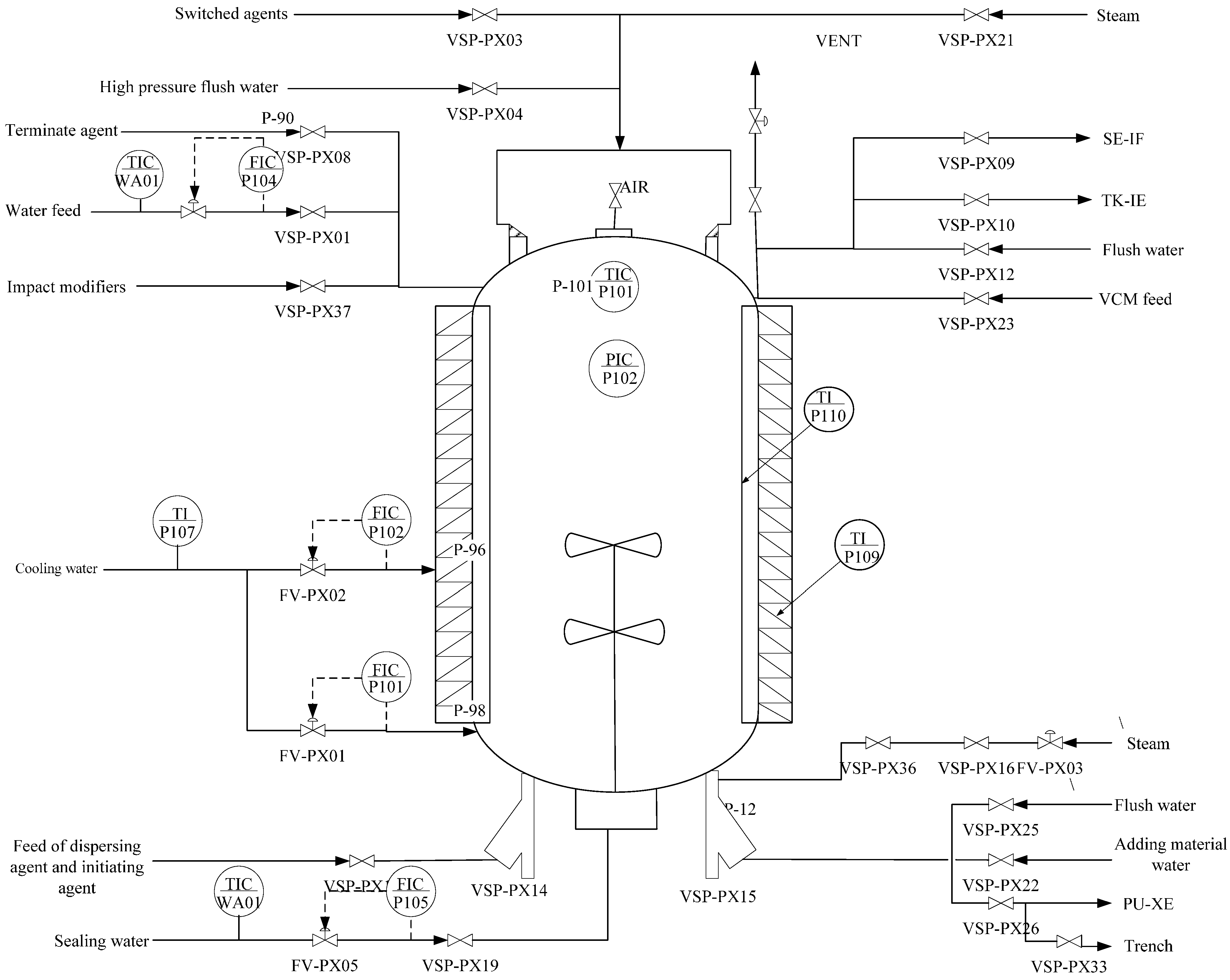
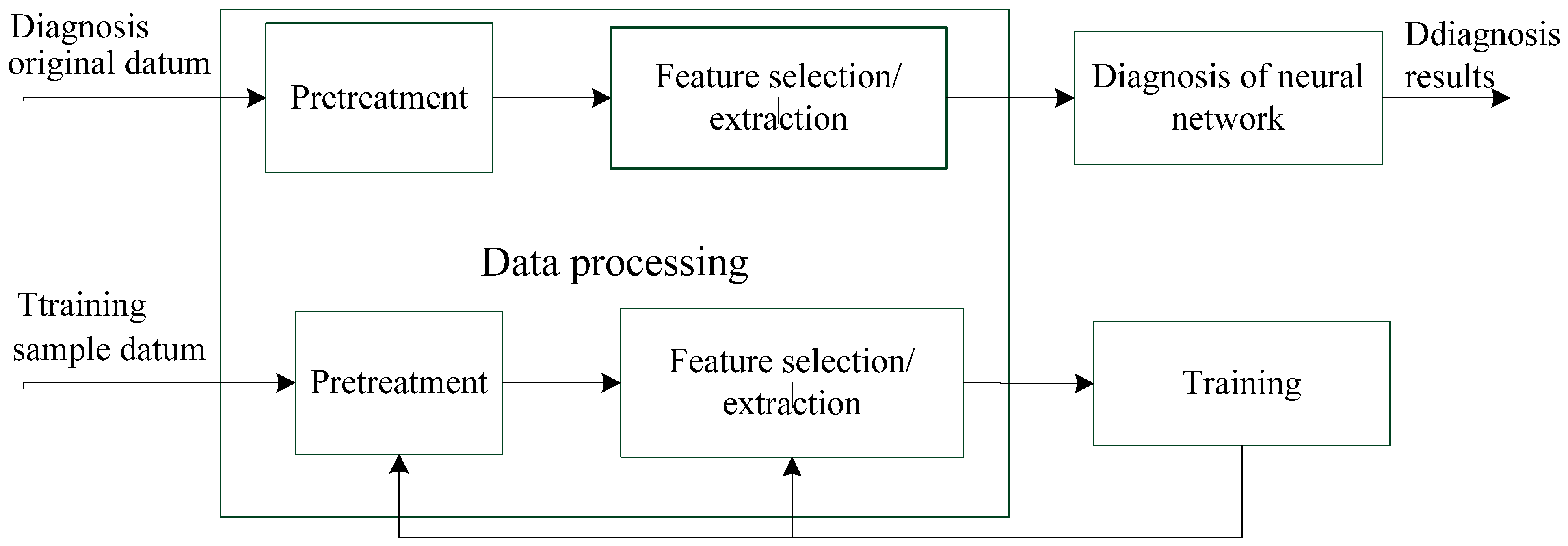
2.2. Structure of Fault Diagnosis System and Information Table

The structure of the proposed polymerization kettle neural network fault diagnosis system is shown in Figure 3. Firstly, a set of fault samples are used to train the neural network to obtain the structure parameters. Then, the pattern classification of faults is made to realize the nonlinear mapping from symptom set to fault set according to a given set of symptoms.

Figure 3. Structure of neural network fault diagnosis system.

Figure 3. Structure of neural network fault diagnosis system.

The proposed fault diagnosis is applied to a certain 70 M3 polymerization kettle from a large chemical company with the measured data. The condition attributes of the decision table are the reducer vibration value of polymerization kettle (mm), the stirring current (A), the pressure of mechanical seal (MPa), the operating pressure (MPa), the stirring speed (r/min), the reducer temperature (°C), the operating temperature of polymerization kettle (°C) and the mechanical seal temperature (°C), whose corresponding variables are denoted as a, b, c, d, e, f, g and h, respectively. The fault of polymerization reactor includes the motor fault, the deceleration machine fault and the machine seal fault. The main mechanical seal failure forms of machine seal faults are the gland-shaft damage and components damage of machine seal. Assume D is the decision attribute in accordance with the direct reasons of the faults, that is to say D = 0 stands for the normal working conditions of the polymerization kettle, D = 1 stands for the motor fault, D = 2 stands for the reducer fault, D = 3 stands for gland-shaft fault of the polymerization machine seal and D = 4 stands for the fault of polymerize component [3].

Large amounts of on-spot data are collected from the PVC polymerization kettle as input samples and testing samples of the neural network fault diagnosis system. The historical working data of polymeric kettle are shown in Table 1.

Table 1. Historical data of polymeric kettle.

Sample(U)	Historical Datum of Polymerizer								Diagnosis Type (D)
	a	b	c	d	e	f	g	h
1	0.38	119.1	1.55	1.45	93.10	42.6	76.13	29.52	4
2	0.44	188.8	1.00	1.51	93.70	78.9	65.44	82.64	3
3	0.39	138.9	1.01	1.78	93.10	92.3	66.83	29.39	1
4	0.38	133.4	0.88	1.34	92.80	59.9	60.32	83.50	0
5	0.40	140.1	1.61	0.86	56.49	41.5	54.21	29.43	0
$⋮$	$⋮$	$⋮$	$⋮$	$⋮$	$⋮$	$⋮$	$⋮$	$⋮$	$⋮$
380	0.38	138.1	1.15	1.35	91.85	78.8	52.39	29.99	0

Table 1. Historical data of polymeric kettle.

Sample(U)	Historical Datum of Polymerizer								Diagnosis Type (D)
	a	b	c	d	e	f	g	h
1	0.38	119.1	1.55	1.45	93.10	42.6	76.13	29.52	4
2	0.44	188.8	1.00	1.51	93.70	78.9	65.44	82.64	3
3	0.39	138.9	1.01	1.78	93.10	92.3	66.83	29.39	1
4	0.38	133.4	0.88	1.34	92.80	59.9	60.32	83.50	0
5	0.40	140.1	1.61	0.86	56.49	41.5	54.21	29.43	0
$⋮$	$⋮$	$⋮$	$⋮$	$⋮$	$⋮$	$⋮$	$⋮$	$⋮$	$⋮$
380	0.38	138.1	1.15	1.35	91.85	78.8	52.39	29.99	0

3. Probabilistic Neural Network

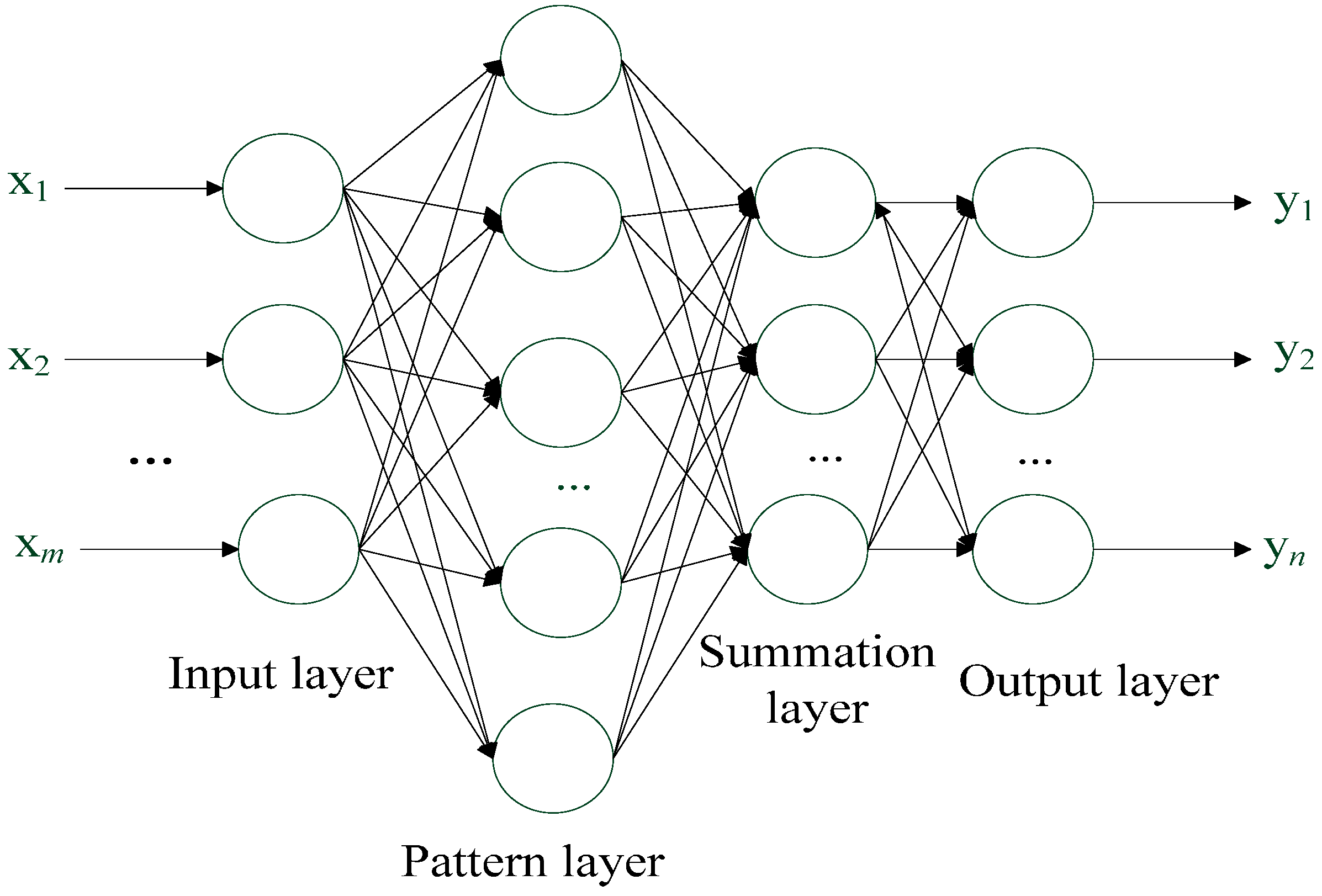
3.1. Structure of PNN

PNN is a kind of self-monitoring feed forward neural network developed from the radial basis function network, whose theory basis is the Bayesian minimum risk criteria (i.e., Bayesian decision theory) [14,15]. In the process of the statistical classification computing, the class conditional probability density can be obtained by Parzen window estimates so as to obtain the classification samples. It does not require training the samples’ connect weights, but directly sets up the hidden layer based on the given training samples. The structure of PNN model is composed of the input layer, the pattern layer, the summation layer and the output layer, whose basic structure is shown in Figure 4.

The input layer receives the training samples data, that is to say the input feature vector of the training samples are fed into the PNN neural network. The number of input layer neurons is equal to the number of characteristics of the training samples parameters. Pattern layer neurons with the same classification number of training samples. The relationship between the input training samples and the various patterns of training samples are calculated. The output of each unit in the pattern layer is calculated by the following equation.

$${\mathrm{\Phi }}_{ij}(x)=\frac{1}{{(2\text{π})}^{d/2}{\text{σ}}^d}\exp \left[-\frac{{(x-x_{ij})}^T(x-x_{ij})}{2{\text{σ}}^2}\right]$$

(1)

where $i=1,\cdots ,M$, $j=1,\cdots ,N$, M is the total number of classes in the training samples, $x_{ij}$ is the jth implicit center vector for the ith mode, $N_i$ is the number of neurons in the pattern layer of the PNN ith calss, σ is the smooth parameter and d is the data dimension of the samples space.

Figure 4. Structure of probabilistic neural network.

Figure 4. Structure of probabilistic neural network.

The summation layer is the cumulative probability belonging to a certain class, which is calculated as follows.

$$f_{i{N}_i}(x)=\frac{1}{N_i}{\displaystyle \sum _{j=1}^{N_i}{\Phi }_{ij}(x)}$$

(2)

Each class is corresponding to units in the summation layer, and units in the summation layer are only connected to the units with their own classes in the pattern layer. Therefore, the input of the summation layer units is only superimposed with its own output in the pattern layer units belonging to its class. The output of the summation layer units is proportional to the probability density estimated values of each class based on the kernel function. By the normalized procession of the output layer units, all kinds of probability estimated values are obtained.

Simple threshold identification constitutes the output decision-making layer of PNN, whose purpose is to select a neuron as the output of the entire system. In the estimated probability density of each fault pattern, this neuron has the largest posterior probability density. Neurons in the output layer are a kind of competitive neuron, in which each neuron is in accordance to a fault pattern with the style of one to one. The number of neurons in the output layer is determined by the training samples, which is the same as the number of fault types of the training samples. All probability density functions in the summation layer are the input of the output layer neurons, which can be described as follows.

$$\text{ρ}(x)=\arg \max [{\text{α}}_i{f}_{i{N}_I}(x)]$$

(3)

where α₁ it the prior probability of the class i and $\text{ρ}(x)$ is the estimated class obtained by PNN.

3.2. Learning Algorithm of PNN

The training steps of PNN based on the input data are described as follows.

Step 1: All the training samples x are expressed in the form of vector $x=(x_1,x_2,\cdots ,x_d)$.

Step 2: The first training sample vector is fed into the neurons of the input layer. Then, the connection weights between the input layer units and the pattern layer units are initialized, that is to say $w_{ 1}=x_1$. So, a connection relationship between the first cell of the pattern layer with the corresponding unit of the accumulate layer is established.

Step 3: For all the rest units, repeat from the first step, that is to say w_m = x_m (m = 1, 2, …, n).

Step 4: In the probabilistic neural network, the input layer and the pattern layers are interconnected with each other after training, and the accumulation layer and the pattern layer is sparsely connected. If the kth component of the jth class samples is denoted as $x_{jk}$, the weight coefficient of $x_{jk}$ to the jth pattern layer unit is referred to as $w_{jk}$ (j = 1, 2, …, n; k = 1, 2, …, d).

Therefore, the classification can be realized according to the following three steps after the trained PNN.

Step 1: A test sample is fed into the input layer. Each unit of the pattern layer is calculated by the followed nonlinear function.

$$f_{\omega }(x)=\frac{1}{{(2\pi )}^{d/2}{\sigma }^d}\exp \left[-\frac{{(x-x_{ij})}^T(x-x_{ij})}{2{\sigma }^2}\right]$$

(4)

Step 2: The calculated results f_ω(x) of the pattern layer neural cells which are connected with the summation layer neural cells is summed. By doing so, a signal is provided for the each summation layer unit connected with the pattern model layer, whose strength is the same as the probability of the test samples. The probability of the test samples is calculated by the Parzen window function with the centers of current training samples.

Step 3: By calculating the results of the summation layer, the desired category of test samples is the maximum calculated result.

4. Rough Set-Probabilistic Neural Network Fault Diagnosis Method Optimized by Shuffled Frog Leaping Algorithm

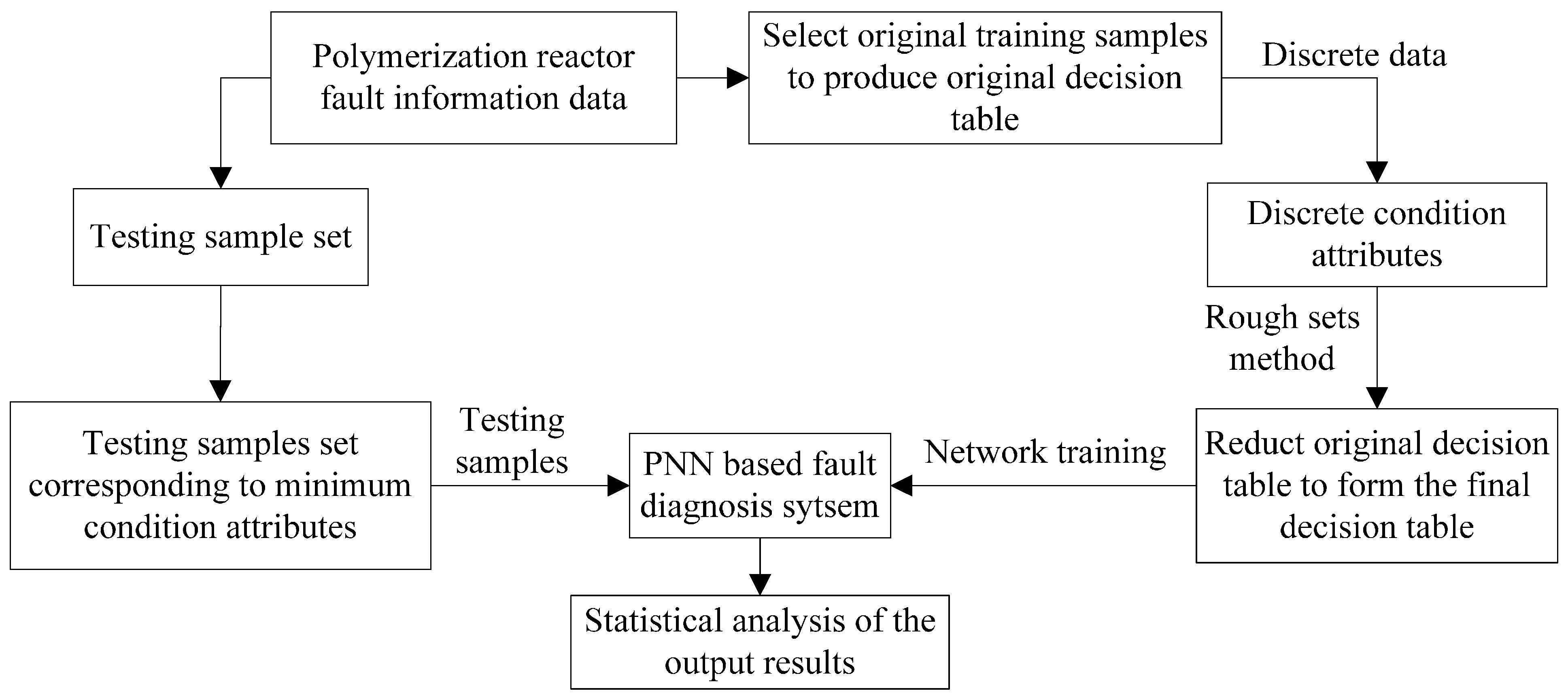
4.1. Polymerization Fault Diagnosis System Based on Rough Set and PNN

The block diagram of the polymerization reactor fault diagnosis system based on rough sets and probabilistic neural network is shown in Figure 5.

The steps of polymerization reactor fault diagnosis by combining both rough sets and probabilistic neural network is described as follows.

Step 1: For the decision table. Collect the process parameters data affecting the running of the polymerization reactor to form the original decision table.

Step 2: Use the RS theory to discrete the original decision table formed by the on-site collected data, and reduce the discrete decision table to form the final decision table.

Step 3: Use the probabilistic neural network to train the final decision table, until the requirements are met. The test samples are selected to realize the fault diagnosis by the trained probabilistic neural network.

Step 4: Carry out the statistical analysis and output the results.

Figure 5. Flowchart of Polymerization fault diagnosis system based on Rough Set and PNN.

Figure 5. Flowchart of Polymerization fault diagnosis system based on Rough Set and PNN.

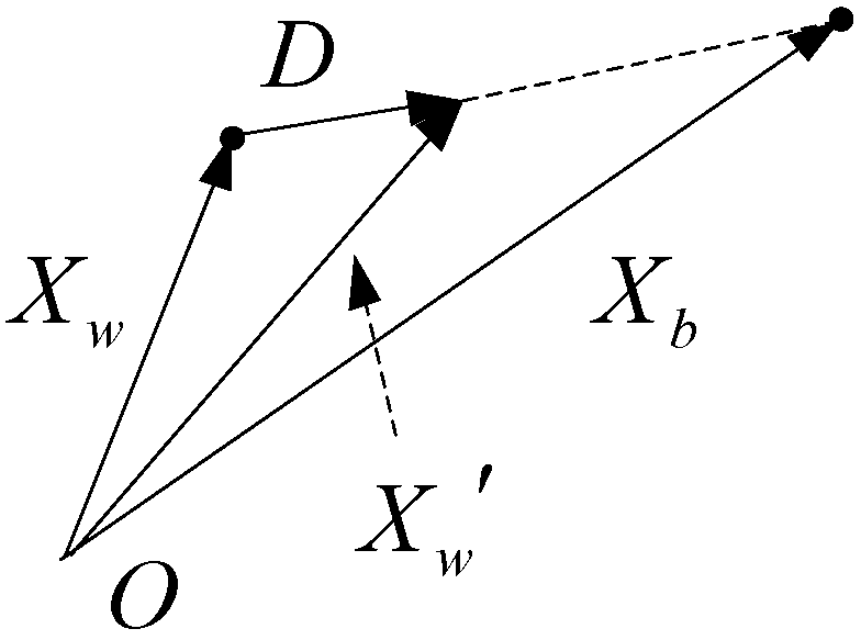
4.2. Attribute Reduction Based on Rough Set (RS) Theory

The rough set (RS) theory proposed by the Polish scientist Z. Pawlak [16,17,18,19] is another new data analysis method applied to the uncertain information mathematical tool in addition to the probability theory and fuzzy set. A large number of historical data from the industrial production process may be ambiguous, uncertain and incomplete. Rough set theory can eliminate redundant information quickly and effectively, dig out the useful knowledge and summarize patterns and rules. Rough set theory deals with the information system through the decision table. Knowledge representation system is also called information system and is described as follows.

$$S=(U,C,D,V,f)$$

(5)

where $U$ is the sample data set, also known as the domain, $C$ is the condition attributes set, $D$ is the decision attributes set, $R=C\cup D$ is the whole attribute set, $V_r$ is the range of attribute values for $r\in R$, $f:U\times R\to V$ is the information function reflecting the attribute values of each individual object in the domain $U$. The knowledge expression system including $C$ and $D$ is defined the decision table, which may be expressed as follows.

$$S=(U,C\cup D,V,f) \text{or} S=(U,R,V,f)$$

(6)

Because the rough set theory can only deal with the discrete attribute values, the data of the fault diagnosis decision-making system have to be assigned discrete values. The results are shown in Table 2.

The attribute reduction method in rough set theory is one of the key research topics. Attribute reduction method based on the discernibility matrix [20] is an important variant of rough set theory, whose main aim is to firstly use the discernibility matrix to derive the discernibility function, and then solve the disjunctive paradigm, where each paradigm is a reduction of the rough set.

Table 2. Fault diagnosis decision table of polymerizer.

Sample (U)	Condition Attribute								Decision Attribute (D)
	S1	S2	S3	S4	S5	S6	S7	S8
1	1	1	2	4	2	2	5	1	4
2	1	2	1	3	2	1	1	1	0
3	1	2	1	3	1	2	1	1	0
4	1	1	2	5	2	4	2	1	1
5	1	2	1	4	2	2	2	2	3
$⋮$	$⋮$	$⋮$	$⋮$	$⋮$	$⋮$	$⋮$	$⋮$	$⋮$	$⋮$
380	1	1	2	4	2	2	5	1	4

Table 2. Fault diagnosis decision table of polymerizer.

Sample (U)	Condition Attribute								Decision Attribute (D)
	S1	S2	S3	S4	S5	S6	S7	S8
1	1	1	2	4	2	2	5	1	4
2	1	2	1	3	2	1	1	1	0
3	1	2	1	3	1	2	1	1	0
4	1	1	2	5	2	4	2	1	1
5	1	2	1	4	2	2	2	2	3
$⋮$	$⋮$	$⋮$	$⋮$	$⋮$	$⋮$	$⋮$	$⋮$	$⋮$	$⋮$
380	1	1	2	4	2	2	5	1	4

Assume S = (U, A, VA, f) is a decision table, $C\cup D=A$, $C\cap D=\Phi$, $\text{D}\ne \Phi$, U = {x₁, x₂, …, x_n}, C is the condition attributes set, D is the decision attributes set and a(x) is a value of the sample attributes. So, the discernibility matrix CD is defined as follows [3]:

$${\text{C}}_{ij}=\{\begin{array}{l}\{\text{a|a}\in {\text{A,a(X}}_i\text{)}\ne {\text{a(X}}_j\text{)}\} D(X_i)\ne D(X_j)\\ 0 D(X_i)=D(X_j)\\ 1 D(X_i)\ne D(X_j),a(X_i)=a(X_j)\end{array}$$

(7)

It can be seen from the definition of a discernibility matrix, $C_{ij}$ is a set composed by all attributes which can distinguish the sample $X_i$ from $X_j$. $\forall X_i$, $X_j\in \text{U}$, $C_{ij}\subseteq A$, which is in accordance with the following properties: (1) $C_{ii}=0$; (2) $C_{ij}=C_{ji}$; (3) $C_{il}\subseteq C_{ij}\cup C_{jl}$.

Attribute reduction method based on the discernibility matrix is adopted to elicit $L=b\wedge c\wedge d\wedge e\wedge g\wedge h$($IND(a,b,c,d,e,f,g,h)=IND(b,c,d,e,g,h)$). That is to say a (the reducer vibration value of polymerization kettle) and f (reducer temperature) are reductive attributes. Then, we delete redundant attributes, combine reduplicate rules and delete the redundant rules in the decision table.

4.3. Shuffled Frog Leaping Algorithm

Shuffled frog leaping algorithm (SFLA) [21] is a kind of sub-acute heuristic coordinated searching swarm algorithm. The SFLA is a meta-heuristic optimization method that mimics the memetic evolution of a group of frogs when looking for the location that has the maximum amount of available food. It is based on evolution of memes carried out by the interactive individuals, and a global exchange of information among themselves. It has been successfully used in water resource network optimization problems [22], assembly line sequencing optimization [23,24,25], flow-shop scheduling problems [26] and clustering problems [27].

The SFLA is described in detail as follows [20]: First, an initial population of N frogs $P=\{X_1,X_2,\cdots ,X_N\}$ is created randomly. For S-dimensional problems (S variables), the position of a frog $i$ in the search space is represented as $X_i=[x_{i1},x_{i2},\cdots ,x_{iS}]$. After the initial population is created, the individuals are sorted in a descending order according to their fitness. Then, the entire population is divided into m memeplexes, each containing n frogs (i.e., $N=m\times n$), in such a way that the first frog belongs to the first memeplex, the second frog goes to the second memeplexe, the mth frog goes to the mth memeplex, and the (m + 1)th frog goes back to the first memeplex, etc. Let $M^k$ is the set of frogs in the kth memeplex, this dividing process can be described by the following expression:

$$M^{ k}=\{X_{k+m(l-1)}\in P|1\le l\le n\},(1\le k\le m)$$

(8)

In the each memeplex, the frogs with the best fitness and worst fitness are identified as $X_b$ and $X_w$. The frog with the global best fitness in the population is identified as $X_g$. Then, the local search is carried out in each memeplex, that is to say the worst frog $X_w$ leaps towards to the best frog $X_b$ according to the original frog leaping rules (shown in the Figure 6) described as follows.

$$D=r\cdot (X_b-X_w)$$

(9)

$${{\mathrm{X}}_{\mathrm{w}}}^{\prime }=X_w+D,(\Vert D\Vert \le D_{\max })$$

(10)

where r is a random number between 0 and 1 and $D_{\max }$ is the maximum allowed change of frog’s position in one jump.

If the new frog ${X_w}^{\prime }$ is better the original frog $X_w$, it replaces the worst frog. Otherwise, $X_b$ is replaced by $X_g$ and the local search is carried out again according to the Equations (9) and (10). If no improvement is made in this case, the worst frog is deleted and a new frog is randomly generated to replace the worst frog $X_w$. The local search continues for a predefined number of memetic evolutionary steps $L_{\max }$ within each memeplex, and then the whole population is mixed together in the shuffling process. The local evolution and global shuffling continue until a convergence iteration number $G_{\max }$ is arrived at.

Figure 6. Schematic chart of frog leaping rule.

Figure 6. Schematic chart of frog leaping rule.

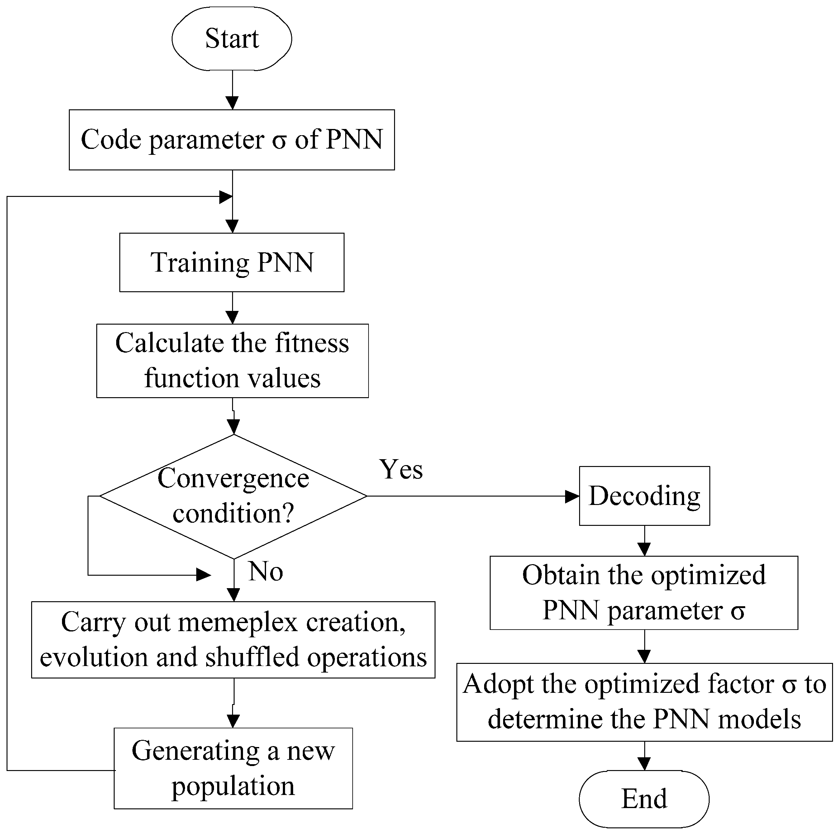
4.4. PNN Optimized by SFLA

SFLA is used to optimize the smoothing factor σ of PNN. However, there is an important issue as to how to reflect the characteristics of the entire sample space σ based on the limited samples. Currently, the most generally used method is the limited sample clustering method or the empirical estimation, but these methods do not meet the probability characteristics to characterize the entire space.

When using SFLA to optimize the parameter in PNN, the smoothing factor set $\stackrel{\prime }{\mathrm{\sigma }}=[{\mathrm{\sigma }}_1,{\mathrm{\sigma }}_2,\cdots ,{\mathrm{\sigma }}_n]$ belonging to the categories N is coded with the float code method. The impact of the Parzen probability estimates values is mainly from its approaching point. When the distance between the test samples and the sample pattern is 2 σ, the corresponding Gaussian function value is 0.136. With the distance 3 σ, the value is 0.011. With the distance 4 σ, the value is 0.0003. So, σ can be obtained by the following equation.

$$\text{σ}=g·d_{av}[k]$$

(11)

where d_av[k] is the average of the minimum distances for the samples in a category and g is a scaling factor (generally from 1.2–2.0).

$$d_{av}[k]=(1/m){\displaystyle \sum _{x_p\in c_k}{d}_i}$$

(12)

where d_i is the minimum distance between class samples and pattern samples. The followed error function is chosen as the fitness function of SFLA.

$$E_P={\displaystyle \sum _{i=1}^P{E}_P}=\frac{1}{2}{\displaystyle \sum _{i=1}^P\Vert d(x_j)-y(x_j)\Vert }$$

(13)

where d(x_j) is the desired output and y(x_j) is the actual output of PNN.

The flowchart of the PNN optimized by SFLA is shown in Figure 7. So, the steps of PNN model optimized by SFLA are described as follows.

Figure 7. Flowchart of PNN optimized by SFLA.

Figure 7. Flowchart of PNN optimized by SFLA.

The algorithmic procedure of the SFLA is described as follows:

Step 1: Initialize the SFLA parameters. Initialize the frog population size N, the search space dimension S, the meme groups number m (each meme group contains n frog (N = m × n), the local search number L_max and the global hybrid iteration number G_max and maximum local search radius r_max.

Step 2: Frog population creation. Calculate the minimum distance average set {dav[k]} between training samples and similar sample space. Randomly initial the population of N frogs $P=\{X_1(t),\cdots ,X_k(t)\cdots ,X_N(t)\} = \{{\text{σ}}_1^{\prime }(t),{\text{σ}}_2^{\prime }(t),\cdots ,{\text{σ}}_N^{\prime }(t)\} (k=1,\cdots ,N)$. Set the iteration counter t = 0. Then, each frog Xk(t) is set as the smoothing factor of the PNN. Each individual’s fitness value $F_k(t)=F(X_k(t))$ is calculated according to Equation (13) after the simulation. Finally, the frogs are sorted in a descending order according to their fitness. The outcome is stored with the style $U_k(t)=\{X_k(t),F_k(t)\}$. The global best frog in the frog population is identified as $X_g(t)=U_1(t)$.

Step 3: Memeplex creation. The U is divided into the m memeplex $M^1(t),\cdots ,M^j(t),\cdots ,M^m(t) (j=1,\cdots ,m)$ according to Equation (8). Each memeplex includes n frogs. The frogs with the best fitness and worst fitness in the memeplex are identified as $X_b^j(t)$ and $X_w^j(t)$.

Step 4: Memeplex evolution. The worst frog $X_w^j(t)$ in the memeplex $M^j(t)$ is carried out the local search based on the frog leaping rule to produce a new frog, that is to say decide the frog leaping step according to Equation (9) and update the position according to Equation (10). Then, the new frog is set as the smoothing factor of the PNN. Its fitness value is calculated after the simulation. If the new frog is better than the original frog, then the $X_w^j(t)$ is substituted. Otherwise, $X_b^j(t)$ is substituted by $X_g(t)$ to carry out the local search again. If no improvement is made, a new frog is created randomly to substitute the . The local search is gone on the L_max iteration to obtain the improved memeplex M¹(t)', M²(t)',⋯, M^m(t)'.

Step 5: The memeplex is shuffled. The frogs in the iterated memeplex M¹(t)', M²(t)',⋯, M^m(t)' are mixed together in the shuffling process and identified as U(t+1) = {M¹(t)¹, M²(t)',⋯, M^m(t)'}. Then, the frogs in the U(t + 1) are sorted in a descending order according to their fitness. The new global best frog in the population is identified as X_g(t + 1) = U₁(t + 1).

Step 6: Test the algorithm termination condition. t = t + 1, if t < G_max, then go to step 3. Otherwise the best frog is determined.

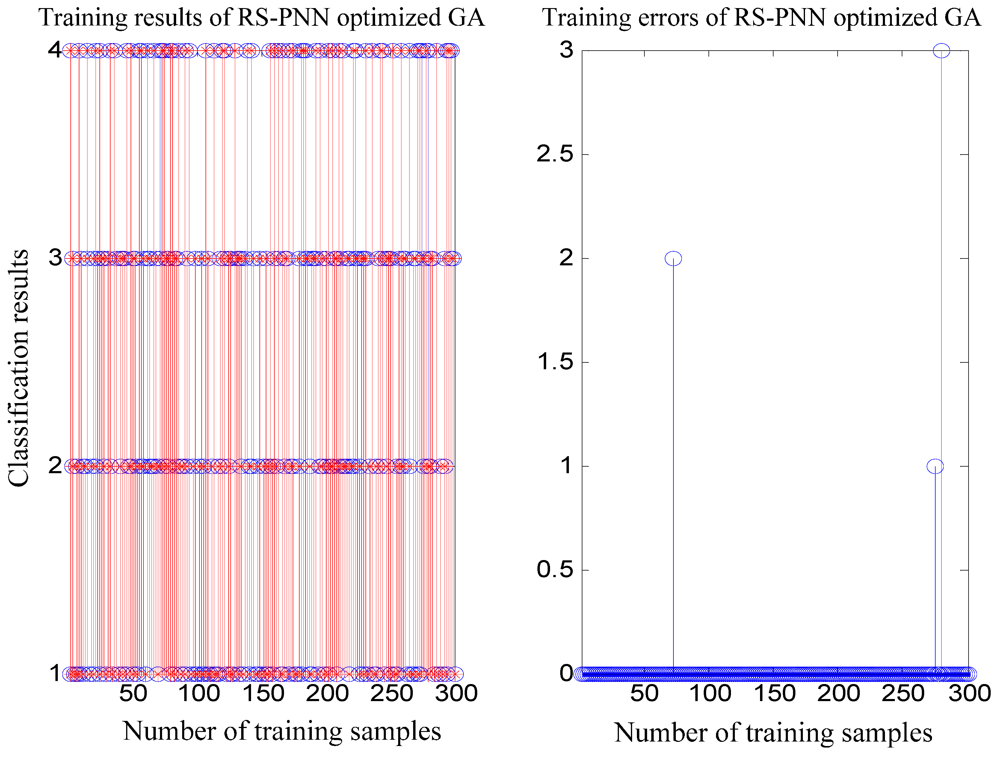
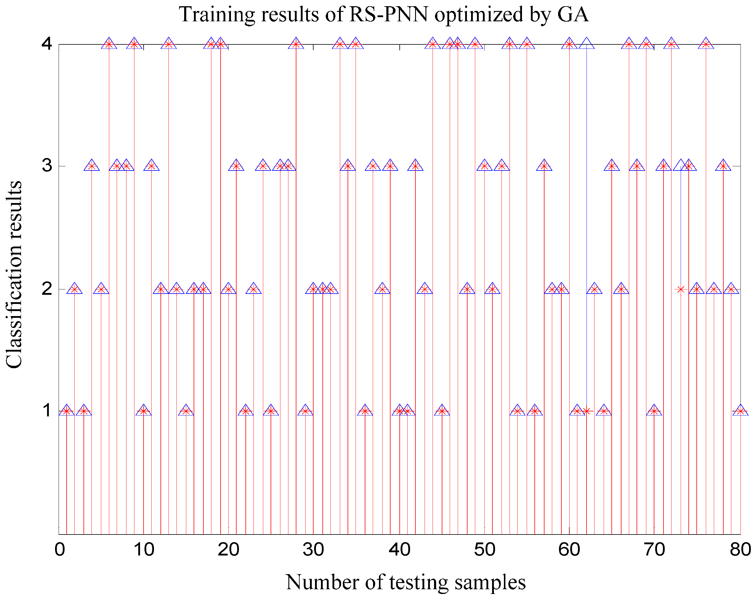
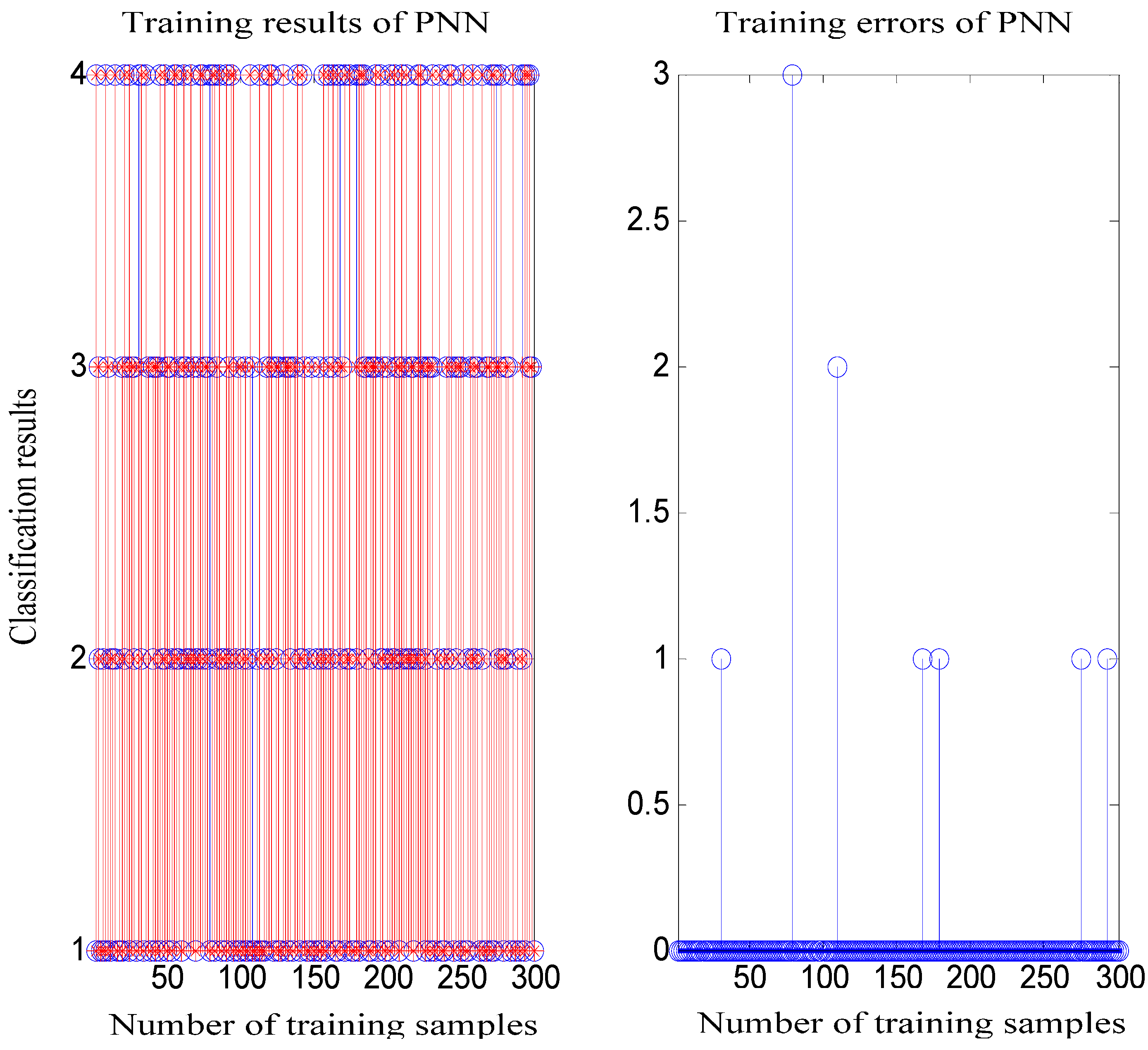
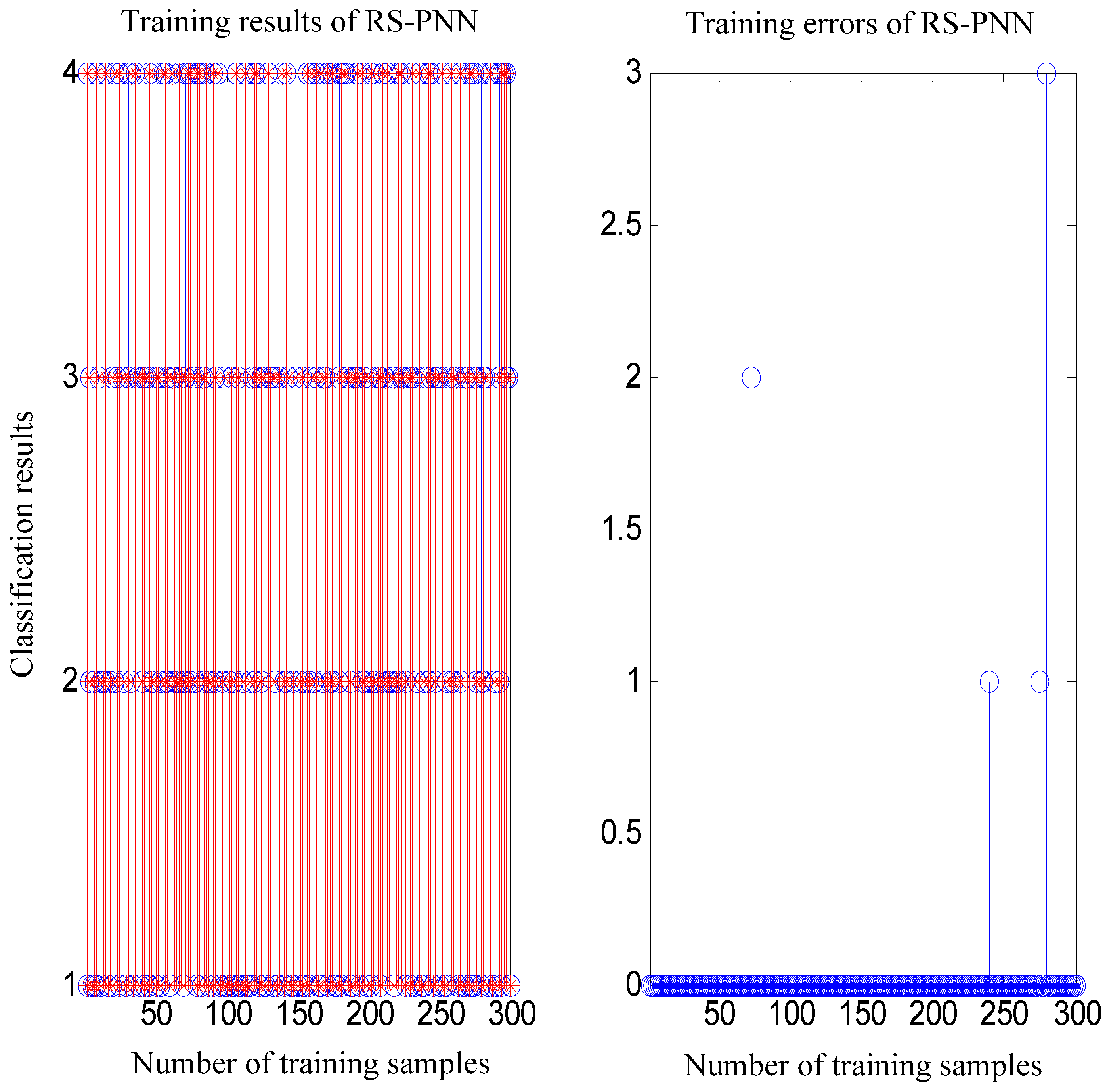
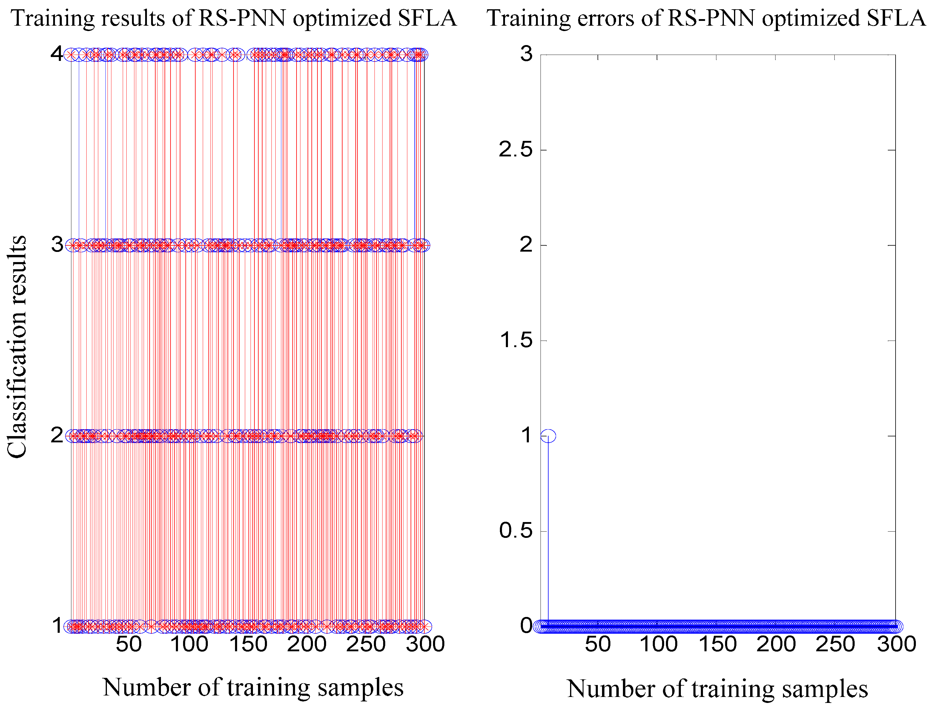
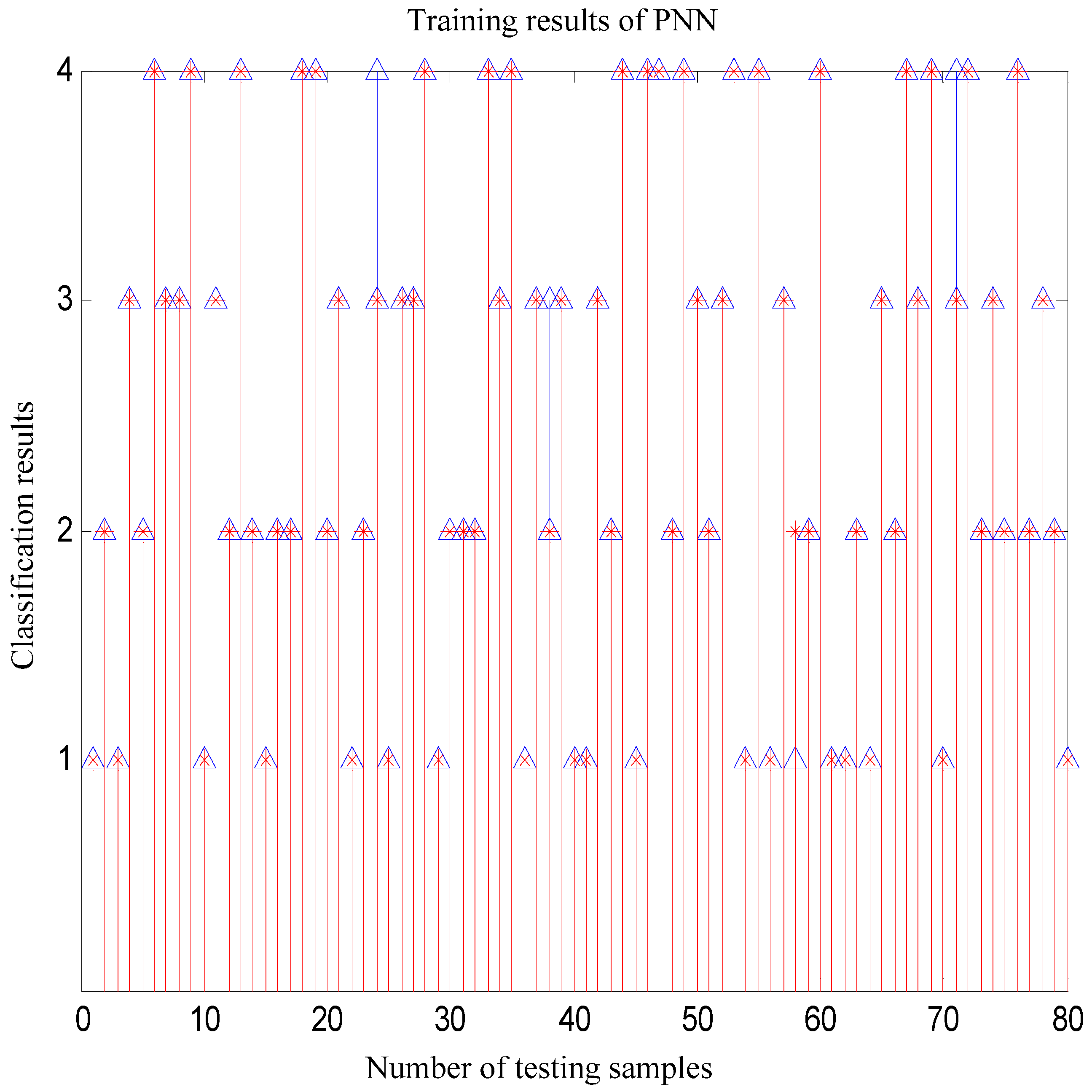
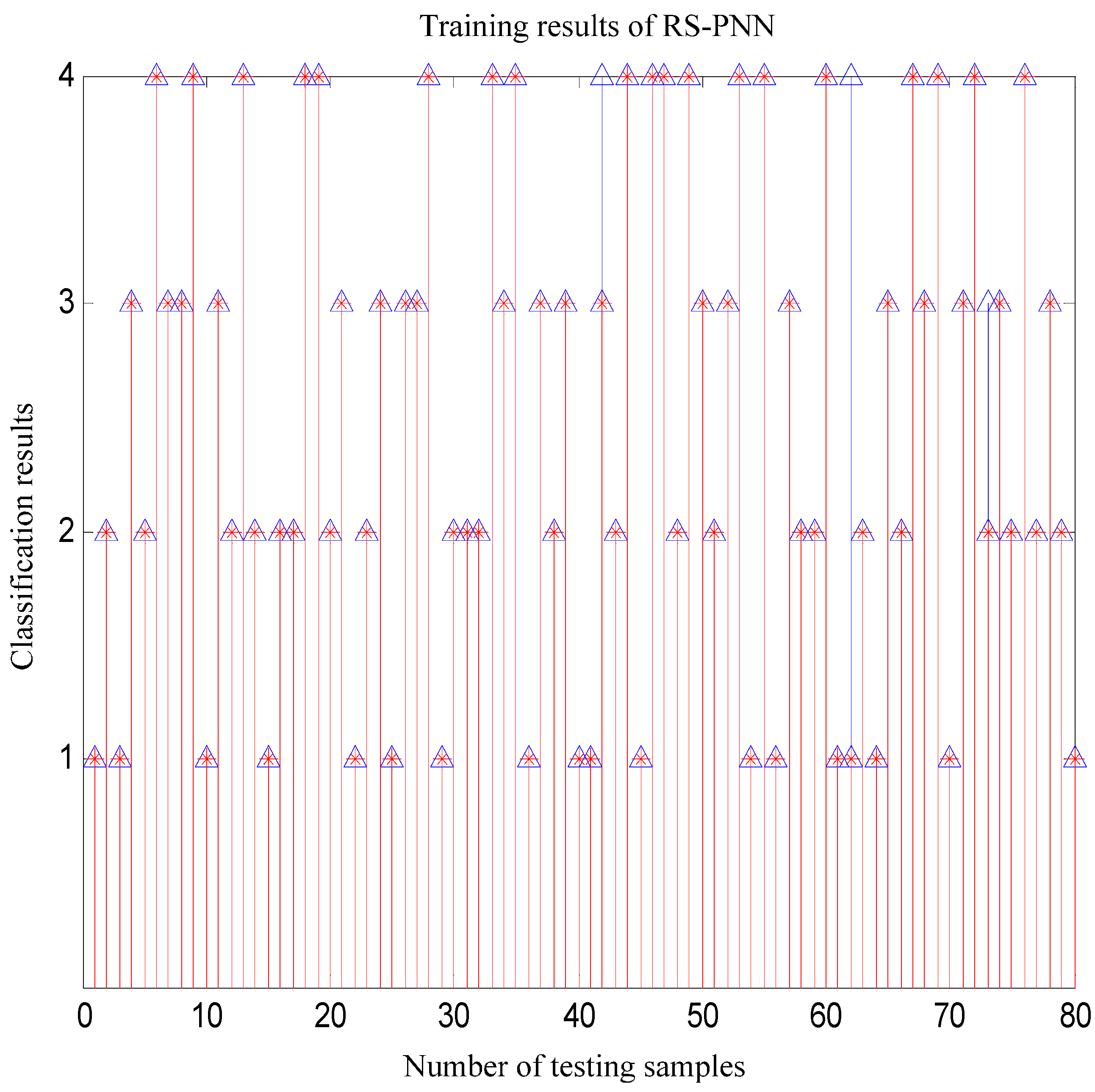
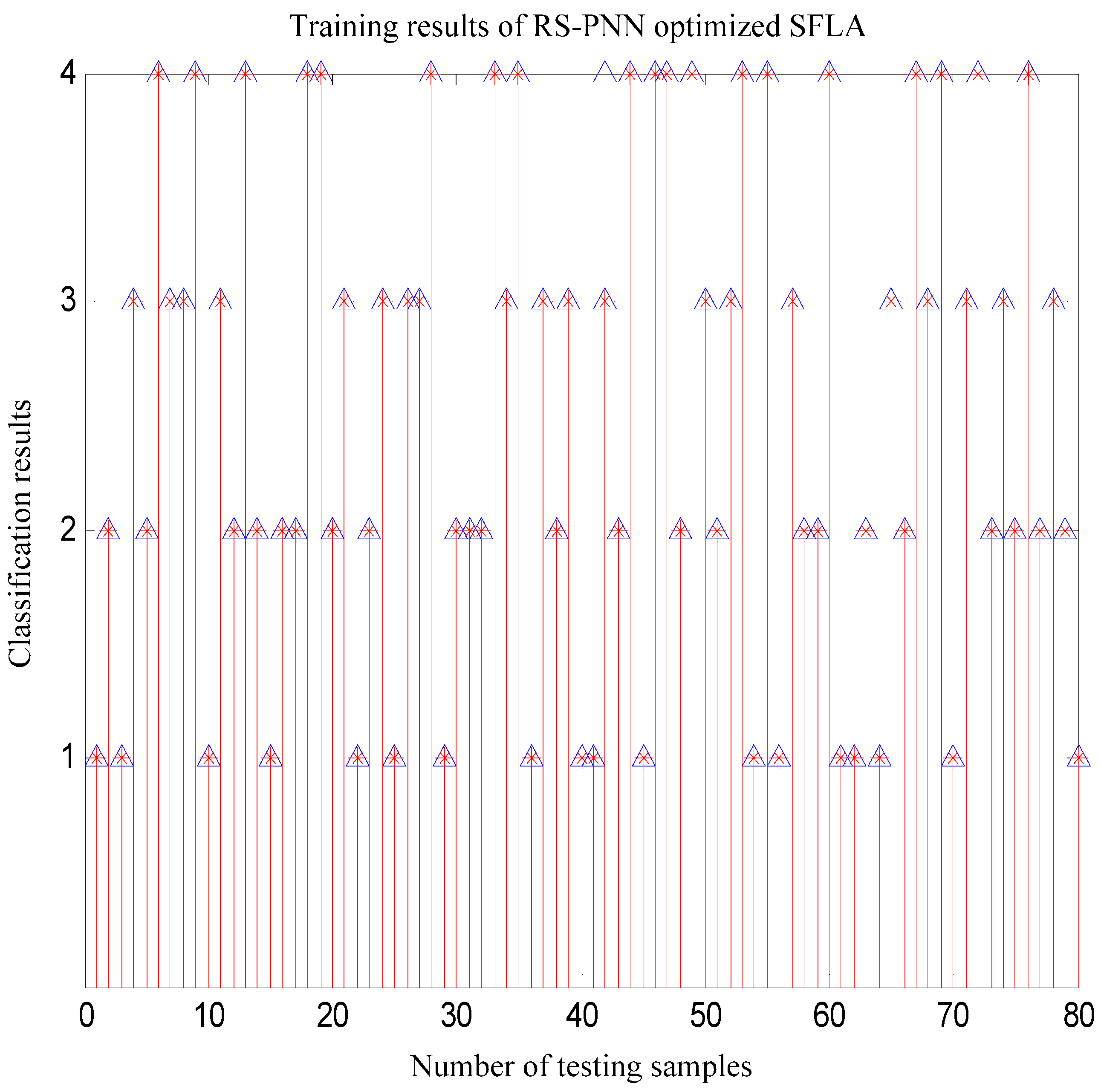
5. Simulation Experiments and Results Analysis

In this paper, the proposed rough set-probabilistic neural network optimized by SFLA is used to realize the fault diagnosis of the polymerization reactor equipment, which is compared with simple PNN, RS-PNN, RS-PNN optimized by genetic algorithm (GA). Firstly, the algorithm parameters are initialized. The parameters of SFLA are described as follows: frog population size N = 50, search space dimensional number S = 1, memetic number m = 5, frog number included in every memetic n = 10, the permitted changeable position maximum value D_max = 0.02, local search iteration number L_max = 5 and the global hybrid iteration number G_max = 100. For genetic algorithm, the number of initial population is 50, the crossover probability is 0.7, the mutation probability is 0.004, the maximum iterations number is 100 and the standard error of the fitness convergence is 0.85. Three hundred sets of data are used as the training samples described in Table 2 and the remaining 80 sets of data as the test data. The simulation results are shown in Figure 8, Figure 9, Figure 10, Figure 11, Figure 12, Figure 13, Figure 14 and Figure 15.

Figure 8. Classification results of PNN under training samples.

Figure 8. Classification results of PNN under training samples.

Figure 9. Classification results of RS-PNN under training samples.

Figure 9. Classification results of RS-PNN under training samples.

In Figure 8, seven training samples have errors after the completed training. In Figure 9, four training samples have errors after the completed training. In Figure 10, three training samples have errors after the completed training. In Figure 11, one training sample has an error after the completed training. By comparing the classification results under four fault diagnosis methods, it can be seen that the training errors significantly reduced though RS-PNN optimized by SFLA. In Figure 12, four training samples have errors after the completed training with testing samples and the diagnostic accuracy was 95%. Similarly, there are three test samples with a diagnosis error in Figure 13 and the diagnostic accuracy is 96.25%. At the same time, there are two test samples with a diagnosis error in Figure 14 and the diagnostic accuracy is 97.50%. There is one test sample with a diagnosis error in Figure 15 and the diagnostic accuracy is 98.75%. The diagnostic accuracy under the RS-PNN optimized by SFLA is the highest among these fault diagnosis methods.

Figure 10. Classification results of RS-PNN optimized by GA under training samples.

Figure 10. Classification results of RS-PNN optimized by GA under training samples.

Figure 11. Classification results of RS-PNN optimized by SFLA under training samples.

Figure 11. Classification results of RS-PNN optimized by SFLA under training samples.

Figure 12. Classification results of PNN under testing samples.

Figure 12. Classification results of PNN under testing samples.

Figure 13. Classification results of RS-PNN under testing samples.

Figure 13. Classification results of RS-PNN under testing samples.

Figure 14. Classification results of RS-PNN optimized by GA under testing samples.

Figure 14. Classification results of RS-PNN optimized by GA under testing samples.

Figure 15. Classification results of RS-PNN optimized by SFLA under testing samples.

Figure 15. Classification results of RS-PNN optimized by SFLA under testing samples.

6. Conclusions

This paper presents a polymerization reactor fault diagnosis strategy based on RS-PNN. The rough set theory is to dispose the input vector of the probabilistic neural network for reducing the dimensionality of the PNN and enhancing its immunity. The shuffled frog leaping algorithm is used to optimize the smoothing factor σ of the PNN. In the end, combining the historical data of the polymerization reactor, the simulation results show the effectiveness of the proposed RS-PNN fault diagnosis strategy.

References

1. Zhou, S.; Ji, G.; Yang, Z.; Chen, W. Hybrid intelligent control scheme of a polymerization kettle for ACR production. Knowl.-Based Syst. 2011, 24, 1037–1047. [Google Scholar] [CrossRef]
2. Gao, S.Z.; Wang, J.S. Design of fault diagnosis system for polymerizer process based on neural network expert system. In Proceedings of the 2011 International Conference on Electric Information and Control Engineering (ICEICE 2011), Wuhan, China, 15–17 April 2011; pp. 3171–3174.
3. Gao, S.Z.; Wang, J.S.; Zhao, N. Fault Diagnosis Method of Polymerization Kettle Equipment Based on Rough Sets and BP Neural Network. Math. Probl. Eng. 2013, 2013, 768018. [Google Scholar]
4. Wang, J.S.; Gao, J. Data driven fault diagnose method of polymerize kettle equipment. In Proceedings of the 2013 32nd Chinese Control Conference (CCC 2013), Xi’an, China, 26–28 July 2013; pp. 7912–7917.
5. Venkatesh, S.; Gopal, S. Orthogonal least square center selection technique—A robust scheme for multiple source Partial Discharge pattern recognition using Radial Basis Probabilistic Neural Network. Expert Syst. Appl. 2011, 38, 8978–8989. [Google Scholar] [CrossRef]
6. Saritha, M.; Joseph, K.P.; Mathew, A.T. Classification of MRI brain images using combined wavelet entropy based spider web plots and probabilistic neural network. Pattern Recognit. Lett. 2013, 34, 2151–2156. [Google Scholar] [CrossRef]
7. Chung, T.Y.; Chen, Y.M.; Tang, S.C. A hybrid system integrating signal analysis and probabilistic neural network for user motion detection in wireless networks. Expert Syst. Appl. 2012, 39, 3392–3403. [Google Scholar] [CrossRef]
8. Timung, S.; Mandal, T.K. Prediction of flow pattern of gas-liquid flow through circular microchannel using probabilistic neural network. Appl. Soft Comput. 2013, 13, 1674–1685. [Google Scholar] [CrossRef]
9. Jiang, S.F.; Fu, C.; Zhang, C. A hybrid data-fusion system using modal data and probabilistic neural network for damage detection. Adv. Eng. Softw. 2011, 42, 368–374. [Google Scholar] [CrossRef]
10. Xu, J.; Liu, C.; Zhou, Q. Study on Steam Turbine Fault Diagnosis of Fish-Swarm Optimized Probabilistic Neural Network Algorithm. In Future Intelligent Information Systems; Springer: Berlin/Heidelberg, Germany, 2011; pp. 65–72. [Google Scholar]
11. Ngaopitakkul, A.; Jettanasen, C. Combination of discrete wavelet transform and probabilistic neural network algorithm for detecting fault location on transmission system. Int. J. Innov. Comput. Inf. Control 2011, 7, 1861–1874. [Google Scholar]
12. Wang, C.; Zhou, J.; Qin, H.; Li, C.; Zhang, Y. Fault diagnosis based on pulse coupled neural network and probability neural network. Expert Syst. Appl. 2011, 38, 14307–14313. [Google Scholar]
13. Er, O.; Tanrikulu, A.C.; Abakay, A.; Temurtas, F. An approach based on probabilistic neural network for diagnosis of Mesothelioma’s disease. Comput. Electr. Eng. 2012, 38, 75–81. [Google Scholar] [CrossRef]
14. Mantzaris, D.; Anastassopoulos, G.; Adamopoulos, A. Genetic algorithm pruning of probabilistic neural networks in medical disease estimation. Neural Netw. 2011, 24, 831–835. [Google Scholar] [CrossRef] [PubMed]
15. Sankari, Z.; Adeli, H. Probabilistic neural networks for diagnosis of Alzheimer’s disease using conventional and wavelet coherence. J. Neurosci. Methods 2011, 197, 165–170. [Google Scholar] [CrossRef] [PubMed]
16. Chatterjee, S.; Bandopadhyay, S. Reliability estimation using a genetic algorithm-based artificial neural network: An application to a load-haul-dump machine. Expert Syst. Appl. 2012, 39, 10943–10951. [Google Scholar] [CrossRef]
17. Yao, Y. The superiority of three-way decisions in probabilistic rough set models. Inf. Sci. 2011, 181, 1080–1096. [Google Scholar] [CrossRef]
18. Qian, Y.; Liang, J.; Pedrycz, W.; Dang, C. An efficient accelerator for attribute reduction from incomplete data in rough set framework. Pattern Recognit. 2011, 44, 1658–1670. [Google Scholar] [CrossRef]
19. Chen, Y.; Miao, D.; Wang, R.; Wu, K. A rough set approach to feature selection based on power set tree. Knowl.-Based Syst. 2011, 24, 275–281. [Google Scholar] [CrossRef]
20. Yao, Y.; Zhao, Y. Discernibility matrix simplification for constructing attribute reducts. Inf. Sci. 2009, 7, 867–882. [Google Scholar] [CrossRef]
21. Huynh, T.-H. A modified shuffled frog leaping algorithm for optimal tuning of multivariable PID controllers. In Proceedings of the 2008 IEEE International Conference on Industrial Technology, Chengdu, China, 21–24 April 2008; pp. 1–6.
22. Eusuff, M.M.; Lansey, K.E. Optimization of water distribution network design using the shuffled frog leaping algorithm. J. Water Resour. Plan. Manag. 2003, 129, 210–225. [Google Scholar] [CrossRef]
23. Elbeltagi, E.; Hezagy, T.; Grierson, D. Comparison among five evolutionary-based optimization algorithms. Adv. Eng. Inform. 2005, 19, 43–53. [Google Scholar] [CrossRef]
24. Rahimi-Vahed, A.; Mirzaei, A.H. A hybrid multi-objective shuffled frog-leaping algorithm for a mixed-model assembly line sequencing problem. Comput. Ind. Eng. 2007, 53, 642–666. [Google Scholar] [CrossRef]
25. Zhu, G.-Y. Meme triangular probability distribution shuffled frog-leaping algorithm. Comput. Integr. Manuf. Syst. 2009, 15, 1979–1985. [Google Scholar]
26. Rahimi-Vahed, A.; Dangchi, M.; Rafiei, H. A novel hybrid multi-objective shuffled frog-leaping algorithm for a bi-criteria permutation flow shop scheduling problem. Int. J. Adv. Manuf. Technol. 2009, 41, 1227–1239. [Google Scholar] [CrossRef]
27. Amiri, B.; Fathian, M.; Maroosi, A. Application of Shuffled frog-leaping algorithm on clustering. Int. J. Adv. Manuf. Technol. 2009, 45, 199–209. [Google Scholar] [CrossRef]