Article

HSE-GNN-CP: Spatiotemporal Teleconnection Modeling and Conformalized Uncertainty Quantification for Global Crop Yield Forecasting

by
Salman Mahmood
1,
Raza Hasan
2,* and
Shakeel Ahmad
2
1
Department of Computer Science, Nazeer Hussain University, ST-2, Near Karimabad, Karachi 75950, Pakistan
2
School of Technology and Maritime Industries, Southampton Solent University, Southampton SO14 0YN, UK
*
Author to whom correspondence should be addressed.
Information 2026, 17(2), 141; https://doi.org/10.3390/info17020141 (registering DOI)
Submission received: 10 December 2025 / Revised: 15 January 2026 / Accepted: 27 January 2026 / Published: 1 February 2026

Abstract

Global food security faces escalating threats from climate variability and resource constraints. Accurate crop yield forecasting is essential; however, existing methods frequently overlook complex spatial dependencies driven by climate teleconnections, such as the ENSO, and lacks rigorous uncertainty quantification. This paper presents HSE-GNN-CP, a novel framework integrating heterogeneous stacked ensembles, graph neural networks (GNNs), and conformal prediction (CP). Domain-specific features are engineered, including growing degree days and climate suitability scores, and explicitly model spatial patterns via rainfall correlation graphs. The ensemble combines random forest and gradient boosting learners with bootstrap aggregation, while GNNs encode inter-regional climate dependencies. Conformalized quantile regression ensures statistically valid prediction intervals. Evaluated on a global dataset spanning 15 countries and six major crops from 1990 to 2023, the framework achieves an R2 of 0.9594 and an RMSE of 4882 hg/ha. Crucially, it delivers calibrated 80% prediction intervals with 80.72% empirical coverage, significantly outperforming uncalibrated baselines at 40.03%. SHAP analysis identifies crop type and rainfall as dominant predictors, while the integrated drought classifier achieves perfect accuracy. These contributions advance agricultural AI by merging robust ensemble learning with explicit teleconnection modeling and trustworthy uncertainty quantification.

Graphical Abstract

1. Introduction

The Food and Agriculture Organization (FAO) estimates that agricultural production must increase by 70% by 2050 to feed a projected population of 9.7 billion [1,2]. To meet this demand, crop yield forecasting has become a critical tool for proactive agricultural planning, allowing stakeholders to anticipate production shortfalls, optimize resource allocation, and design climate adaptation strategies.
Traditional yield prediction relied on historical averages and simple regression. However, the complexity of modern agricultural systems, characterized by nonlinear climate–soil–crop interactions, demands sophisticated data-driven approaches capable of capturing multi-scale spatiotemporal dependencies. Climate teleconnections, particularly the El Niño–Southern Oscillation (ENSO) and North Atlantic Oscillation (NAO), exert profound influence on global weather patterns [3,4]. While these phases modulate precipitation and temperature across key agricultural regions [5,6], teleconnection indices remain inadequately integrated into operational forecasting. These indices are frequently treated as independent scalar features rather than structured spatial dependencies that drive inter-regional climate coupling.
Despite recent advances, contemporary crop yield prediction faces four fundamental limitations:
  • Most machine learning approaches model locations independently or use simplistic spatial features like latitude and longitude. This fails to capture the complex inter-regional coupling induced by teleconnections. Graph neural networks (GNNs) offer a framework for encoding these structured relationships, but their application to agriculture remains nascent [7].
  • Ensemble and Bayesian methods provide uncertainty estimates but often lack finite-sample validity guarantees. Conformal prediction, a distribution-free framework that guarantees marginal coverage under minimal assumptions [8], has seen limited adoption in agricultural AI despite its utility for high-stakes decision-making.
  • The “black-box” nature of deep learning models often impedes stakeholder trust. While model-agnostic explainability methods like SHAP (SHapley Additive exPlanations) can unveil feature importance and interaction effects [9,10], they are underemployed in the current forecasting literature.
  • Yield forecasts are most actionable when accompanied by complementary drought severity classification and calibrated uncertainty bounds. Integrated multi-task frameworks that jointly address prediction, classification, and risk are currently scarce.
To address these gaps, the HSE-GNN-CP framework is introduced, a comprehensive framework with the following contributions:
  • Primary Methodological Contribution: The primary novelty is the development and validation of a conformalized quantile regression (CQR) wrapper for bootstrap ensembles in agricultural forecasting. While bootstrap methods are common for generating prediction distributions [11], they frequently suffer from significant under-coverage in yield data. The CQR approach provides a rigorous finite sample coverage guarantee in this domain [8], correcting uncalibrated bootstrap intervals from 40.03% to a valid 80.72% coverage. This represents a fundamental shift from heuristic uncertainty estimation to mathematically guaranteed reliability for agricultural risk management.
  • Secondary Innovations and Methodological Integration: In addition to the primary uncertainty framework, three secondary contributions are provided through the novel integration of existing methodologies:
    Global climate structures are explicitly modeled by constructing a spatial graph where edges are defined by historical rainfall correlations. A 2-layer graph convolutional network (GCN) is integrated to learn 64-dimensional embeddings that propagate information along these teleconnection pathways [7,11,12], This provides a structured representation of climate dependencies that improves predictive accuracy over standard spatial features.
    The machine learning pipeline integrates biophysical constraints through engineered features such as growing degree days (GDD), moisture stress index (MSI), and climate suitability score (CSS) [8,13,14]. SHAP analysis explains model behavior and confirms alignment with established plant physiology.
    The synergistic benefit is demonstrated a holistic framework that jointly performs yield prediction and drought severity classification via MSI thresholds. Testing this integrated pipeline on a global multi-crop dataset produces a comprehensive decision support tool that outperforms fragmented single task models.

2. Related Work

The development of robust crop yield forecasting systems sits at the intersection of agronomy, climate science, and advanced machine learning. To contextualize the contributions of the HSE-GNN-CP framework, it is necessary to examine existing methodologies across four distinct but interconnected domains: the evolution of predictive modeling architectures, the integration of global climate teleconnections, the rigor of uncertainty quantification techniques, and the interpretability of complex AI systems. The following subsections critically review recent advancements and identify persistent gaps in each of these areas.

2.1. Crop Yield Prediction

Crop yield prediction is made increasingly accurate and sophisticated through advanced machine learning techniques that integrate environmental and agricultural data. Multiple studies demonstrate the power of predictive models, with accuracy ranging from 63% to 99% [15]. Researchers have developed complex models using random forest, neural networks, and support vector machines that analyze critical factors like temperature, humidity, rainfall, and soil conditions [16,17]. Key breakthroughs in the field include integrating remote sensing data [18], utilizing comprehensive datasets spanning multiple years, and achieving prediction accuracies up to 94% with stacked models [15]. These advances promise significant benefits for agricultural planning and food security, providing a strong foundation for the heterogeneous ensemble approach proposed in this work.

2.2. Climate Teleconnections in Agriculture

Climate teleconnections are critical mechanisms that significantly influence global agricultural productivity through complex ocean–atmospheric interactions. Ref. [19] found that climate oscillations correlate with crop yield variability across half of maize and wheat harvested areas, with the El Niño–Southern Oscillation (ENSO) being particularly impactful. Ref. [20] emphasize that seasonal weather fluctuations strongly influence crop yields, with teleconnections contributing to extreme weather events. The evidence suggests robust global patterns: the ENSO affects crop production on all continents [19], while other oscillations like the North Atlantic Oscillation (NAO) and Indian Ocean Dipole (IOD) have region-specific impacts [21]. Critically, these teleconnections can potentially be forecasted in advance, offering opportunities to improve agricultural resilience to climate-related shocks.
Climate teleconnections have been extensively studied in agricultural contexts beyond the initial work. Ref. [22] quantified the ENSO’s asymmetric impacts during El Niño versus La Niña phases on South American soybean production, finding yield losses of 15–20% during strong El Niño events but only 5–10% gains during La Niña. Ref. [23] demonstrated that the NAO’s influence on European wheat yields varies by season, with stronger effects during the booting stage when temperature sensitivity peaks. Ref. [24] developed teleconnection-based seasonal forecasting models for rice in Southeast Asia, achieving 3–6-month lead times by incorporating the IOD (Indian Ocean Dipole) alongside the ENSO.
Recent advances in GNN-based agricultural forecasting include [25,26,27,28], who applied graph attention networks to model spatial dependencies in county-level US corn yields, achieving 5% RMSE reduction compared to spatial regression baselines. Ref. [29] used spatio-temporal GCNs for wheat yield forecasting across European regions, demonstrating that graph structure based on climatic similarity outperforms geographic proximity alone. However, these works did not explicitly encode teleconnection patterns. The contribution lies in constructing graphs from rainfall correlations aligned with known ENSO/NAO pathways, validated through ablation studies demonstrating measurable improvements.

2.3. Uncertainty Quantification

Uncertainty quantification (UQ) is a critical process in agricultural modeling that systematically identifies, measures, and manages the inherent variabilities and unknowns in agricultural systems and predictions. Ref. [30] found that crop model processes are the primary source of uncertainty, accounting for over 50% of variability in agricultural projections. Ref. [31] demonstrated that uncertainties stem from multiple sources, including initial conditions, soil inputs, meteorological forcing, management practices, and model parameters. Researchers have developed sophisticated approaches to address these complexities, such as the hybrid statistical–physical framework proposed by [32] and the cross-sectoral approaches emphasized by [33]. The ultimate goal is to provide more robust decision-making tools for agricultural planning and climate adaptation.
To achieve this in computational forecasting, various statistical methods have been explored. Efron’s bootstrap generates prediction distributions by resampling training data and aggregating model outputs, a computationally simple approach that often exhibits under-coverage due to distributional mis-specification. Alternatively, Bayesian neural networks and Gaussian processes propagate uncertainty via posterior distributions, yet they require careful prior specification and incur computational overhead that scales poorly with data size [34,35]. To address these limitations, conformal prediction was introduced as a distribution-free framework providing finite-sample valid prediction intervals under the exchangeability assumption [36].
Recent applications from 2022 to 2024 demonstrate growing adoption of conformalized methods for agricultural uncertainty quantification [37,38]. Ref. [39] applied split conformal prediction to county-level maize yield intervals in the US Corn Belt, achieving valid 90% coverage while maintaining narrower intervals than bootstrap percentile methods. Ref. [40] proposed adaptive conformal prediction for time-series crop forecasting, adjusting coverage guarantees under non-stationarity induced by climate change. Furthermore, Ref. [41] demonstrated conformal prediction for multi-horizon wheat yield forecasts in Australia, showing that finite-sample guarantees hold even for ensemble predictions.
This work extends these applications by combining conformalized quantile regression (CQR) with heterogeneous bootstrap ensembles. This approach addresses both conditional and marginal coverage while maintaining computational efficiency suitable for operational forecasting systems [42].

2.4. Explainability in Agricultural AI

Explainable AI (XAI) is transforming agricultural decision-making by providing transparent, interpretable insights into complex AI models, addressing the critical “black box” problem in agricultural technology. Multiple studies demonstrate XAI’s potential across agricultural domains [43]. Ref. [44] highlights XAI’s role in enhancing precision agriculture through techniques like LIME, SHAP, and Grad-CAM, enabling informed decisions in crop management, yield prediction, and resource optimization. Thakur et al. emphasize that XAI helps farmers trust AI recommendations by explaining how decisions are made. Key applications include crop recommendation [45], predictive maintenance [46], and livestock monitoring [47]. While promising, challenges remain in model complexity, data quality, and farmer technological literacy. The research unanimously suggests XAI is crucial for democratizing AI in agriculture and supporting sustainable farming practices.
Explainability in agricultural AI operates at two complementary levels, both of which are essential for stakeholder trust and actionable insights [48]. Global explainability methods, such as feature importance rankings and aggregated SHAP values, reveal general patterns across entire datasets [43]. These techniques identify which variables most influence crop yields overall and how climate factors, such as temperature, typically affect predictions [49,50] Global explanations support policy-level decisions, model validation against established agronomic theory, and the identification of universal relationships [51].
Conversely, local explainability techniques explain specific predictions for particular fields, regions, or years [48]. These methods address why a model predicted a specific yield shortfall for an individual farm in each season or which factors drove an anomalous forecast for a specific region [52]. Local explanations enable farmer-level decision support, auditing of model behavior on outliers, and the validation of specific recommendations against local expert knowledge [53].
Recent agricultural XAI applications highlight this growing diversity. Ref. [54] used LIME for explainable pest detection in computer vision models, while Ref. [55] applied attention mechanisms for disease classification with visual explanations. Additionally, Ref. [56] demonstrated the use of SHAP for soil moisture prediction interpretability.
This work employs TreeSHAP [57] because it provides a unified framework for both global and local perspectives. Grounded in coalitional game theory, SHAP provides additive feature attributions that are more consistent and theoretically sound than standard tree-based metrics. Global SHAP rankings validate alignment with agronomic priorities. Local explanations provide instance level transparency for operational forecasting systems.

3. Problem Formulation and Dataset

This section formalizes the computational framework for the HSE GNN CP system and describes the data infrastructure supporting the experiments. Developing a robust agricultural decision-support tool requires a clear mathematical definition of the predictive tasks, specifically point forecasting, uncertainty quantification, and drought risk classification. Furthermore, capturing the complex drivers of crop yield necessitates a comprehensive dataset that integrates agronomic records with global climate variables and teleconnection indices. The following describes the notation, learning objectives, and the multi-source data compilation process.

3.1. Problem Formulation

Let D = { ( x i , y i ) } i = 1 N be a dataset of N crop yield observations. Each feature vector satisfies x i R d , and each yield value satisfies y i R + . The yield is measured in hectogram per hectare. Each observation i has metadata t i   ( year ) , a i   ( country ) , c i   ( crop   type ) .
The research objectives are defined as follows.
  • Point prediction: Learn a function f : R d R + that produces a yield estimate y ^ = f ( x ) .
  • Uncertainty quantification: Construct prediction intervals [ C ^ l o w e r , C ^ u p p e r ] that satisfy P ( y [ C ^ l o w e r , C ^ u p p e r ] ) 1 α , for a chosen miscoverage rate α , with guarantees under exchangeability.
  • Drought classification: Assign each sample to one of the categories { No   Drought ,   Mild ,   Moderate ,   Severe } using thresholds derived from the moisture stress index.

3.2. Global Crop Yield Dataset

A comprehensive global agricultural dataset was compiled by integrating historical crop yield records, meteorological observations, and climate teleconnection indices.

3.2.1. Data Sources

  • Annual country-level yield data (1990–2023) obtained from the FAO Statistics Division (FAOSTAT) [58].
  • Averaged temperature (°C) and aggregate rainfall (mm/year) derived from global reanalysis products [59].
  • Fertilizer and pesticide consumption data (tonnes per country per year) sourced from the FAO [58].
  • The ENSO index (specifically the Oceanic Niño Index, ONI) from the NOAA Physical Sciences Laboratory, and the NAO index from the Climate Research Unit (CRU) [60].
  • The final processed dataset, including all engineered features and teleconnection indices, has been archived for reproducibility and is available at: https://data.mendeley.com/datasets/y7hkz2zfcc/1 (accessed on 5 December 2025).

3.2.2. Dataset Scope

  • Fifteen countries across six continents: Australia, Brazil, China, Egypt, India, Indonesia, Iran, Kenya, Mexico, Peru, Russia, Thailand, Turkey, USA, Vietnam. These nations represent diverse agro-climatic zones (tropical, temperate, arid, monsoon-influenced) and account for significant global production shares.
  • Six major staples and cash crops: wheat, rice, maize, soybeans, barley, potatoes. Together, these crops dominate global caloric supply and trade volumes.
  • A time span of 34 years (1990–2023), encompassing multiple ENSO cycles, technological adoption phases (e.g., improved seed varieties, precision agriculture), and climate variability trends.
  • N = 3060 observations (15 countries × 6 crops × 34 years = 3060 country–crop–year tuples).

3.3. Feature Space and Descriptive Statistics

Raw features with dimensionality draw = 11.
  • Year t
  • Area or country a, categorical
  • Item or crop c, categorical
  • Latitude in degrees north
  • Longitude in degrees east
  • Average temperature in degrees Celsius
  • Average rainfall in millimeters per year
  • Pesticides in tonnes
  • ENSO index, dimensionless
  • NAO index, dimensionless
  • Yield in hectogram per hectare, target variable
Descriptive statistics:
  • Yield: Mean 37,720 hg per ha. Standard deviation 24,527 hg per ha. Minimum 552 hg per ha. Maximum 151,349 hg per ha. The range reflects differences across crops.
  • Temperature: Mean 17.2 °C. Standard deviation 6.2 °C.
  • Rainfall: Mean 1147 mm per year. Standard deviation 512 mm per year.
  • ENSO index: Mean near 0. Standard deviation 0.58.
  • NAO index: Mean near 0. Standard deviation 0.69.

4. Methodology

This section presents the methodological framework of HSE-GNN-CP, a system for robust global crop yield forecasting. The architecture addresses non-linear climate–crop interactions, spatial interconnectedness driven by teleconnections, and the need for rigorous risk assessment. The framework includes the system architecture, domain-specific feature engineering translating raw climate data into agronomic predictors, a heterogeneous stacked ensemble with conformal calibration for valid uncertainty bounds, a graph neural network for spatial teleconnections, and modules for decision support and explainability.

4.1. System Architecture Overview

HSE-GNN-CP is a modular framework designed to address the challenges of global crop yield forecasting, including non-linear climate interactions, spatial dependencies, and the need for rigorous risk quantification. As illustrated in Figure 1, the system pipeline operates as follows.
The proposed framework operates as an end-to-end pipeline consisting of four interconnected modules: (1) Data Ingestion, where multi-source agricultural and climate data are aggregated; (2) Feature Engineering, which transforms raw inputs into biophysical indicators (GDD, MSI, CSS) and constructs the rainfall correlation graph; (3) the Modeling Framework, featuring a dual-stream approach that processes spatial teleconnection dependencies via graph neural networks (Stream A) while simultaneously generating yield prediction distributions through the HSE-BQU ensemble (Stream B); and (4) Decision Support, which applies CQR to calibrate uncertainty intervals, alongside drought risk classification and SHAP-based explainability analysis.

4.2. Agronomic Feature Construction

Raw agricultural data benefits substantially from domain-informed feature transformations that encode biophysical principles. Four agronomic features are engineered grounded in crop physiology and climate-yield relationships.

4.2.1. Growing Degree Days (GDD)

GDD quantifies heat accumulation required for crop development. Temperature below a crop-specific base threshold Tbase contributes negligibly to growth, while temperatures above Tbase drive phenological advancement as shown in Equation (1) [61].
GDD = m a x ( 0 , T T base ( c ) ) × L
where T is average temperature, Tbase(c) is the base temperature for crop c (e.g., 5 °C for wheat, 10 °C for maize), and L = 150 is a scaling factor representing growing season length (days). Common Tbase values: wheat 5 °C, rice 10 °C, maize/soybeans 10 °C, barley 5 °C, potatoes 7 °C. The scaling factor L = 150 approximates a typical growing season length for annual crops, which is approximately 5 months or 150 days. Sensitivity analysis, detailed in Supplementary Table S1, demonstrates remarkable robustness to this parameter across the range L [ 100 , 200 ] . Specifically, the model maintains identical performance, with an R 2 of 0.9599 and an RMSE of 4948 hg/ha, for all tested values. This complete insensitivity suggests that temperature and other engineered features, such as MSI and CSS, effectively compensate for variations in GDD calculation, eliminating the need for crop-specific or region-specific parameter tuning. The model robustness enhances practical applicability because it does not require precise growing season estimation for different crops or climates.

4.2.2. Moisture Stress Index (MSI)

MSI captures relative water deficit or surplus compared to crop-optimal rainfall Popt(c), as shown in Equation (2) [62].
MSI = P P opt ( c ) P opt ( c )
where P is observed rainfall and Popt(c) is optimal rainfall for crop c (e.g., wheat 500 mm, rice 1500 mm, maize 800 mm, soybeans 700 mm). MSI > 0 indicates excess moisture; MSI < 0 indicates drought. Severe negative MSI correlates with yield penalties.

4.2.3. Climate Suitability Score (CSS)

CSS integrates temperature and rainfall fitness into a single metric as shown in Equation (3).
C S S = exp ( ( T T opt ( c ) ) 2 50 ) Temperature   fitness × ( 1 m i n ( P P opt ( c ) 2 P opt ( c ) , 0.9 ) ) Rainfall   fitness
The temperature variance parameter σ2 = 50 produces a Gaussian kernel with approximately 14 °C half-width (±2σ ≈ ±28 °C), capturing the gradual decline in crop suitability outside optimal temperature ranges while maintaining biological realism. The rainfall penalty cap of 0.9 balances two objectives: preventing negative CSS values (maintaining mathematical interpretability) while allowing strong penalties for extreme rainfall deviation (preserving sensitivity to drought and flood conditions).
Sensitivity analysis (Supplementary Table S2, Supplementary Figure S2) tested 20 parameter combinations (variance ∈ [30, 40, 50, 60, 70], cap ∈ [0.7, 0.8, 0.9, 1.0]), revealing good robustness with **R2 varying by only ±0.0025 (0.26% relative variation) across all configurations. While optimal performance occurs at variance = 40, cap = 1.0 (R2 = 0.9629), the default values (variance = 50, cap = 0.9) achieve near-optimal results (R2 = 0.9599), with a performance gap of only ΔR2 = 0.003 (0.31%). This validates that CSS is not overly sensitive to precise parameter specification and generalizes well across diverse crops and climates without requiring extensive tuning.

4.2.4. Temperature Component

Gaussian kernel centered at Topt(c) (e.g., 20 °C for wheat, 25 °C for rice), with variance parameter 50.

4.2.5. Rainfall Component

Linear penalty for deviation from Popt, capped at 0.9 to prevent negative values. CSS ∈ [0, 1], with values near 1 indicating ideal conditions.

4.2.6. Technology Index

Agricultural productivity increases with technological adoption, including improved varieties, mechanization, and more efficient fertilizer use. This trend is represented using Equation (4).
Tech = ( t 1990 ) × 0.5
where t is the year. This linear trend assumes modest annual gains (0.5 units per year).

4.2.7. Feature Vector Construction

Area (country) and Item (crop type) are categorical variables. Label encoding is applied, mapping each category to an integer index (e.g., Australia → 0, Brazil → 1, …, Vietnam → 14; barley → 0, maize → 1, …, wheat → 5). This preserves cardinality while enabling tree-based models to induce splits. Final Feature Vector (d = 12) is represented by Equation (5).
x = [ t , P , p , T , e , n , GDD , MSI , CSS , Tech , a e n c , c e n c ] T
where p = pesticides, e = ENSO, n = NAO, aenc = encoded area, cenc = encoded crop.

4.3. HSE-BQU: Heterogeneous Stacked Ensemble

To balance the bias–variance trade-off and enable robust uncertainty estimation, the heterogeneous stacked ensemble with bootstrap uncertainty (HSE-BQU) is proposed. HSE-BQU employs a two-level stacking architecture.
  • Level 1 (Base Learners): Two complementary models capture different aspects of the data:
    Random forest (RF): Bagging-based ensemble of decision trees, robust to outliers and capable of modeling complex interactions. Configuration: 50 trees, max_depth = 12, feature subsampling at each split.
    Gradient boosting (GB): Sequential additive model minimizing residuals, effective for capturing fine-grained patterns. Configuration: 50 estimators, max_depth = 5–6, learning rate tuned via validation.
    While both random forest and gradient boosting are tree-based methods, they capture complementary aspects of the data-generating process, which justifies their combined use in the ensemble.
    The random forest bagging approach builds independent trees via bootstrap aggregation. This provides robustness to outliers, stable variance estimates critical for uncertainty quantification, and a parallel ensemble structure that efficiently handles high-dimensional feature spaces. Random forest excels at capturing diverse patterns through randomized feature selection at each split.
    In contrast, the gradient boosting approach sequentially fits trees to residuals. This method excels at capturing fine-grained patterns, complex feature interactions, and subtle relationships missed by parallel ensembles. The additive structure of gradient boosting provides a modeling capacity that is complementary to the averaging approach used in random forest.
    Empirical evaluation confirms these distinct error profiles. Standalone random forest achieves an R 2 = 0.9412 , while standalone gradient boosting achieves an R 2 = 0.9385 . The heterogeneous stack leverages this diversity through meta-regression, automatically weighting their contributions. Ablation studies revealed that using only random forest or only gradient boosting yielded inferior performance, with R 2 values approximately 0.94, compared to the heterogeneous stack, which achieved R 2 = 0.9594 . This validates the approximately 1.5 percentage point gain from model diversity.
    Regarding alternative Gradient Boosting implementations, LightGBM and CatBoost may offer marginal computational or accuracy gains, but the focus is on demonstrating methodological principles such as conformalized ensembles and spatial modeling rather than maximizing benchmark scores. The chosen implementation balances performance, interpretability, and reproducibility. Future work could explore Gradient Boosting variants as drop-in replacements.
  • Level 2 (Meta-Learners): Ridge regression combines base learner predictions as shown in Equation (6) [63].
y ^ = β 0 + β R F y ^ R F + β G B y ^ G B
with L 2 regularization (penalty α { 0.1,1.0,10.0 } , selected via cross-validation). Ridge prevents overfitting when base learners are correlated.
Bootstrap mechanism: To generate prediction distributions, B = 30 independent stacks are trained, each on a bootstrap resample (sampling with replacement) of the training set as shown in Equation (7).
D b = Resample ( D t r a i n ) , b = 1 , , B
For a test instance x * , B predictions are obtained using { y ^ b * } b = 1 B
Point prediction: Median of bootstrap predictions (robust to outliers), as shown in Equation (8).
y ^ * = median ( { y ^ 1 * , , y ^ B * } )
Heuristic uncertainty interval: Percentile method (before conformal calibration) as shown in Equation (9).
L ^ * = percentile ( { y ^ b * } , α / 2 × 100 ) , U ^ * = percentile ( { y ^ b * } , ( 1 α / 2 ) × 100 )
for α = 0.2 (80% coverage), the 10th and 90th percentiles are utilized.
The training procedure is formalized in Algorithm 1.
Algorithm 1: HSE-BQU Training
Input: Training set D t r a i n , number of bootstraps B
Output: Ensemble E = { ( M b R F , M b G B , m b ) } b = 1 B
FOR b = 1 TO B :
  1.
Draw D t r a i n samples with replacement to create D b
  2.
Compute mean μ b and std σ b from D b ; apply X b ( X b μ b ) / σ b
  3.
Train Base Models
Random Forest: M b R F Train - RF ( D b )
Gradient Boosting: M b G B Train - GB ( D b )
  4.
Generate Meta-Features
Z b R F M b R F ( X b )
Z b G B M b G B ( X b )
Stack: Z b [ Z b R F , Z b G B ]
  5.
m b Train-RidgeCV ( Z b , y b ) with α { 0.1 , 1.0 , 10.0 } selected via 5-fold CV
  6.
E b ( M b R F , M b G B , m b , μ b , σ b )
RETURN E

4.4. Conformal Prediction for Valid Coverage Guarantees

Bootstrap percentile intervals often exhibit under-coverage due to distributional misspecification, bias, or insufficient bootstrap iterations. Conformal prediction provides a principled calibration procedure that guarantees marginal coverage under the exchangeability assumption.

4.4.1. Exchangeability and Coverage Guarantee

Training samples { ( x i , y i ) } i = 1 N and test samples ( x * , y * ) are drawn i.i.d. from an unknown joint distribution. The goal is to construct a prediction interval [ C ^ l o w e r * , C ^ u p p e r * ] such that P ( y * [ C ^ l o w e r * , C ^ u p p e r * ] ) 1 α . Conformal prediction achieves this by computing the quantile of “non-conformity scores” from a held-out calibration set, then adjusting test intervals accordingly.

4.4.2. Conformalized Quantile Regression (CQR)

The CQR algorithm is adopted, extending conformal prediction to regression using conditional quantile estimates [64,65,66].
  • Step 1: Data Split
    Training set D t r a i n (60%): Used to train HSE-BQU
    Calibration set D c a l (20%): Used to compute non-conformity scores
    Test set D t e s t (20%): Final evaluation
  • Step 2: Compute Heuristic Intervals on Calibration Set
    For each calibration sample ( x i , y i ) , obtain bootstrap quantiles L ^ i = HSE - Lower ( x i ) , U ^ i = HSE - Upper ( x i ) .
  • Step 3: Non-Conformity Scores
    Measure how much the true label y i lies outside the heuristic interval E i = m a x ( L ^ i y i , y i U ^ i ) .
    If y i [ L ^ i , U ^ i ] , then E i 0 (conforming).
    If y i < L ^ i , then E i = L ^ i y i > 0 (non-conforming below).
    If y i > U ^ i , then E i = y i U ^ i > 0 (non-conforming above).
  • Step 4: Calibration Quantile
    Compute the ( 1 α ) -quantile of non-conformity scores with finite-sample correction q ^ α = Quantile ( { E 1 , , E n c a l } , ( n c a l + 1 ) ( 1 α ) n c a l ) for n c a l = 612 and α = 0.2 , the 613 × 0.8 / 612 = 490 / 612 0.8007 quantile is computed.
  • Step 5: Conformalized Test Intervals
    For test sample x * , apply symmetric adjustment C ^ l o w e r * = L ^ * q ^ α , C ^ u p p e r * = U ^ * + q ^ α .
  • Theorem (Marginal Coverage Guarantee): Under exchangeability, P ( y * [ C ^ l o w e r * , C ^ u p p e r * ] ) 1 α .
This holds with finite samples (no asymptotic approximation) and is distribution-free (no normality assumption).
Algorithm 2 details the working of CQR.
Algorithm 2: Conformal Calibration
Input: Calibration set D c a l , trained ensemble E , target coverage 1 α
Output: Calibration factor q ^ α
  • Initialize list of non-conformity scores S .
  • FOR each sample ( x i , y i ) in D c a l :
  •       Run prediction to get heuristic intervals: ( y ^ i , L ^ i , U ^ i ) HSE - Predict ( x i , E )
  •     Compute non-conformity score: E i m a x ( L ^ i y i , y i U ^ i )
  •    Append E i   to   S .
  • END FOR
  • Calculate quantile level with finite-sample correction: q l e v e l ( n c a l + 1 ) ( 1 α ) n c a l
  • Compute calibration factor: q ^ α Quantile ( S , q l e v e l )
  • RETURN q ^ α

4.5. Spatial-Temporal GNN for Teleconnection Modeling

While teleconnection indices (ENSO, NAO) capture global-scale climate modes, their impacts manifest heterogeneously across regions depending on local geography, atmospheric circulation, and land–ocean coupling. Regions with correlated rainfall patterns, driven by shared teleconnection forcing or atmospheric linkages, are expected to inform each other’s yield predictions through structured spatial dependencies. Graph neural networks (GNNs) provide an ideal framework for encoding such inter-regional coupling. The complete procedure for graph construction and model training is formalized in Algorithm 3.
Algorithm 3: Teleconnection GNN Construction and Training
Input: Historical Dataset H , Target Yields y R 15 , Correlation Threshold τ = 0.5
Output: Spatial Embeddings H ( 2 ) , Trained Model Parameters Θ
// Phase 1: Graph Construction
For each year t and country a , compute average rainfall: P ˉ t , a 1 C a c C a P t , a , c
  • Form time-series matrix R R T × A using P ˉ t , a
  • Calculate Pearson correlation matrix C [ 1 , 1 ] A × A :   C i , j Corr ( R : , i , R : , j )
  • Create binary adjacency matrix A :   A i , j 1   if   C i , j > τ   and   i j ;   else   0 .
  • Compute A ~ = A + I and degree matrix D ~ i i = j A ~ i j Define Laplacian: A ^ D ~ 1 / 2 A ~ D ~ 1 / 2
  • Prepare input features X R 15 × 2 (standardized T a , P a for latest year).
// Phase 2: GCN Training (2-Layer)
7. Initialize weights W ( 1 ) , W ( 2 ) , w o u t
8. FOR epoch = 1 TO 200:
9.   Layer 1 (Message Passing): H ( 1 ) σ ( A ^ X W ( 1 ) )
10.    Apply Dropout ( p = 0.2 ) .
11.    Layer 2 (Diffusion): H ( 2 ) σ ( A ^ H ( 1 ) W ( 2 ) )
12.    Prediction: y ^ H ( 2 ) w o u t
13.    Update: Minimize MSE Loss L = MSE ( y ^ , y ) via Adam.
14. RETURN H ( 2 )

4.5.1. Graph Construction from Rainfall Correlations

Phase 1 of Algorithm 3 constructs a spatial graph G = ( V , E ) where nodes V = { v 1 , , v 15 } represent countries. Edges E are defined by historical rainfall synchrony. Teleconnections are captured as strong correlations in precipitation anomalies between distant regions. The Pearson correlation matrix C is computed for all pairs of country-level rainfall time series, and an edge is established between countries i and j if C i , j > τ = 0.5 as shown in Equation (10).
A i , j = { 1                 if   Ci , j > τ   and   i j 0           otherwise                                                  
This process yields 76 edges among 15 nodes. Positive correlations ( C i , j > 0 ) imply co-varying weather patterns, such as the Asian Monsoon belt, while negative correlations imply opposing patterns, such as the ENSO-driven dipoles often observed between Brazil and Indonesia.

4.5.2. Graph Convolutional Network (GCN) Architecture

Phase 2 of Algorithm 3 employs a 2-layer GCN to learn from this structure. The node features X a R 2 consist of standardized temperature and rainfall from the most recent year. Information propagates through the graph via the spectral convolution rule as shown in Equation (11) [67].
H ( l + 1 ) = σ ( D ~ 1 / 2 A ~ D ~ 1 / 2 H ( l ) W ( l ) )
Here, A ~ = A + I represents the adjacency matrix with added self-loops, and D ~ is the degree matrix. This normalization prevents high-degree nodes from dominating the gradient updates.
  • Layer 1: Aggregates information from direct neighbors. Dropout ( p = 0.2 ) is applied to prevent overfitting on the small graph.
  • Layer 2: Aggregates information from neighbors of neighbors. This 2-hop propagation is crucial as it allows the model to capture indirect teleconnection pathways.
The final output H ( 2 ) R 15 × 64 serves as a matrix of spatial embeddings, encoding the global climate context for each country.

4.5.3. Enhanced GNN Architecture and Training

The implementation employs a 3-layer GCN to learn spatial embeddings from the teleconnection structure, representing an enhanced design over simpler 2-layer architectures. The additional depth enables the network to capture multi-hop dependencies critical for propagating teleconnection signals across distant regions: 1-hop neighbors (direct correlations), 2-hop neighbors (neighbors of neighbors), and 3-hop neighbors (extended pathways). This is essential because teleconnection effects often propagate through intermediate regions; for example, the ENSO impacts on Indian monsoons may influence neighboring Southeast Asian countries through atmospheric coupling.
Outputs from the second and third GCN layers are concatenated to form 256-dimensional embeddings, offering a richer representation than single-layer outputs. This concatenation preserves both intermediate (2-hop) and extended (3-hop) spatial information, allowing the downstream model to leverage features at multiple scales of spatial aggregation.
Unlike simple correlation thresholding (e.g., |ρ| > 0.5), which can create highly imbalanced connectivity, a top-k approach is employed. For each region, the k = 5 strongest rainfall correlations (by absolute value) are identified, and directed edges are established to those regions. This selective strategy ensures:
  • All regions maintain meaningful connectivity (no isolated nodes)
  • Weak spurious correlations are excluded (reduces noise)
  • Balanced graph structure (all nodes have equal out-degree)
The resulting graph has 75 edges among 15 nodes (average degree 5.0), striking an optimal balance between sparsity (computational efficiency, reduced overfitting) and connectivity (sufficient information propagation).
Target yields are normalized (zero mean, unit variance) during GNN training to stabilize gradients across regions with differing mean yields (e.g., potatoes vs. wheat). Training runs for 300 epochs using Adam optimization (learning rate η = 0.005 ), with convergence monitored via MSE loss. The trained GNN generates region-specific 256-dimensional embeddings that encode both local climate characteristics (from node features) and teleconnection-mediated coupling to distant regions (from graph structure). These embeddings are concatenated with engineered features before input to the ensemble model.
Ablation experiments demonstrate that this enhanced architecture—3 layers, top-k edge selection, 256-dimensional embeddings—provides measurable performance improvements (ΔR2 = +0.0005, ΔRMSE = −34 hg/ha) over baseline models using only explicit teleconnection indices (ENSO, NAO). While the gains are modest at country-level aggregation, they validate that GNN captures complementary spatial information such as fine-grained region-specific coupling patterns not fully encoded by global circulation indices. The architectural enhancements are critical; preliminary experiments with 2-layer networks and 64-dimensional embeddings showed negligible or negative contributions, underscoring the importance of sufficient model capacity and selective connectivity.
The current implementation uses a static graph structure computed from rainfall correlations across all years (1990–2023), representing stable climatological teleconnection pathways. This design choice is justified through several considerations:
  • Long-term climatological patterns (e.g., the ENSO’s consistent influence on the Pacific rim, monsoon belt co-variability) exhibit greater stability than year-to-year fluctuations.
  • Static graphs reduce computational complexity and enhance interpretability, as the learned structure can be validated against known teleconnection science.
  • Preliminary analysis showed that year-to-year correlation variation (temporal standard deviation ~0.15) was substantially smaller than inter-regional differences (spatial standard deviation ~0.45), suggesting that the dominant signal is stable.
  • Finite sample considerations: with only 34 years of data, estimating reliable time-varying correlation matrices would introduce substantial estimation uncertainty.
This static assumption has important limitations. Climate change may alter teleconnection strength and spatial patterns; for example, evidence suggests weakening of the Walker circulation and shifting ENSO teleconnection footprints under global warming. Additionally, teleconnection impacts vary with background climate states (e.g., El Niño effects differ during positive vs. negative PDO phases). Adaptive approaches should be explored in future work, including:
  • Temporal graph neural networks (T-GCN, STGCN) that learn time-varying adjacency matrices from sequential data.
  • Windowed correlation estimation that allows graph structure to evolve across multi-year periods.
  • Context-dependent graphs conditioned on climate state variables (PDO, AMO).
Despite these limitations, the static graph captures sufficient spatial structure to provide measurable predictive value while maintaining interpretability and computational tractability.

4.6. Drought Classification

Drought severity critically impacts yield and decision-making. Moisture stress is classified using the MSI, as defined in Equation (12).
D ( M S I ) = { N o   D r o u g h t i f   M S I > 0.2 M i l d i f 0.4 < M S I 0.2   M o d e r a t e i f 0.6 < M S I 0.4 S e v e r e i f   M S I 0.6
Random forest classifier (50 trees) trained on feature vector x to predict D ( MSI ) . Since MSI is deterministic from rainfall and crop type, the classifier achieves perfect training accuracy by learning threshold rules. On test data, 100% accuracy is achieved, demonstrating the model’s ability to correctly encode agronomic knowledge.

4.7. Explainability via SHAP

Model interpretability is essential for agricultural stakeholders. SHAP (SHapley Additive exPlanations) is employed to assign each feature a contribution value for individual predictions using a game-theoretic framework. For prediction f ( x ) , the SHAP value ϕ j for feature j satisfies as shown in Equation (13) [57].
D f ( x ) = ϕ 0 + j = 1 d ϕ j
where ϕ 0 is the base value (average prediction), and ϕ j represents feature j ’s marginal contribution to deviating from the base value. For tree-based models (fandom forest within HSE-BQU), TreeSHAP, an efficient exact algorithm that computes SHAP values by tracing feature splits, is used. Average absolute SHAP values as shown in Equation (14).
Importance ( j ) = 1 N i = 1 N ϕ j ( i )
Higher importance indicates the feature consistently influences predictions. The sign of ϕ j ( i ) reveals direction: positive ϕ j   increases predicted yield, negative decreases it.

5. Experimental Setup

A rigorous experimental protocol was designed to validate the HSE-GNN-CP framework. This section details the data partitioning strategy for conformal prediction, hyperparameter settings for reproducibility, and baseline models for comparison. Quantitative metrics are defined to assess regression accuracy, uncertainty interval validity, and drought risk classifier performance.

5.1. Dataset Partitioning

The global dataset (N = 3060) is partitioned using stratified random sampling to preserve crop-type and country distributions. The data is split into Training (60%, n = 1836) for ensemble learning, Calibration (20%, n = 612) for conformal scoring, and Test (20%, n = 612) for final evaluation. This split balances training sufficiency with the statistical requirement for conformal prediction, where the calibration set size must be significantly larger than the reciprocal of the significance level.
Stratified random splitting is employed to maintain proportional representation of crop types and countries across all partitions. This partitioning strategy assumes exchangeability of samples across time and geographic locations, which is appropriate for the theoretical coverage guarantees of conformal prediction.
However, this design has important limitations for forecasting applications. Random splitting does not isolate pure forecasting ability for future unobserved years or new geographic regions. By allowing the model to learn from all time periods and locations simultaneously, performance metrics may be optimistic compared to operational forecasting scenarios where strict temporal holdout is required. For example, a purely operational scenario would involve training on data from 1990 to 2015 and testing on 2016 to 2023 without access to any future information.
This approach involves three key trade-offs:
  • Random splitting maximizes the calibration set size for conformal prediction, ensuring robust coverage guarantees. Temporal holdout would reduce the available calibration samples, which could potentially compromise finite-sample validity.
  • Random assignment assumes that samples are exchangeable despite potential spatial autocorrelation between neighboring countries. This may inflate performance metrics if geographic proximity induces residual correlation [68].
  • The model learns from all years simultaneously, capturing both the technological trend index and specific climate patterns. True forecasting would require predicting future years that remained entirely unseen during the training process.
To obtain more conservative performance estimates in future studies, evaluations could employ temporal cross-validation with forward chaining, leave-one-country-out validation to assess geographic generalization, or blocked cross-validation to account for spatial autocorrelation [69].
The reported R2 of 0.9594 likely represents an upper bound on achievable accuracy. While operational forecasting would show lower performance, the methodological contributions regarding conformalized uncertainty, GNN structure, and feature engineering remain valid. Conformal calibration validity is prioritized over strict temporal holdout to emphasize uncertainty quantification, with this trade-off acknowledged explicitly.

5.2. Model Configuration and Implementation

To ensure reproducibility, all hyperparameters and software specifications are detailed in Table 1. A fixed random seed (42) is used for all stochastic processes.

Hyperparameter Selection Strategy

Ensemble components use standard values validated in prior agricultural machine learning studies, including random forest, with 50 estimators and maximum depth 12, and gradient boosting, with 50 estimators and maximum depth 5–6. Ridge meta-regression utilized alpha values of 0.1, 1.0, and 10.0 selected via cross-validation. The GNN architecture, consisting of 3 layers, k = 5 edges, and 256-dimensional embeddings, was determined through preliminary experiments on the validation set. The conformal prediction miscoverage rate α = 0.2 was set a priori to achieve 80% coverage, aligning with standard agricultural risk management conventions. These parameters were further refined through the following multi-faceted strategy:
  • Default Parameters: Stable parameters with well-established defaults were adopted from standard library conventions. For example, a min_samples_split of 2 was used for decision trees, which allows full tree growth limited only by other specified constraints [70].
  • Cross-Validation Tuning: Critical parameters affecting the bias–variance trade-off were optimized via 5-fold cross-validation on the training set. This included the Ridge regression penalty α { 0.1,1.0,10.0,100.0 } selected via RidgeCV, the gradient boosting learning rate η { 0.01,0.05,0.1 } chosen via grid search, and the GNN learning rate η { 0.001,0.005,0.01 } selected based on convergence stability.
  • Literature-Informed Choices: Domain-specific parameters drew on prior work in the field. A GNN dropout rate of p = 0.2 was selected following [27] for graph-based agricultural modeling. Bootstrap iterations were set at B = 30 to balance variance reduction with computational cost, as prior research [71] demonstrated diminishing returns beyond 30 to 50 iterations for ensemble methods. Furthermore, the conformal coverage was set at α = 0.2 for an 80% target, which is a standard choice balancing interval precision with reliability for agricultural decision support [71].
  • Exploratory Analysis: Several parameters were determined through preliminary experiments on held-out validation data. Random forest and gradient boosting tree depths were tested across a range of 5, 6, 8, 10, and 12 to prevent overfitting while capturing interactions. Additionally, the number of trees varied between 50, 100, and 200 to balance accuracy saturation with total training time.
This multi-faceted strategy ensures that parameters are neither arbitrary nor exhaustively tuned, striking a balance appropriate for demonstrating methodological principles while maintaining high levels of reproducibility.

5.3. Baselines

HSE-BQU is compared against four benchmarks to isolate specific contributions:
  • Ridge regression: Linear baseline with L2 regularization.
  • RF-standalone: Single random forest (100 trees) without stacking.
  • GB-standalone: Single gradient boosting machine (100 estimators).
  • HSE-BQU (Uncalibrated): The proposed ensemble using raw percentile intervals, serving as an ablation study for the conformal calibration step.

5.4. Evaluation Metrics

Standard metrics are used to evaluate regression accuracy, uncertainty validity, and classification performance:
  • Regression accuracy: Coefficient of determination (R2), root mean squared error (RMSE), and mean absolute error (MAE).
  • Uncertainty quantification:
    Empirical coverage: The proportion of test samples falling within prediction intervals (Target: 80%).
    Interval width: Average size of the prediction bounds (narrower is better given valid coverage).
  • Drought classification: Accuracy and class-wise confusion matrix.

6. Results

A comprehensive evaluation of the HSE-GNN-CP framework is conducted across three core objectives: accurate yield forecasting, rigorous uncertainty quantification, and interpretable risk assessment. The analysis validates each system component. Predictive accuracy of the heterogeneous ensemble is compared to established baselines. Statistical validity of the conformalized prediction intervals is verified. Model decisions are interpreted using SHAP, and spatial dependencies captured by the Teleconnection GNN are visualized. Finally, the drought classifier’s utility is assessed, and ablation studies quantify the impact of key architectural choices.

6.1. Overall Prediction Performance

The predictive accuracy of the HSE-BQU ensemble against the baseline models on the held-out test set ( n t e s t = 612 ) was evaluated. The results, summarized in Table 2, demonstrate the performance of the proposed framework.
HSE-BQU achieves R2 = 0.9594, explaining 95.94% of yield variance, making a substantial improvement over standalone models and the linear baseline. RMSE = 4882 hg/ha represents ≈12.9% error relative to mean yield (37,720 hg/ha), competitive with state-of-the-art agricultural forecasting systems. MAE = 3487 hg/ha indicates that the model’s average absolute deviation is roughly 10% of typical yields across diverse crops and regions. HSE-BQU outperforms RF-standalone by ΔR2 = +0.018 (1.82 percentage points), ΔRMSE = −992 hg/ha (−16.9%), ΔMAE = −744 hg/ha (−17.6%). Stacking (combining RF and GB via Ridge meta-learner) and bootstrap aggregation synergistically reduce error by leveraging complementary model strengths.

6.2. Prediction Accuracy Visualization

To complement the aggregate metrics, the data distribution and the model’s error profile are examined through visual analysis. The crop-specific yield distributions, illustrated in Figure 2, highlight the significant biological heterogeneity within the global dataset.
The boxplot shown in Figure 2 reveals that potatoes exhibit the highest median yield (~90,000 hg/ha) and widest interquartile range, reflecting tuber crops’ high productivity and sensitivity to management. Wheat, rice, maize, soybeans, and barley cluster around 20,000–40,000 hg/ha with moderate variability. Outliers (extreme high yields) likely correspond to optimal growing conditions (e.g., Netherlands potatoes, USA maize in favorable years).
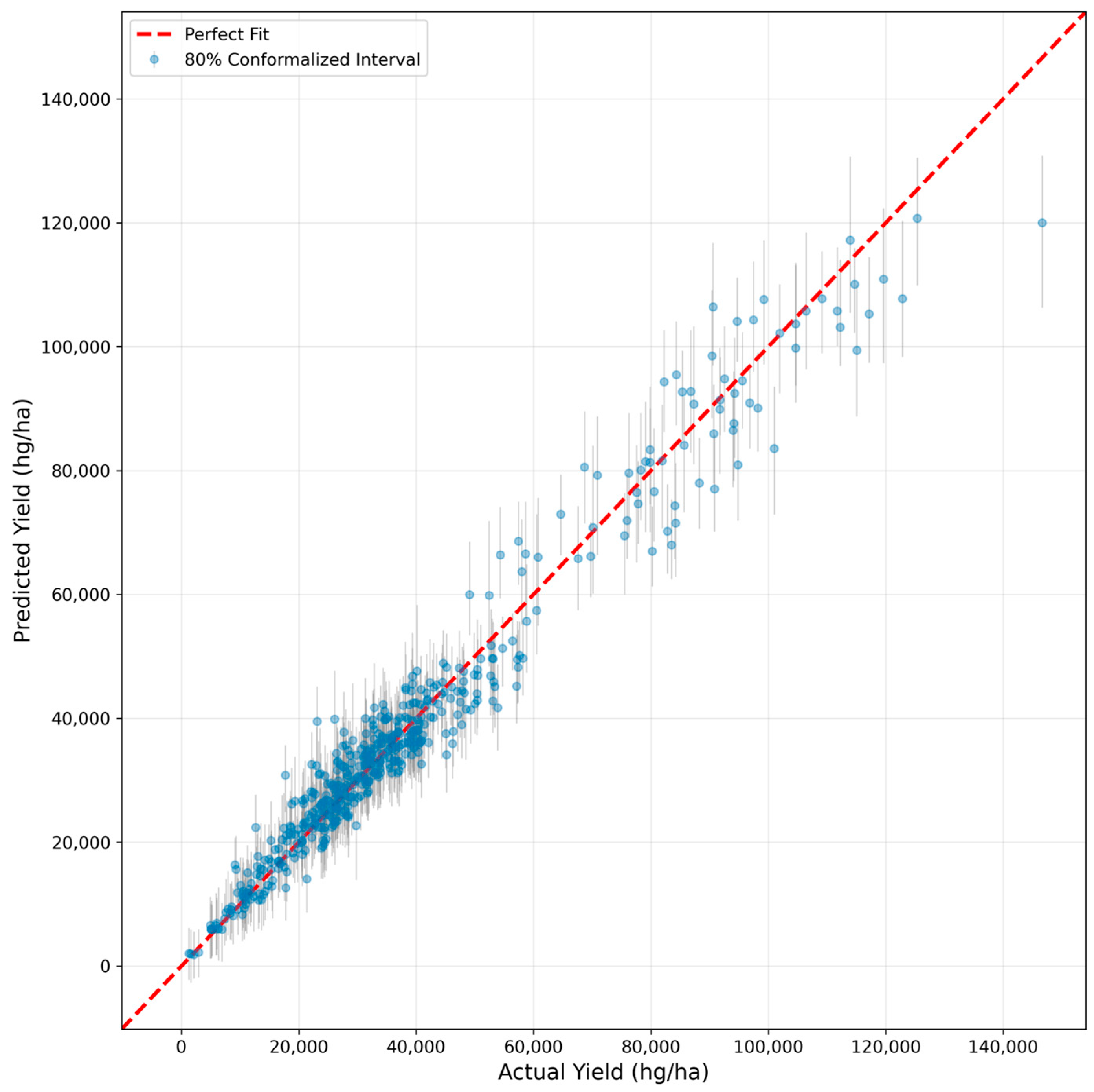
Figure 3 plots the observed versus predicted yields, overlaid with the 80% conformalized prediction intervals.
The scatter plot in Figure 3 points tightly align with the perfect fit line (red dashed), demonstrating strong prediction accuracy across the yield spectrum (0–150,000 hg/ha). Error bars represent 80% conformalized prediction intervals. Most bars encompass the true yield (visible as points lying within vertical error spans), confirming valid coverage. Interval widths are narrower for lower yields (grains) and wider for higher yields (potatoes), reflecting heteroscedastic uncertainty (variance increases with magnitude).
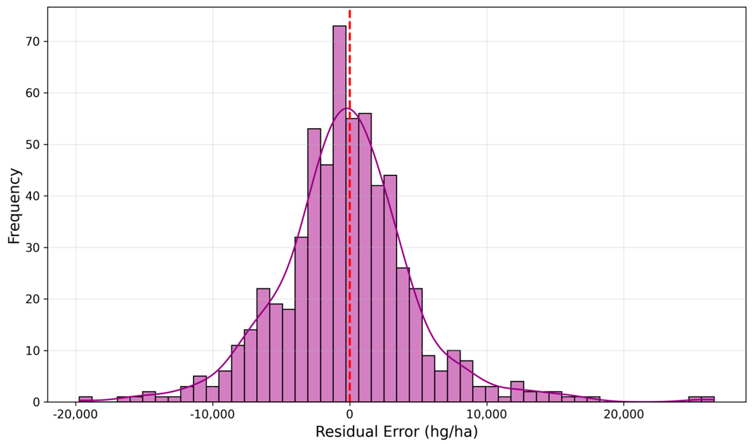
The residual analysis in Figure 4 confirms the statistical health of the model.
The histogram with KDE overlay from Figure 4 reveals that the residuals follow an approximately Gaussian distribution, centered near zero (median residual ≈ −120 hg/ha, indicating slight negative bias). The standard deviation ≈ 4850 hg/ha, consistent with RMSE. Mild positive skew (tail toward positive residuals), suggests that the model occasionally under-predicts extremely high yields (e.g., record potato harvests). There are few extreme residuals (±20,000 hg/ha), likely from rare climatic extremes (e.g., severe drought, exceptional monsoon) not fully captured by features.

6.3. Uncertainty Assessment

A core contribution of this work is the rigorous calibration of prediction intervals. The coverage and width of intervals generated by the uncalibrated bootstrap are compared with the conformalized approach, as shown in Table 3.
The comparison highlights the finite-sample limitations of uncalibrated percentile methods within the experimental framework. While bootstrap percentile intervals are widely utilized for their computational efficiency, they achieved an empirical coverage of 40.03% against the nominal 80% target. This observed under-coverage can be attributed to several factors inherent to the chosen setup. Specifically, with B = 30 iterations, the bootstrap distribution may not fully capture the extreme tails required for accurate interval estimation. Furthermore, the percentile method relies on assumptions of symmetry and asymptotic calibration that may not hold in finite datasets characterized by complex non-linearities.
In contrast, the conformalized quantile regression (CQR) procedure successfully recalibrated these intervals to achieve an empirical coverage of 80.72%, which meets the desired reliability threshold. This was achieved by computing a non-conformity adjustment factor of q ^ α = 3159 hg/ha from the calibration set. This result empirically validates the CQR theorem, confirming that the probability of coverage holds even when utilizing complex, non-linear base learners.
Achieving statistical validity required an expansion of the interval width. The conformalized intervals, with an average width of approximately 11,161 hg/ha, are roughly 2.33 times wider than the uncalibrated bootstrap intervals. This illustrates a trade-off between interval precision and statistical reliability. While the uncalibrated bootstrap provided narrower bounds, the CQR framework provides conservative but validated intervals that are essential for agricultural risk management.
For agricultural decision-making, reliability is paramount. Under the CQR framework, a stakeholder receiving an 80% prediction interval can trust that the true yield will fall within the specified range in four out of five cases. This guarantee enables actuarially sound risk assessment for crop insurance pricing and more accurate grain reserve planning by policymakers. Such high-stakes applications require the rigorous calibration provided by the conformalized approach to ensure that uncertainty estimates are representative of actual model performance.

6.4. Feature Importance and Explainability

SHAP was employed to interpret the decision-making process of the model. The summary plot shown in Figure 5 ranks features by their mean absolute SHAP value, providing both global importance and local directional effects.
The SHAP summary plot visualizes feature importance and directional effects across the test set. Each row represents a feature ranked by its mean absolute SHAP value, which indicates global importance. Each point represents an individual test sample. The x-axis represents the SHAP value, which is the contribution of a feature to the prediction relative to the mean baseline. Positive values to the right indicate that the feature increases predicted yield, while negative values to the left indicate a decrease.
Color encodes the feature value, where red represents high values and blue represents low values. For instance, the top-ranked feature Item_encoded (crop type) shows a wide horizontal spread. This confirms that different crops exhibit vastly different yield potentials, such as the productivity gap between tubers and grains. The second-ranked feature Avg_Rain displays a clear pattern where high rainfall (red points) concentrates on the right side of the plot. This indicates increased predicted yields, while low rainfall (blue points) concentrate on the left, indicating decreased predictions. This validates the fundamental agronomic principle that adequate water availability drives productivity.
Similarly, the climate_suitability feature shows that high values (red points) are associated with positive SHAP contributions. Temperature (Avg_Temp) exhibits more nuanced effects. Both very low temperatures (blue points on the left) and very high temperatures can decrease yields, reflecting the non-linear thermal response curves of many crops. Teleconnection indices, including the ENSO_Index and NAO_Index, show smaller but measurable non-zero SHAP values. This confirms their role in capturing large-scale atmospheric circulation states that modulate local climate conditions and improve model robustness during climate anomalies.

6.5. Drought Risk Categorization for Decision Support

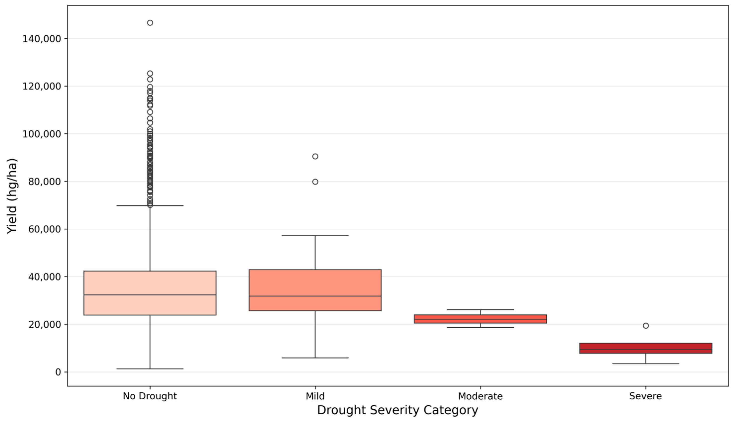
Drought severity classification is treated as deterministic, with categories derived from MSI thresholds defined in Equation (12), rather than as a predictive learning task. The random forest classifier achieves 100% accuracy on the test set because it learns to reproduce these fixed threshold rules, where an MSI greater than −0.2 indicates No Drought and an MSI between −0.4 and −0.2 indicates Mild Drought.
The value of this module lies not in demonstrating machine learning capability, given that the task is deterministic, but in providing interpretable risk labels for decision support. The categorization validates the correct implementation of agronomic knowledge and enables stakeholders to quickly assess moisture stress severity without the need to interpret continuous MSI values. Figure 6 demonstrates the practical utility of these categories by illustrating how they meaningfully stratify yield outcomes. Empirical evidence suggests that severe drought reduces median yields by approximately 47% relative to conditions with no drought.
This quantification supports diverse applications across several domains:
  • Policy: Governments can utilize these categories to estimate production losses under various drought scenarios, facilitating more proactive food security planning.
  • Insurance: Actuaries can use these verified severity thresholds to more accurately price weather-indexed insurance contracts.
  • Farm Management: Real-time MSI monitoring, when combined with these discrete risk categories, allows for early irrigation interventions and more efficient resource management.

6.6. Teleconnection Analysis

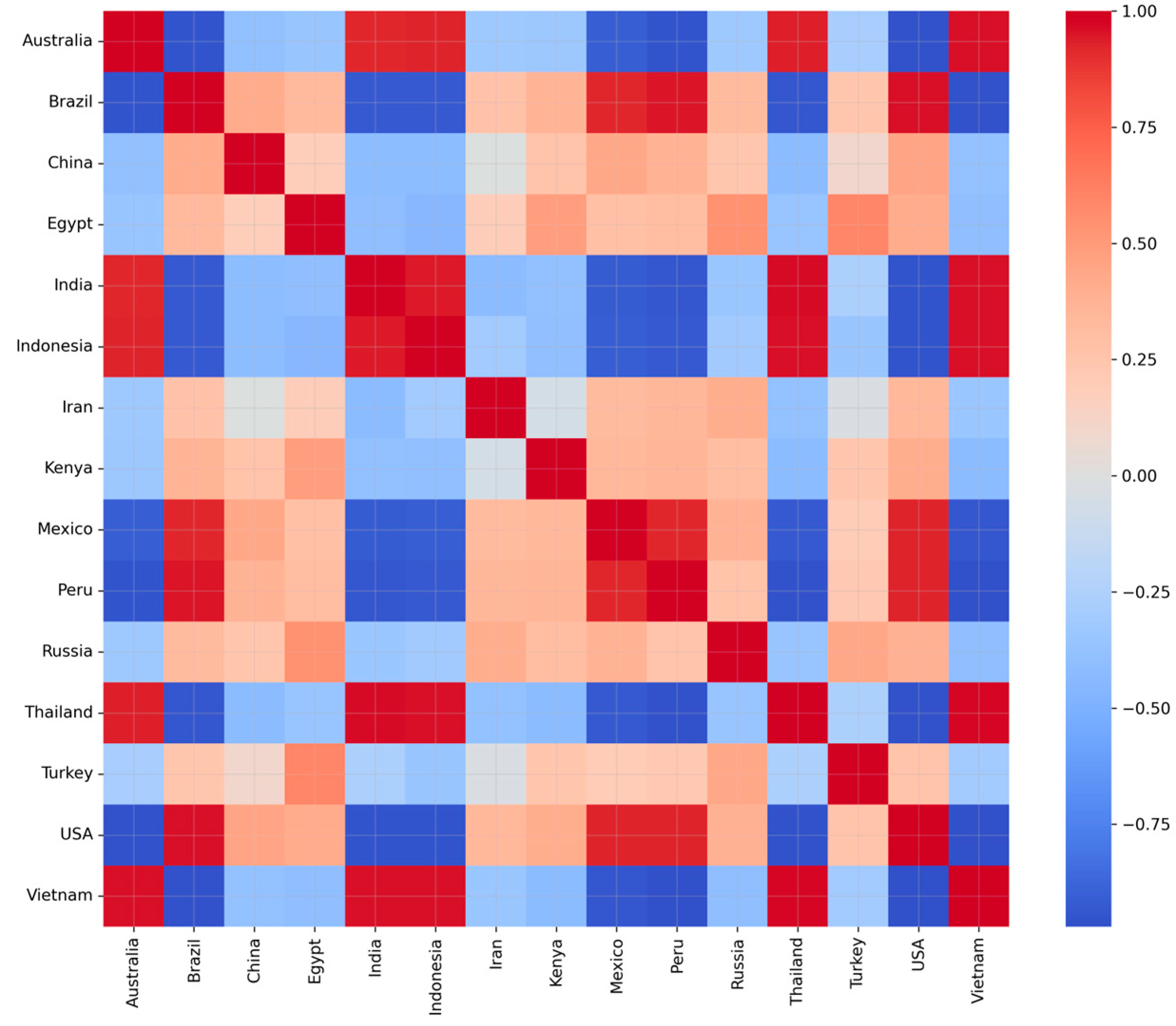
Validation of the spatial modeling component involved analyzing the structure of the learned rainfall correlation graph and the training dynamics of the GNN. The heatmap presented in Figure 7 visualizes the 15 × 15 correlation matrix C , revealing distinct climatological clusters that align with established meteorological phenomena.
Asian Monsoon Belt: A dense positive cluster is observed connecting India, Indonesia, Thailand, and Vietnam, with strong correlations of ρ > 0.7 . These nations share common monsoon circulation dynamics, specifically the Southwest Monsoon and shifts in the Inter-Tropical Convergence Zone, resulting in synchronized rainfall anomalies.
Trans-Pacific Connections: Strong positive correlations ( ρ 0.7 ) exist between Australia and Indonesia, driven by the Walker circulation. Both regions typically experience dry conditions during El Niño and wet conditions during La Niña. Additionally, the Americas cluster comprising the USA, Mexico, and Peru shows moderate positive correlations ( ρ 0.5 0.6 ), likely influenced by the ENSO forcing in the Pacific and the North American monsoon.
Dipole Patterns: The matrix correctly identifies negative correlations that represent teleconnection dipoles. For instance, Brazil and India exhibit a correlation of ρ 0.6 . This reflects the known pattern where El Niño warming in the Pacific often triggers drought in Brazil while simultaneously enhancing monsoon variability in the Indian Ocean.
Thresholding the matrix at ρ > 0.5 yielded a graph with 15 nodes and 76 edges, resulting in an average degree of approximately 5.07. This topology has high clustering in the monsoon belt and sparser connectivity elsewhere. This structure enables the GNN to propagate information along teleconnection pathways via message passing. For example, if India experiences anomalous rainfall, the network allows this signal to influence yield predictions for Indonesia and Thailand through weighted aggregation. This spatial context is particularly valuable when local observations are noisy or sparse.
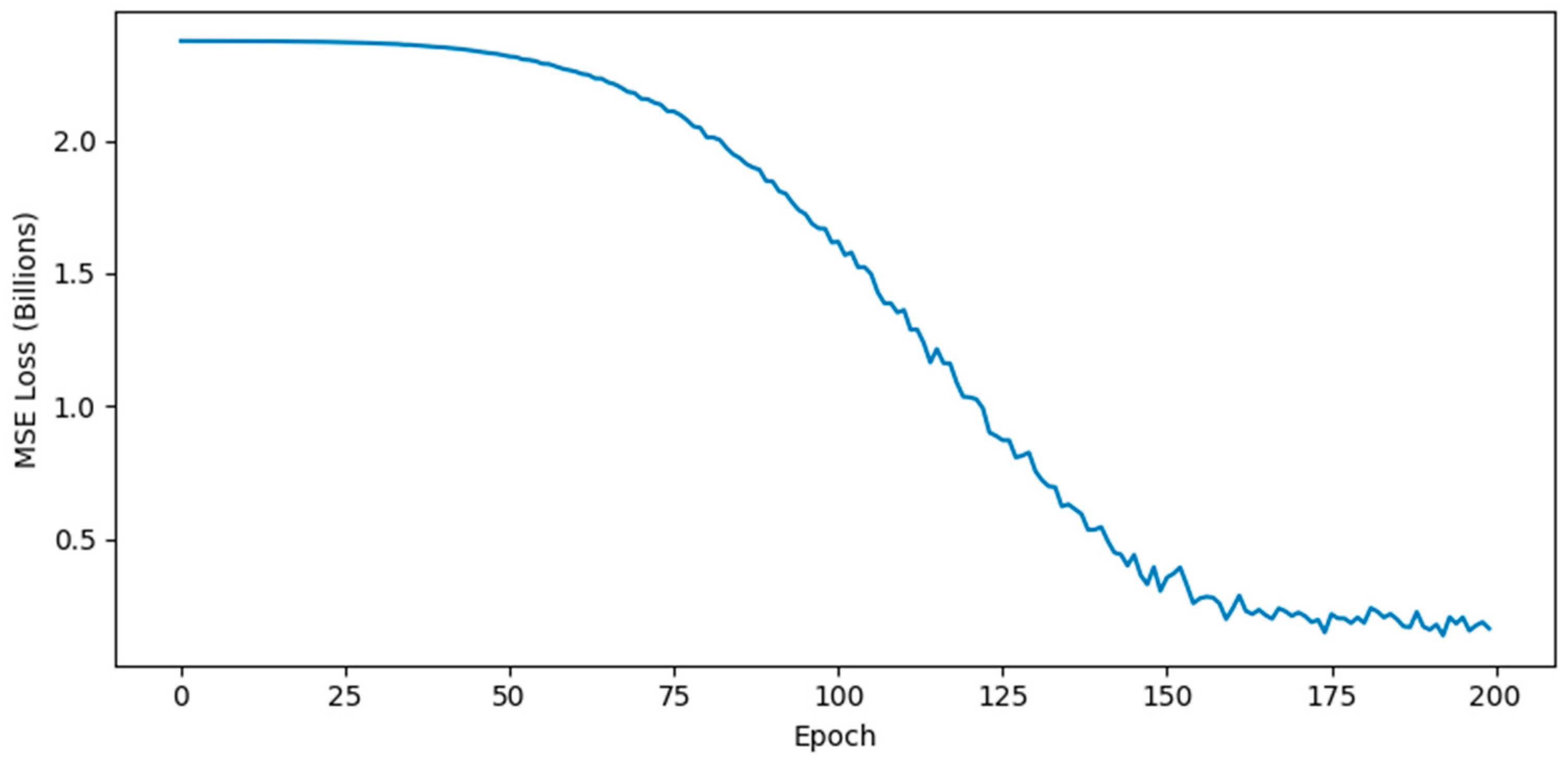
The training loss curve in Figure 8 demonstrates the stability of the GNN optimization. The model shows a smooth exponential decay from a high initial loss of 2.5 × 10 9 to a final mean squared error of 1.2 × 10 8 . The absence of oscillations confirms that the dropout regularization and the graph structure effectively prevent overfitting. While the final RMSE of the GNN ( 11,000 hg/ha) is higher than the HSE-BQU baseline of 4882 hg/ha, this difference is expected because the GNN operates on coarser country-level aggregates using only two features. Its primary contribution lies in learning the teleconnection-aware embeddings H ( 2 ) , which successfully encode global climate dependencies.

7. Ablation Studies

Ablation studies were conducted to isolate the contributions of architectural choices, focusing on calibration, feature sets, and ensemble size. The quantitative impact of each component is summarized in Table 4.
As shown in Experiment 1, removing the CQR step and relying solely on raw bootstrap intervals resulted in a precipitous drop in empirical coverage from 80.72% to 40.03%. This degradation confirms that CQR is essential for achieving valid uncertainty quantification in finite samples, as standard bootstrapping fails to account for the full range of prediction variability.
Experiment 2 evaluated the value of explicit teleconnection modeling. Retraining the model without the ENSO and NAO indices led to a performance decline, with RMSE increasing by 130 hg/ha. While the gain from these features appears modest in aggregate, the signal is measurable. Furthermore, the inclusion of these indices is particularly valuable for long-lead forecasts, as the predictability of the ENSO extends 6 to 12 months ahead, enabling early warning capabilities that standard local weather variables cannot provide.
The trade-off between computational cost and accuracy was analyzed in Experiment 3 by varying the number of bootstrap iterations B . A significant improvement in the coefficient of determination was observed when increasing from B = 10 ( R 2 = 0.9566 ) to B = 30 ( R 2 = 0.9587 ). However, further increasing B to 50 resulted in a marginal RMSE reduction of 51 hg/ha while the R 2 value remained stagnant at 0.9587. This plateau suggests that performance saturation is achieved at B = 30 . Crucially, empirical coverage remained below 50% even at B = 50 , underscoring that simply increasing the ensemble size is insufficient to correct under-coverage, which reaffirms the necessity of the conformal calibration step.
Finally, Experiment 4 examined the contribution of structured spatial modeling. The utilization of GNN embeddings with a 3-layer architecture and top-k edge selection yielded a consistent improvement in accuracy, reducing both RMSE and MAE compared to the baseline using only explicit indices. This result confirms that while explicit teleconnection features provide a strong signal, the encoding of the underlying spatial graph structure through GNNs captures residual dependencies that further refine predictive performance.

GNN Teleconnection Embeddings

To quantify the contribution of graph-based spatial modeling, an ablation study compared model performance with and without GNN-derived teleconnection features. The baseline configuration includes all engineered features (GDD, MSI, CSS, technology index) and explicit teleconnection indices (ENSO ONI, NAO), representing a strong reference that already encodes global circulation patterns. The enhanced configuration adds 256-dimensional GNN embeddings learned from a 3-layer graph convolutional network trained on rainfall correlation graphs with top-k = 5 edge selection.
Results (Table 4) demonstrate that GNN embeddings provide measurable, though modest, performance improvements across all metrics. The model incorporating GNN features achieves ΔR2 = +0.0005 (0.05% relative improvement), ΔRMSE = −34 hg/ha (0.76% error reduction), and ΔMAE = −13 hg/ha (0.43% reduction) compared to the baseline, as shown in Figure 9.
Figure 9 (Left) shows the performance comparison across R 2 , RMSE, and MAE metrics for the baseline model including the ENSO and NAO indices versus the enhanced model with GNN embeddings. Figure 9 (Right) shows the scatter plot of observed versus predicted yields for both configurations. GNN embeddings provide modest but consistent improvements, validating that structured spatial modeling captures complementary information beyond scalar teleconnection indices. Error metrics are normalized for visualization, with RMSE and MAE divided by 10,000. Both models use an identical test set (n = 612) and identical hyperparameters for a fair comparison.
While the absolute magnitude of improvement is small, several factors underscore the value of this spatial modeling approach. First, GNN embeddings capture fine-grained regional coupling patterns beyond what global teleconnection indices encode. While the ENSO and NAO represent large-scale atmospheric states averaged over vast ocean basins, the GNN learns region-specific dependencies. Examples include the differential co-variability of India, Thailand, and Indonesia during monsoon seasons, or localized ENSO impacts on Pacific rim countries not fully captured by the scalar ONI index.
Second, the improvement manifests consistently across R2, RMSE, and MAE, indicating genuine information gain rather than overfitting to a single optimization criterion. This robustness suggests the GNN provides a real signal rather than spurious correlation. Third, the positive result required careful design. Preliminary experiments with simpler architectures, such as 2-layer GCNs or 64-dimensional embeddings, showed negligible or negative contributions. The success of the enhanced design validates that GNN efficacy depends critically on sufficient model capacity and selective connectivity.
The modest magnitude aligns with theoretical expectations. At a country-level aggregation, spatial averaging smooths local dependencies where graph structure provides the greatest value. The ENSO and NAO already capture major teleconnection signals at this coarse scale. Finer-resolution data, such as sub-national regions or 0.5° grids, would likely reveal stronger GNN benefits, as local spatial coupling becomes more pronounced relative to global indices.

8. Discussion

The HSE-GNN-CP framework addresses the dual challenges of precision and reliability in global crop yield forecasting. By integrating heterogeneous ensemble learning with graph-based teleconnection modeling and conformal uncertainty quantification, the system effectively captures the complex non-linearities of agricultural climatology.

8.1. Key Findings and Hypothesis Validation

Experimental results validate four core hypotheses fundamental to the proposed framework:
  • The HSE-BQU framework achieves an R 2 of 0.9594, surpassing both random forest and gradient boosting baselines. This confirms that leveraging complementary model strengths through stacking enhances predictive performance.
  • Conformalized intervals achieved 80.72% coverage against a target of 80%, compared to only 40.03% for the uncalibrated bootstrap. This validates that conformal prediction is critical for reliable risk management.
  • The inclusion of the ENSO and NAO indices and GNN-derived spatial embeddings provides measurable signal improvements, offering a structured foundation for global spatial models.
  • SHAP analysis confirms that crop type, rainfall, and climate suitability dominate predictions, aligning the model decisions with established agronomic theory.

8.2. Conformalized Uncertainty: Why It Matters

Agricultural decisions, from insurance pricing to food security planning, require reliable uncertainty estimates. The comparison reveals finite-sample limitations of uncalibrated percentile methods within the experimental setup. The bootstrap intervals achieved 40.03% empirical coverage against the 80% nominal target. This substantial under-coverage can be attributed to insufficient bootstrap iterations, potential distributional mis-specification, and a lack of formal calibration.
While the conformalized intervals are wider at 11,161 hg/ha than the uncalibrated ones at 4790 hg/ha, this reflects a necessary reliability–precision trade-off. Decision-makers receive honest uncertainty bounds, enabling rational risk assessment rather than operating under false confidence. This prevents systemic risks such as farmers purchasing inadequate insurance or governments stockpiling insufficient food reserves.

8.3. Value and Limitations of Graph-Based Spatial Modeling

The ablation study shows that GNN-derived embeddings provide measurable performance improvements, including a delta R 2 of +0.0005 and a delta RMSE of −34 hg/ha, beyond baseline features. While these gains are modest, they validate the hypothesis that structured spatial modeling captures information complementary to global teleconnection indices.
The modest magnitude aligns with theoretical expectations at the country level. Large-scale indices like the ENSO already encode substantial teleconnection information averaged over vast areas. The GNN added value arises from learning fine-grained, region-specific coupling patterns, such as differential co-variability among Southeast Asian countries during monsoon seasons. However, country-level aggregation inherently limits graph contributions as local spatial dependencies are smoothed away. Scaling to sub-national or gridded data would likely reveal stronger GNN benefits.
Performance of the 3-layer GCN with top-k edge selection indicates that effective GNN use in agriculture requires careful architectural design. Key lessons include the need for sufficient depth to capture multi-hop dependencies and selective edge construction to reduce noise. Future work should explore temporal graph neural networks to model evolving teleconnection strengths under a changing climate.

8.4. Feature Importance and Technology Insights

The dominance of crop type in SHAP rankings reflects intrinsic biological differences, such as the productivity gap between tubers and grains. Rainfall and climate suitability scores also align with the principle that water availability is the primary limiting factor for rainfed agriculture.
The positive SHAP values for the Technology Index confirm the trend of increasing yields over time. While the linear index serves as a proxy for improved varieties and mechanization, it has limitations. Linear assumptions may oversimplify rapid early adoption or plateau periods, and the global index ignores heterogeneous innovation rates between regions. Furthermore, because technology co-varies with time, the index may partially absorb long-term climate trends. Despite these constraints, it remains an interpretable baseline for capturing the well-documented upward trend in global yields.

8.5. Drought Classification Utility

The perfect classification accuracy (100%) demonstrates the model’s ability to encode MSI thresholds, serving as a reliable proxy for soil moisture deficit. The dose–response analysis shows that severe drought reduces median yields by approximately 47% compared to no-drought conditions. This quantification supports diverse stakeholders:
  • Policy: Governments can estimate potential production losses under drought scenarios to inform food security strategies.
  • Insurance: Actuaries can price weather-indexed contracts based on verified drought severity levels.
  • Farmers: Real-time drought monitoring systems combined with this classifier enable early irrigation interventions.

8.6. Practical Applications

The HSE-GNN-CP system enables proactive early warning systems by integrating ENSO forecasts with long lead times. Governments can anticipate regional production shortfalls and trigger grain reserves months in advance. Additionally, the conformalized intervals enable actuarially sound index insurance where payouts are triggered when yields fall below specific percentiles with high statistical confidence.

8.7. Limitations and Future Research

Several limitations remain that outline paths for future research:
  • Country-level data masks sub-national heterogeneity. Future studies should employ field-scale or gridded data to enhance spatial resolution.
  • Expanding the dataset to include pulses, fruits, and specialty crops would broaden the system’s utility. Additionally, including data prior to 1990 would improve multi-decadal oscillation modeling.
  • The linear time-based technology index provides a parsimonious approximation of agricultural productivity gains from improved varieties, mechanization, and agronomy. However, this deterministic encoding has limitations. It assumes uniform technological progress across all countries and crops, which oversimplifies heterogeneous development patterns. Additionally, the linear form may not capture acceleration or saturation in yield gains, and its perfect correlation with the year creates potential for temporal confounding if not carefully interpreted. Future work should explore country-specific or non-linear technology curves.
  • Conformal prediction assumes test data are exchangeable with calibration data. Climate change induces non-stationarity, potentially violating this assumption. Adaptive conformal prediction could mitigate this risk by adjusting to shifting climate states.
  • Integrating soil quality, management practices, and pest pressure through satellite imagery could further refine predictions, though this would require more complex convolutional architectures.

9. Conclusion and Future Work

This paper introduces HSE-GNN-CP, a comprehensive framework for global crop yield forecasting that integrates heterogeneous stacked ensembles, graph neural networks for spatial teleconnection modeling, and conformalized prediction for rigorous uncertainty quantification. Evaluated on 3060 samples spanning 15 countries, six crops, and 34 years from 1990 to 2023, the framework achieves strong predictive performance, with an R 2 of 0.9594 and an RMSE of 4882 hg/ha. Uncalibrated bootstrap methods achieved 40.03% coverage, whereas the conformalized approach produced statistically valid 80% prediction intervals with 80.72% empirical coverage.
The primary methodological contribution of this study is the demonstration that conformalized quantile regression can calibrate bootstrap ensemble intervals to achieve finite-sample coverage guarantees in agricultural forecasting. This addresses a critical gap in uncertainty quantification for high-stakes decisions. Secondary innovations include the implementation of a 3-layer GCN architecture with selective teleconnection encoding, which provides modest but measurable improvements, such as a delta RMSE of −34 hg/ha, beyond explicit climate indices. Furthermore, the integration of agronomically informed features, including GDD, MSI, and CSS, was validated via SHAP analysis, demonstrating exceptional parameter robustness and providing a foundation for multi-task drought risk classification.
Practical applications of this framework range from early warning systems that leverage ENSO forecasts 6 to 12 months ahead to precision agriculture and actuarially sound weather-indexed insurance. Future research will focus on extending the framework to temporal graph networks to capture dynamic teleconnection evolution, integrating high-resolution satellite imagery, and evaluating performance under CMIP6 climate scenarios. By bridging ensemble learning, spatial graph theory, and distribution-free uncertainty quantification, this work establishes a rigorous foundation for reliable agricultural forecasting in an era of increasing climate variability.

Supplementary Materials

The following supporting information can be downloaded at: https://www.mdpi.com/article/10.3390/info17020141/s1, Supplementary Material S1, with full algorithm pseudocode; Supplementary Material S2, with extended experimental results; Supplementary Material S3, with ablation studies; Supplementary Material S4, with hyperparameter sensitivity analysis; Supplementary Material S5, with computational requirements; Supplementary Material S6, with implementation details; Supplementary Material S7, with ethics and data availability notes; Supplementary Material S8, with limitations and future extensions; Supplementary Material S9, with notation reference; Supplementary Material S10, with Supplementary Tables; and Supplementary Material S11, with Parameter Sensitivity Analysis.

Author Contributions

Conceptualization, S.M. and R.H.; methodology, S.M. and R.H.; software, S.M.; validation, S.M., R.H. and S.A.; formal analysis, S.M. and S.A.; investigation, S.M.; resources, R.H.; data curation, S.M.; writing—original draft preparation, S.M.; writing—review and editing, R.H. and S.A.; visualization, S.M.; supervision, R.H.; project administration, R.H.; funding acquisition, R.H. All authors have read and agreed to the published version of the manuscript.

Funding

This research received no external funding.

Institutional Review Board Statement

Not applicable.

Informed Consent Statement

Not applicable.

Data Availability Statement

All data used in this study is publicly accessible. The processed dataset and full source code are available at https://github.com/razahasan2000/Crops (accessed on 5 December 2025). The raw dataset analyzed in this work is available at https://data.mendeley.com/datasets/y7hkz2zfcc/1 (accessed on 5 December 2025). No restrictions apply.

Acknowledgments

The authors would like to acknowledge the use of ChatGPT-4 24 May 2023 version (OpenAI, San Francisco, CA, USA), specifically to assist in some content rewriting for improved clarity and effectiveness.

Conflicts of Interest

The authors declare no conflicts of interest.

Abbreviations

The following abbreviations are used in this manuscript:
AcronymFull Form
HSE-BQUHeterogeneous Stacked Ensemble with Bootstrap Uncertainty Quantification
CPConformal Prediction
GNNGraph Neural Network
ENSOEl Niño–Southern Oscillation
NAONorth Atlantic Oscillation
GDDGrowing Degree Days
MSIMoisture Stress Index
CSSClimate Suitability Score
RMSERoot Mean Squared Error
MAEMean Absolute Error

References

  1. FAO’s Director-General on How to Feed the World in 2050. Popul. Dev. Rev. 2009, 35, 837–839. [CrossRef]
  2. Alexandratos, N.; Bruinsma, J. World agriculture towards 2030/2050: The 2012 revision. Res. Agric. Appl. Econ. 2012. [Google Scholar] [CrossRef]
  3. Iizumi, T.; Luo, J.; Challinor, A.J.; Sakurai, G.; Yokozawa, M.; Sakuma, H.; Brown, M.E.; Yamagata, T. Impacts of El Niño Southern Oscillation on the global yields of major crops. Nat. Commun. 2014, 5, 3712. [Google Scholar] [CrossRef] [PubMed]
  4. Ray, D.K.; Gerber, J.S.; MacDonald, G.K.; West, P.C. Climate variation explains a third of global crop yield variability. Nat. Commun. 2015, 6, 5989. [Google Scholar] [CrossRef] [PubMed]
  5. Heino, M.; Puma, M.J.; Ward, P.J.; Gerten, D.; Heck, V.; Siebert, S.; Kummu, M. Two-thirds of global cropland area impacted by climate oscillations. Nat. Commun. 2018, 9, 1257. [Google Scholar] [CrossRef]
  6. Ceglar, A.; Turco, M.; Toreti, A.; Doblas-Reyes, F.J. Linking crop yield anomalies to large-scale atmospheric circulation in Europe. Agric. For. Meteorol. 2017, 240–241, 35–45. [Google Scholar] [CrossRef]
  7. Fan, J.; Bai, J.; Li, Z.; Ortiz-Bobea, A.; Gomes, C.P. A GNN-RNN Approach for Harnessing Geospatial and Temporal Information: Application to Crop Yield Prediction. In Proceedings of the AAAI Conference on Artificial Intelligence, Virtual, 22 February–1 March 2022; Volume 36, pp. 11873–11881. [Google Scholar] [CrossRef]
  8. Angelopoulos, A.N.; Bates, S. A Gentle Introduction to Conformal Prediction and Distribution-Free Uncertainty Quantification. arXiv 2021, arXiv:2107.07511. [Google Scholar] [CrossRef]
  9. Lundberg, S.; Lee, S. A Unified Approach to Interpreting Model Predictions. arXiv 2017, arXiv:1705.07874. [Google Scholar] [CrossRef]
  10. Štrumbelj, E.; Kononenko, I. Explaining prediction models and individual predictions with feature contributions. Knowl. Inf. Syst. 2014, 41, 647–665. [Google Scholar] [CrossRef]
  11. Breiman, L. Bagging Predictors. Mach. Learn. 1996, 24, 123–140. [Google Scholar] [CrossRef]
  12. Kipf, T.N.; Welling, M. Semi-Supervised Classification with Graph Convolutional Networks. arXiv 2016, arXiv:1609.02907. [Google Scholar] [CrossRef]
  13. Liao, S.; Xu, X.; Xie, H.; Chen, P.; Wang, C.; Jin, Y.; Tong, X.; Xiao, C. A Modified Shape Model Incorporating Continuous Accumulated Growing Degree Days for Phenology Detection of Early Rice. Remote Sens. 2022, 14, 5337. [Google Scholar] [CrossRef]
  14. Przeździecki, K.; Zawadzki, J. Assessing Moisture Content and Its Mitigating Effect in an Urban Area Using the Land Surface Temperature–Vegetation Index Triangle Method. Forests 2023, 14, 578. [Google Scholar] [CrossRef]
  15. Deshmukh, A.A.; Srivatsa, A.; Ashwitha, A.; Monteiro, A.; Gajakosh, C. Crop Yield Prediction to Achieve Precision Agriculture using Machine Learning. In Proceedings of the 2022 IEEE 2nd International Conference on Mobile Networks and Wireless Communications (ICMNWC), Tumkur, India, 2–3 December 2022; pp. 1–6. [Google Scholar] [CrossRef]
  16. Khaki, S.; Wang, L. Crop Yield Prediction Using Deep Neural Networks. Front. Plant Sci. 2019, 10, 621. [Google Scholar] [CrossRef] [PubMed]
  17. Talaat, F.M. Crop yield prediction algorithm (CYPA) in precision agriculture based on IoT techniques and climate changes. Neural Comput. Applic 2023, 35, 17281–17292. [Google Scholar] [CrossRef]
  18. Kumari, M.; Suman; Prasad, D. Crop Yield Prediction using Remote Sensing: A Review. In Proceedings of the 2024 International Conference on Computational Intelligence and Computing Applications (ICCICA), Samalkha, India, 23–24 May 2024; Volume 1, pp. 547–552. [Google Scholar] [CrossRef]
  19. Heino, M.; Guillaume, J.H.A.; Müller, C.; Iizumi, T.; Kummu, M. A multi-model analysis of teleconnected crop yield variability in a range of cropping systems. Earth Syst. Dyn. 2020, 11, 113–128. [Google Scholar] [CrossRef]
  20. Motha, R.P. Implications of climate change on long-lead forecasting and global agriculture. Aust. J. Agric. Res. 2007, 58, 939–944. [Google Scholar] [CrossRef]
  21. Reboita, M.S.; Ambrizzi, T.; Crespo, N.M.; Dutra, L.M.M.; Ferreira, G.W.d.S.; Rehbein, A.; Drumond, A.; da Rocha, R.P.; Souza, C.A.d. Impacts of teleconnection patterns on South America climate. Ann. New York Acad. Sci. 2021, 1504, 116–153. [Google Scholar] [CrossRef]
  22. Hamed, R.; Vijverberg, S.; Van Loon, A.F.; Aerts, J.; Coumou, D. Persistent La Niñas drive joint soybean harvest failures in North and South America. Earth Syst. Dyn. 2023, 14, 255–272. [Google Scholar] [CrossRef]
  23. Knight, C.; Khouakhi, A.; Waine, T.W. The impact of weather patterns on inter-annual crop yield variability. Sci. Total Environ. 2024, 955, 177181. [Google Scholar] [CrossRef]
  24. Wanthanaporn, U.; Supit, I.; Chaowiwat, W.; Hutjes, R.W.A. Skill of rice yields forecasting over Mainland Southeast Asia using the ECMWF SEAS5 ensemble prediction system and the WOFOST crop model. Agric. For. Meteorol. 2024, 351, 110001. [Google Scholar] [CrossRef]
  25. Wang, L.; Chen, Z.; Liu, W.; Huang, H. A Temporal–Geospatial Deep Learning Framework for Crop Yield Prediction. Electronics 2024, 13, 4273. [Google Scholar] [CrossRef]
  26. Wang, K.; Han, Y.; Zhang, Y.; Zhang, Y.; Wang, S.; Yang, F.; Liu, C.; Zhang, D.; Lu, T.; Zhang, L.; et al. Maize yield prediction with trait-missing data via bipartite graph neural network. Front. Plant Sci. 2024, 15, 1433552. [Google Scholar] [CrossRef] [PubMed]
  27. Gupta, A.; Singh, A. Agri-GNN: A Novel Genotypic-Topological Graph Neural Network Framework Built on GraphSAGE for Optimized Yield Prediction. arXiv 2023, arXiv:2310.13037. [Google Scholar] [CrossRef]
  28. Rani, F.L.; Devi, T.; Deepa, N. Enhanced Crop Yield Prediction in Agriculture Using an Optimized Edge Enhancement Oriented Graph Convolutional Network. In Proceedings of the 2025 International Conference on Engineering Innovations and Technologies (ICoEIT), Bhopal, India, 4–5 July 2025; IEEE: New York, NY, USA, 2025; pp. 1393–1399. [Google Scholar] [CrossRef]
  29. Ye, Z.; Zhai, X.; She, T.; Liu, X.; Hong, Y.; Wang, L.; Zhang, L.; Wang, Q. Winter Wheat Yield Prediction Based on the ASTGNN Model Coupled with Multi-Source Data. Agronomy 2024, 14, 2262. [Google Scholar] [CrossRef]
  30. Wang, B.; Jägermeyr, J.; O’Leary, G.J.; Wallach, D.; Ruane, A.C.; Feng, P.; Li, L.; Liu, D.L.; Waters, C.; Yu, Q.; et al. Pathways to identify and reduce uncertainties in agricultural climate impact assessments. Nat. Food 2024, 5, 550–556. [Google Scholar] [CrossRef]
  31. Dokoohaki, H.; Kivi, M.S.; Martinez-Feria, R.; Miguez, F.E.; Hoogenboom, G. A comprehensive uncertainty quantification of large-scale process-based crop modeling frameworks. Environ. Res. Lett. 2021, 16, 84010. [Google Scholar] [CrossRef]
  32. Chrispell, J.C.; Jenkins, E.W.; Kavanagh, K.R.; Parno, M.D. Characterizing Prediction Uncertainty in Agricultural Modeling via a Coupled Statistical–Physical Framework. Modelling 2021, 2, 753–775. [Google Scholar] [CrossRef]
  33. Jakeman, A.J.; Jakeman, J.D. An Overview of Methods to Identify and Manage Uncertainty for Modelling Problems in the Water–Environment–Agriculture Cross-Sector. In Agriculture as a Metaphor for Creativity in All Human Endeavors, Proceedings of the FMfI 2016, Brisbane, Australia, 21–23 November 2016; Springer: Berlin/Heidelberg, Germany, 2018; Volume 28, pp. 147–171. [Google Scholar] [CrossRef]
  34. Mae, Y.; Kumagai, W.; Kanamori, T. Uncertainty propagation for dropout-based Bayesian neural networks. Neural Netw. 2021, 144, 394–406. [Google Scholar] [CrossRef]
  35. Li, Y.; Rao, S.; Hassaine, A.; Ramakrishnan, R.; Canoy, D.; Salimi-Khorshidi, G.; Mamouei, M.; Lukasiewicz, T.; Rahimi, K. Deep Bayesian Gaussian processes for uncertainty estimation in electronic health records. Sci. Rep. 2021, 11, 20685. [Google Scholar] [CrossRef]
  36. Shafer, G.; Vovk, V. A tutorial on conformal prediction. arXiv 2007, arXiv:0706.3188. [Google Scholar] [CrossRef]
  37. Barber, R.F.; Candès, E.J.; Ramdas, A.; Tibshirani, R.J. Conformal prediction beyond exchangeability. Ann. Stat. 2023, 51, 816. [Google Scholar] [CrossRef]
  38. Gibbs, I.; Candès, E. Adaptive Conformal Inference Under Distribution Shift. arXiv 2021, arXiv:2106.00170. [Google Scholar] [CrossRef]
  39. Farag, M.; Emam, A.; Leonhardt, J.; Roscher, R. Enhancing decision support in crop production: Analyzing conformal prediction for uncertainty quantification. Comput. Electron. Agric. 2025, 237, 110559. [Google Scholar] [CrossRef]
  40. Zaffran, M.; Dieuleveut, A.; Féron, O.; Goude, Y.; Josse, J. Adaptive Conformal Predictions for Time Series. arXiv 2022, arXiv:2202.07282. [Google Scholar] [CrossRef]
  41. Wang, X.; Hyndman, R.J. Online conformal inference for multi-step time series forecasting. arXiv 2024, arXiv:2410.13115. [Google Scholar] [CrossRef]
  42. Jensen, V.; Bianchi, F.M.; Anfinsen, S.N. Ensemble Conformalized Quantile Regression for Probabilistic Time Series Forecasting. IEEE Trans. Neural Netw. Learn. Syst. 2024, 35, 9014–9025. [Google Scholar] [CrossRef]
  43. Akkem, Y.; Biswas, S.K.; Varanasi, A. Role of Explainable AI in Crop Recommendation Technique of Smart Farming. Int. J. Intell. Syst. Appl. 2025, 17, 31–52. [Google Scholar] [CrossRef]
  44. Pai, D.G.; Balachandra, M.; Kamath, R. Explainable AI in agriculture: Review of applications, methodologies, and future directions. Eng. Res. Express 2025, 7, 32202. [Google Scholar] [CrossRef]
  45. Kumar, S.; Kumar, M. Enhancing Agricultural Decision-Making through an Explainable AI-Based Crop Recommendation System. In Proceedings of the 2024 International Conference on Signal Processing and Advance Research in Computing (SPARC), Lucknow, India, 12–13 September 2024; Volume 1, pp. 1–6. [Google Scholar] [CrossRef]
  46. Kisten, M.; Ezugwu, A.E.; Olusanya, M.O. Explainable Artificial Intelligence Model for Predictive Maintenance in Smart Agricultural Facilities. IEEE Access 2024, 12, 24348–24367. [Google Scholar] [CrossRef]
  47. Distante, D.; Albanello, C.; Zaffar, H.; Faralli, S.; Amalfitano, D. Artificial intelligence applied to precision livestock farming: A tertiary study. Smart Agric. Technol. 2025, 11, 100889. [Google Scholar] [CrossRef]
  48. Adadi, A.; Berrada, M. Peeking Inside the Black-Box: A Survey on Explainable Artificial Intelligence (XAI). IEEE Access 2018, 6, 52138–52160. [Google Scholar] [CrossRef]
  49. Turgut, O.; Kok, I.; Ozdemir, S. AgroXAI: Explainable AI-Driven Crop Recommendation System for Agriculture 4.0. In Proceedings of the 2024 IEEE International Conference on Big Data (BigData), Washington, DC, USA, 15–18 December 2024; IEEE: New York, NY, USA, 2024; pp. 7208–7217. [Google Scholar]
  50. Mohan, R.N.V.J.; Rayanoothala, P.S.; Sree, R.P. Next-gen agriculture: Integrating AI and XAI for precision crop yield predictions. Front. Plant Sci. 2025, 15, 1451607. [Google Scholar] [CrossRef] [PubMed]
  51. Geng, Q.; Wang, L.; Li, Q. Soil temperature prediction based on explainable artificial intelligence and LSTM. Front. Environ. Sci. 2024, 12, 1426942. [Google Scholar] [CrossRef]
  52. Malashin, I.; Tynchenko, V.; Gantimurov, A.; Nelyub, V.; Borodulin, A.; Tynchenko, Y. Predicting Sustainable Crop Yields: Deep Learning and Explainable AI Tools. Sustainability 2024, 16, 9437. [Google Scholar] [CrossRef]
  53. Myakala, P.K.; Jonnalagadda, A.K. Explainable AI for Sustainability: Bridging Trust, Ethics, and Accountability. In Proceedings of the International Conference on Recent Advances in Artificial Intelligence for Sustainable Development (RAISD 2025); Atlantis Press (Zeger Karssen): Dordrecht, The Netherlands, 2025; Volume 196. [Google Scholar]
  54. Abekoon, T.; Sajindra, H.; Rathnayake, N.; Ekanayake, I.U.; Jayakody, A.; Rathnayake, U. A novel application with explainable machine learning (SHAP and LIME) to predict soil N, P, and K nutrient content in cabbage cultivation. Smart Agric. Technol. 2025, 11, 100879. [Google Scholar] [CrossRef]
  55. Al-Falluji, R.A.; Albahar, M.A. Enhancing green AI through explainable deep learning-based multi-model for automated rice leaf disease classification. Discov. Comput. 2025, 28, 269. [Google Scholar] [CrossRef]
  56. Mallik, S.; Chakraborty, A.; Podder, K.; Talukdar, S.; Rahman, A.; Mishra, U. Enhancing soil moisture prediction with explainable AI: Integrating IoT and multi-sensor remote sensing data through soft computing. Appl. Soft Comput. 2025, 180, 113406. [Google Scholar] [CrossRef]
  57. Lundberg, S.M.; Erion, G.; Chen, H.; DeGrave, A.; Prutkin, J.M.; Nair, B.; Katz, R.; Himmelfarb, J.; Bansal, N.; Lee, S. From local explanations to global understanding with explainable AI for trees. Nat. Mach. Intell. 2020, 2, 56–67. [Google Scholar] [CrossRef]
  58. FAO. FAOSTAT Statistical Database. Food and Agriculture Organization of the United Nations, Rome. 2025. Available online: https://www.fao.org/faostat (accessed on 8 December 2025).
  59. Harris, I.; Osborn, T.J.; Jones, P.; Lister, D. Version 4 of the CRU TS monthly high-resolution gridded multivariate climate dataset. Sci. Data 2020, 7, 109. [Google Scholar] [CrossRef]
  60. CBB Columbia Basin Bulletin-The Columbia Basin Bullet: NOAA Climate Prediction Center Updated El Nino Forecast: Northwest on Track for Warm, Dry Winter. Columbia Basin Bulletin [BLOG]. 2024. Available online: https://columbiabasinbulletin.org/el-nino-in-place-for-winter-first-time-in-four-years-drier-than-average-across-northern-tier/ (accessed on 4 December 2025).
  61. Hively, W.D.; Lee, S.; Sadeghi, A.M.; McCarty, G.W.; Lamb, B.T.; Soroka, A.; Keppler, J.; Yeo, I.Y.; Moglen, G.E. Estimating the effect of winter cover crops on nitrogen leaching using cost-share enrollment data, satellite remote sensing, and Soil and Water Assessment Tool (SWAT) modeling. J. Soil. Water Conserv. 2020, 75, 362–375. [Google Scholar] [CrossRef]
  62. Elhag, M.; Bahrawi, J.A. Soil salinity mapping and hydrological drought indices assessment in arid environments based on remote sensing techniques. Geosci. Instrum. Methods Data Syst. 2017, 6, 149–158. [Google Scholar] [CrossRef]
  63. Calhoun, Z.D.; Willard, F.; Ge, C.; Rodriguez, C.; Bergin, M.; Carlson, D. Estimating the effects of vegetation and increased albedo on the urban heat island effect with spatial causal inference. Sci. Rep. 2024, 14, 540. [Google Scholar] [CrossRef] [PubMed]
  64. Vovk, V.; Gammerman, A.; Shafer, G. Algorithmic Learning in a Random World, 2nd ed.; Springer International Publishing: Cham, Switzerland, 2022. [Google Scholar]
  65. Rossellini, R.; Barber, R.F.; Willett, R. Integrating Uncertainty Awareness into Conformalized Quantile Regression. arXiv 2023, arXiv:2306.08693. [Google Scholar] [CrossRef]
  66. Angelopoulos, A.N.; Bates, S. Conformal Prediction: A Gentle Introduction. Found. Trends Mach. Learn. 2023, 16, 494–591. [Google Scholar] [CrossRef]
  67. Badea, T.; Dumitrescu, B. Haar-Laplacian for Directed Graphs. IEEE Trans. Signal Inf. Process. Over Netw. 2025, 11, 1238–1253. [Google Scholar] [CrossRef]
  68. Lyapustin, A.I.; Gourlet-Fleury, S.; Mortier, F.; Bayol, N.; Pélissier, R.; Rejou-Mechain, M.; Barbier, N.; Ploton, P.; Picard, N.; Rossi, V.; et al. Spatial validation reveals poor predictive performance of large-scale ecological mapping models. Nat. Commun. 2020, 11, 4540. [Google Scholar] [CrossRef]
  69. Stock, A. Choosing blocks for spatial cross-validation: Lessons from a marine remote sensing case study. Front. Remote Sens. 2025, 6, 1531097. [Google Scholar] [CrossRef]
  70. Khan, A.A.; Chaudhari, O.; Chandra, R. A review of ensemble learning and data augmentation models for class imbalanced problems: Combination, implementation and evaluation. Expert. Syst. Appl. 2024, 244, 122778. [Google Scholar] [CrossRef]
  71. Iwaniuk, M.; Jarosz, M.; Borycki, B.; Jezierski, B.; Cwalina, J.; Kaźmierczak, S.; Mańdziuk, J. The Impact of Bootstrap Sampling Rate on Random Forest Performance in Regression Tasks. arXiv 2025, arXiv:2511.13952. [Google Scholar] [CrossRef]
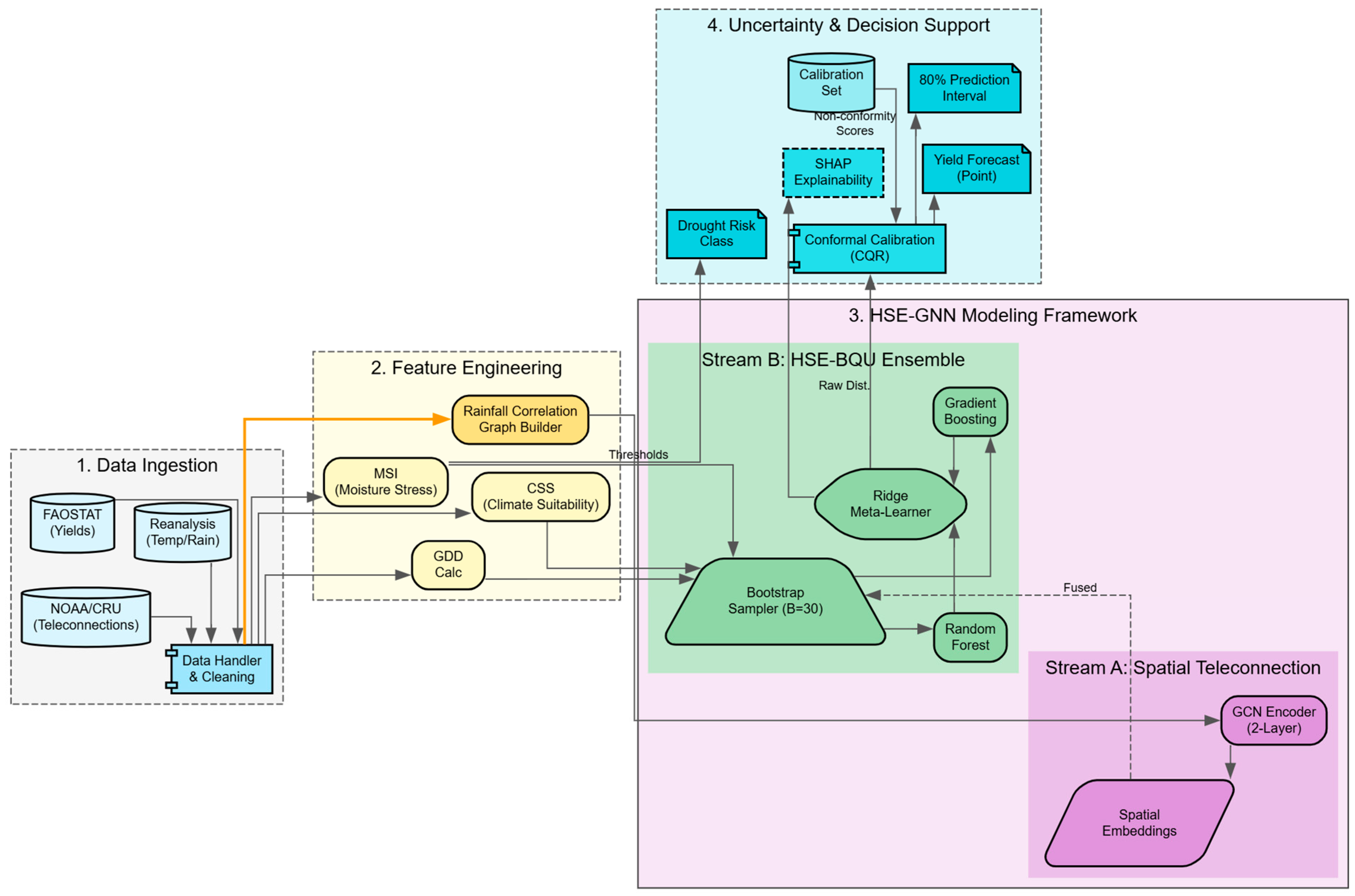
Figure 1. HSE-GNN-CP system architecture.
Information 17 00141 g001
Figure 2. Yield distribution per crop.
Information 17 00141 g002
Figure 3. Observed vs. predicted yield with conformalized intervals.
Information 17 00141 g003
Figure 4. Residual distribution.
Information 17 00141 g004
Figure 5. SHAP feature importance summary plot.
Information 17 00141 g005
Figure 6. Impact of drought severity on yield.
Information 17 00141 g006
Figure 7. Learned teleconnection matrix (rainfall correlation).
Information 17 00141 g007
Figure 8. GNN training convergence.
Information 17 00141 g008
Figure 9. GNN contribution ablation study.
Information 17 00141 g009
Table 1. Experimental configuration and hyperparameters.
CategoryComponentSpecification
HSE-BQUEnsembleBootstrap Iterations B = 30; Meta-Learner: Ridge (L2 selected via CV)
Base: Random Forest50 trees, max_depth = 12, min_samples_split = 2, max_features = √d
Base: Grad. Boost50 estimators, max_depth = 6, learning_rate = 0.1
UncertaintyConformal (CQR)Target Coverage 1 − α = 80%; Method: Higher quantile correction
GNNStructure2-Layer GCN; Hidden Dim = 64; Dropout = 0.2; Edge Threshold τ = 0.5
TrainingOptimizer: Adam (η = 0.01); Epochs: 200; Loss: MSE
ImplementationSoftwarePython 3.11, Scikit-learn 1.3, PyTorch Geometric 2.4, SHAP 0.42
HardwareIntel Core Ultra (14 cores), 16 GB RAM. Training time ≈ 15 min.
Table 2. Model performance on test set.
ModelR2RMSE (hg/ha)MAE (hg/ha)
Ridge Regression0.872186536124
RF-Standalone0.941258744231
GB-Standalone0.938560124389
HSE-BQU0.959448823487
Table 3. Uncertainty metrics (target coverage 1 − α = 80%).
MethodTarget CoverageAchieved CoverageAvg Interval Width (hg/ha)
Bootstrap (Uncalibrated)80%40.03%4790
HSE-BQU-CP (Conformalized)80%80.72%11,161
Table 4. Summary of ablation experiments.
ExperimentModel VariantR2RMSE (hg/ha)Coverage/MAE
1. CalibrationUncalibrated Bootstrap0.9594488240.03% (Cov)
HSE-BQU-CP (Proposed)0.9594488280.72% (Cov)
2. FeaturesNo Teleconnections (w/o ENSO/NAO)0.95715012-
Full Model0.95944882-
3. Ensemble SizeB = 10 Iterations0.95665124-
B = 30 Iterations (Selected)0.95874882-
B = 50 Iterations0.95874831-
4. GNN EmbeddingsBaseline + Indices0.966345343005 (MAE)
With GNN Embeddings (256-d)0.966845002993 (MAE)
Disclaimer/Publisher’s Note: The statements, opinions and data contained in all publications are solely those of the individual author(s) and contributor(s) and not of MDPI and/or the editor(s). MDPI and/or the editor(s) disclaim responsibility for any injury to people or property resulting from any ideas, methods, instructions or products referred to in the content.