Path Planning with Adaptive Autonomy Based on an Improved A^∗ Algorithm and Dynamic Programming for Mobile Robots

Abstract

Sustainable path-planning algorithms are essential for executing complex user-defined missions by mobile robots. Addressing various scenarios with a unified criterion during the design phase is often impractical due to the potential for unforeseen situations. Therefore, it is important to incorporate the concept of adaptive autonomy for path planning. This approach allows the system to autonomously select the best path-planning strategy. The technique utilizes dynamic programming with an adaptive memory size, leveraging a cellular decomposition technique to divide the map into convex cells. The path is divided into three segments: the first segment connects the starting point to the center of the starting cell, the second segment connects the center of the goal cell to the goal point, and the third segment connects the center of the starting cell to the center of the goal cell. Since each cell is convex, internal path planning simply requires a straight line between two points within a cell. Path planning uses an improved $A^{\ast }$ (I-$A^{\ast }$) algorithm, which evaluates the feasibility of a direct path to the goal from the current position during execution. When a direct path is discovered, the algorithm promptly returns and saves it in memory. The memory size is proportional to the square of the total number of cells, and it stores paths between the centers of cells. By storing and reusing previously calculated paths, this method significantly reduces redundant computation and supports long-term sustainability in mobile robot deployments. The final phase of the path-planning process involves pruning, which eliminates unnecessary waypoints. This approach obviates the need for repetitive path planning across different scenarios thanks to its compact memory size. As a result, paths can be swiftly retrieved from memory when needed, enabling efficient and prompt navigation. Simulation results indicate that this algorithm consistently outperforms other algorithms in finding the shortest path quickly.

1. Introduction

Advancements in mobile robot technologies have paved the way for their adoption in various everyday applications, such as agriculture, construction, surveillance, and transportation [1,2,3,4]. Path planning is a crucial aspect of mobile robots, serving as the backbone of their ability to autonomously navigate from one point to another for the execution of specific tasks. This is important for finding the shortest and most efficient path in the shortest amount of time [5]. For a mobile robot to navigate, it requires a map that includes the details of obstacles, as well as its current and goal locations.

Currently, path-planning algorithms are divided into three main categories: data-driven learning-based (DDLB) algorithms [1,2,6,7], memory-based (MB) algorithms [8,9], and sample-based (SB) algorithms [10]. DDLB algorithms, which leverage machine learning to optimize pathfinding, might face difficulties in generalizing across diverse environments. Specifically, an algorithm developed in one setting might not perform effectively when applied in a different environment, as DDLB heavily relies on the quality and quantity of available data. If the data is incomplete, inaccurate, or biased, it can lead to suboptimal or even unsafe path-planning decisions [1,2,11,12]. DDLB algorithms cannot learn in real time from the environment, which limits their adaptability in complex and unpredictable situations [2,13]. Some DDLB algorithms can be computationally intensive, especially when dealing with large datasets or complex environments. This can result in increased planning times, which may not be acceptable in real-time applications or resource-constrained systems [14]. DDLB models are prone to overfitting, where they learn to memorize the training data instead of capturing the underlying patterns. This can result in poor performance when deployed in real-world scenarios that differ from the training data [2,15].

MB algorithms, which rely on stored experiences and knowledge for decision-making, can store a subset of the environment’s information. This can result in incomplete representations of the environment, leading to navigation failures or suboptimal paths, especially in large or complex environments [16]. Memory constraints may require the use of compression techniques or simplified representations to accommodate the available memory. This compression can lead to information loss, reducing the accuracy of the environment representation and potentially compromising navigation performance [8]. Algorithms designed for memory-limited path planning may require additional computational resources to manage memory usage efficiently. This could result in longer planning times, limiting the feasibility of real-time navigation in dynamic environments or scenarios that require rapid decision-making [9]. The limitations of MB approaches include a risk of information loss due to compression, the need for additional planning time, and potential challenges in handling large environments.

In SB path-planning algorithms, the map is divided into a set of nodes [17] and edges [18]. Each node represents a certain part of the map, and path planning is achieved on such a set by considering how the nodes connect. In rapidly exploring random tree star (RTT*), which is a type of SB [10], the algorithm finds a path between the starting point and goal point by introducing nodes randomly and rewiring them at each step to ensure that the minimum path length reaches the goal position [17]. $A^{\ast }$, which is also a type of SB [18], is one of the best path-planning algorithms. It explores the available space in the direction of the goal by taking small steps. $A^{\ast }$ outperforms RTT* and many other path-planning algorithms [19]. The best route from the starting point to the goal is often obstacle-free [2]. $A^{\ast }$, RTT, and RTT* can find the shortest path, but they work best in open environments. However, finding a new path from the robot’s current position to the goal can be natural but very inefficient. This inefficiency occurs because the same path exploration is repeated multiple times during calculations.

This paper proposes a path-planning algorithm with the adaptive autonomy (AA) concept based on dynamic programming, I-A*, and adaptive cellular decomposition. It offers a promising solution to overcome the limitations inherent in three types of path-planning algorithms.

1.1. Short Note on Adaptive Autonomy (AA)

The first step—and one of the most critical ones—toward adaptive autonomy (AA) in different situations is finding the best system policy for handling the situation.

Adaptive autonomy (AA) is the property of an autonomous system in which the distribution of autonomy is changed dynamically to optimize overall system performance [20]. The human operator, another system, or the autonomous system itself can adjust the autonomy level [21]. Adaptive autonomy refers to the capability of autonomous agents to dynamically adjust their level of independence and control in response to changing circumstances [22,23].

1.2. Contributions

The main contributions of this paper are summarized as follows:

• A novel hybrid framework: We propose a novel path-planning framework that uniquely combines an improved A* (I-A*) algorithm with dynamic programming and adaptive cellular decomposition. This hybrid approach enables adaptive autonomy, allowing the system to select the most efficient strategy for path computation.
• Dynamic programming for computational efficiency: The algorithm leverages dynamic programming with adaptive memory to store and reuse paths between the centers of convex cells. This significantly reduces redundant calculations, especially in long-term or repetitive deployments, by allowing paths to be swiftly retrieved from memory.
• Improved A* (I-A*) algorithm for faster pathfinding: We introduce an enhanced version of the A* algorithm, termed I-A*. This algorithm accelerates the search process by continuously assessing the feasibility of a direct path to the goal, thereby minimizing the exploration of unnecessary free space.
• Path optimization: The final path is refined through a pruning process that eliminates redundant waypoints, ensuring the path is short and smooth.

In this work, we applied adaptive autonomy for path planning in various precision farming scenarios. We adopted the best policy for path planning to optimize overall system performance and effectively handle different situations.

2. Literature Review

Recent developments in path planning emphasize the adaptation and enhancement of traditional algorithms such as A* to address the challenges posed by both static and dynamic environments. Noteworthy innovations involve improving A* with methodologies tailored for dynamic settings, including replanning strategies and integration with machine learning techniques to refine heuristic accuracy. For instance, Kim and Kim describe a hybrid approach that leverages the A* algorithm for global planning while enhancing local path planning through the Analytic Hierarchy Process (AHP), highlighting the convergence of classical methods with innovative strategies to improve performance in variable conditions [24]. Additionally, research by Wang et al. explores a dynamic window method fused with an improved A* algorithm to promote more agile pathfinding for Automated Guided Vehicles (AGVs), showcasing how classical algorithms can be optimized for real-time navigational challenges [25].

In contrast, our research shifts the focus to optimizing operational efficiency in static environments, specifically enhancing the sustainability of repeated robotic tasks within consistent landscapes. This is particularly pertinent in domains like precision agriculture, where repetitive navigational tasks necessitate a more robust framework to maintain path-planning effectiveness over time. Unlike machine learning-based approaches that often require extensive datasets for training, potentially leading to issues with generalization, our adaptive autonomy (AA) framework utilizes a deterministic improved A* (I-A*) algorithm alongside dynamic programming techniques such as memoization. This structure guarantees optimal path determination between cell centers while systematically reducing computational redundancy, thereby facilitating a lightweight solution adaptable to repetitive tasks without the overhead of a training phase. These principles resonate with the findings by Zhang and Zhao, who discussed mobile robot path planning in known environments, indicating the relevance for use in static contexts like agriculture [26].

Moreover, exploring hybrid algorithms presents opportunities to integrate the strengths of diverse methodologies. For example, the integration of A* with sampling-based planners like rapidly exploring random tree (RRT) [27] combines the optimality of A* with the expansive exploratory capabilities of RRT, thus addressing efficiency while maintaining theoretical guarantees [27]. This trend underlines the pursuit of innovative crossings between classical apparatuses and new frameworks to achieve agile and effective solutions across various operational conditions. Zheng and Kuang further investigate environments characterized by uncertainty, adapting algorithmic approaches to reduce search spaces effectively, which complements the focus on static task efficiency in our work by highlighting the diverse operational contexts in which A-based solutions can evolve [28].

The efficiency of our approach is further underscored by the work of Li et al., who presented an integrated strategy combining a modified A* algorithm with the Dynamic Window Approach (DWA), achieving effective real-time path planning within the constraints of complex environments [29]. This demonstrates the adaptability of classical foundations when partnered with contemporary insights in robotic navigation—a principle reflected in our AA framework, which is constructed for optimal performance without the complexities inherent to machine learning paradigms.

3. The Proposed Path-Planning Framework with AA

The proposed AA framework for path planning incorporates dynamic programming and the I-A* algorithm. It involves multiple steps to efficiently find a path from a starting position to a goal position. A detailed description of the framework is presented below.

3.1. Adaptive Cellular Decomposition

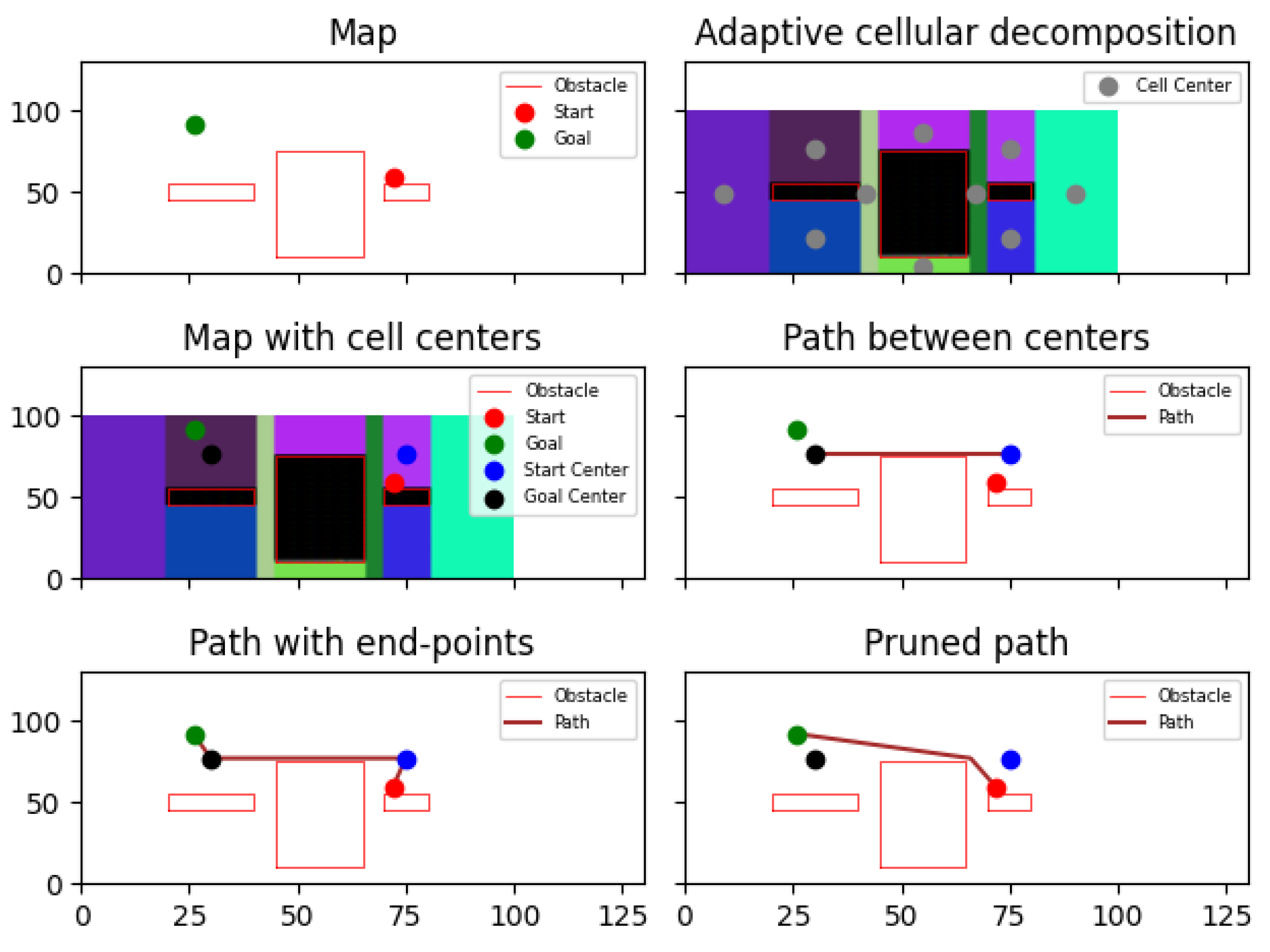
The initial step of the algorithm involves converting the map into a cellular decomposition to enable efficient path planning. The algorithm ensures that each cell generated during decomposition is convex. Convex cells simplify path-planning and navigation algorithms, as they guarantee that the shortest path between any two points within the cell does not intersect with obstacles. This property simplifies collision detection, leading to more efficient and reliable path planning. This process, visualized in Figure 1, is summarized as follows:

• Input Processing: The algorithm reads an image representing the map. Obstacles are denoted in black, while free space is represented in white. The image is then converted into a binary representation where obstacles are labeled as 0 and free space as 1.
• Connectivity Analysis: The algorithm traverses the binary image column by column, analyzing the connectivity of each column to determine contiguous areas of free space. It identifies the start and end points of each connected region within a column.
• Cell Assignment: Based on the connectivity between adjacent columns, the algorithm assigns cell IDs to the connected regions. If a region is connected to a previously identified cell, it inherits that cell’s ID; otherwise, a new cell ID is assigned.
• Cell Representation: For each identified cell, the algorithm records various properties, such as its boundaries (left, right, ceiling, floor), and calculates its center.
• Output: The algorithm saves the decomposed map, the total number of cells, and information about each cell for further analysis.

We clarify that the image is discretized into a grid. For non-rectangular obstacles, the cellular decomposition technique handles them by dividing the free space (represented by white pixels) into convex cells. This process implicitly manages obstacles of arbitrary shapes by ensuring that each generated cell is convex, simplifying internal path planning to a straight line within the cell. The binary conversion effectively identifies obstacle boundaries regardless of their shape, enabling the subsequent cellular decomposition to adapt to these complex geometries.

3.2. Memory Consumption Analysis

The claim of minimum memory usage is a cornerstone of our approach. The memory requirement is primarily dictated by the storage of paths between the centers of the decomposed cells. Let N be the total number of convex cells generated by the decomposition of a map. The memory structure is conceptually a matrix of size $N\times N$, where each entry can store a path.

The memory consumption can be quantified as

$$M_{total}=N^2\times P_{avg}\times S_{wp}$$

where N is the total number of cells, $P_{avg}$ is the average number of waypoints in a stored path, and $S_{wp}$ is the memory size of a single waypoint (e.g., 8 bytes to store two 32-bit floating-point numbers for x and y coordinates).

For example, in Map M1, which was decomposed into 10 cells ($N=10$), the memory grid has $10\times 10=100$ potential entries. Assuming that an average path between centers consists of 15 waypoints, the memory consumption would be approximately $100\times 15\times 8$ bytes = 12,000 bytes or 12 kB.

This demonstrates a significant advantage: instead of storing path data for a potentially infinite number of start/goal scenarios, we only need to store a finite number of inter-cell paths. The memory growth is polynomial ($O\left(N^2\right)$) with respect to the number of cells, not the map’s resolution or complexity, ensuring scalability.

It is important to note that while many of the obstacles in our test maps are composed of straight edges, the adaptive cellular decomposition technique itself is not constrained to such environments. The method processes the map based on free-space connectivity, column by column, allowing it to generate convex cells around obstacles of arbitrary shapes. The inclusion of concave obstacles in Maps M2, M6, and M7 was specifically intended to validate this capability.

3.3. Improved $A^{\ast }$ Algorithm

The $A^{\ast }$ search algorithm, which is a popular pathfinding algorithm, used to find the shortest path between a start node and an end node in a graph or grid. The algorithm begins by initializing the open and closed sets. The F-cost, which guides the search, is computed as the sum of the G-cost (actual cost from the start) and the H-cost (heuristic to the goal). Starting from the initial node, the algorithm repeatedly selects the node with the lowest F-cost, explores its neighbors, updates their costs if a better path is found, and continues until the goal is reached or no path exists. If the goal is reached, the shortest path is returned. The $A^{\ast }$ algorithm combines information from both the path cost and heuristic cost to reach a node ($g_{cost}$) and a heuristic estimate of the remaining cost to reach the goal ($h_{cost}$). This combination allows $A^{\ast }$ to make informed decisions about which nodes to explore next, leading to an optimal path in terms of both cost and efficiency.

In the $A^{\ast }$ algorithm, the map is converted into a grid, and exploration of the path in the direction of the goal point is guided by the heuristic cost value $f_{cost}=g_{cost}+h_{cost}$, where $g_{cost}$ is the displacement between the current node and the starting node, and $h_{cost}$ is the distance between the current node and the goal node. In the $A^{\ast }$ path-planning algorithm, the map is defined by M, the free space is defined by $M_{free}$, and the obstacles are defined by $M_{obs}$. The $A^{\ast }$ algorithm relies on its cost function for path planning. The path calculated by $A^{\ast }$ consists of adjacent cells of the grid, which makes it long and saw-tooth due to the discrete grid representation, suboptimal heuristic choices, and tie-breaking methods favoring frequent turns [30].

I-$A^{\ast }$ Algorithm

This section discusses the modifications made to the $A^{\ast }$ algorithm to enhance its efficiency in terms of execution time, path length, and the number of waypoints. The exploration of free space begins from the starting point and proceeds toward the goal point by taking small steps of length.

After each step, the I-A* algorithm assesses the environment by examining the obstacles between the current point and the goal position. This assessment allows the algorithm to avoid unnecessary free-space exploration not required to reach the goal position. As a result, the algorithm reaches the goal position by navigating around obstacles, minimizing the exploration of unwanted free space. In contrast, the original $A^{\ast }$ algorithm takes continuous small steps without considering the map’s overall situation, leading to the exploration of unnecessary free space and additional steps.

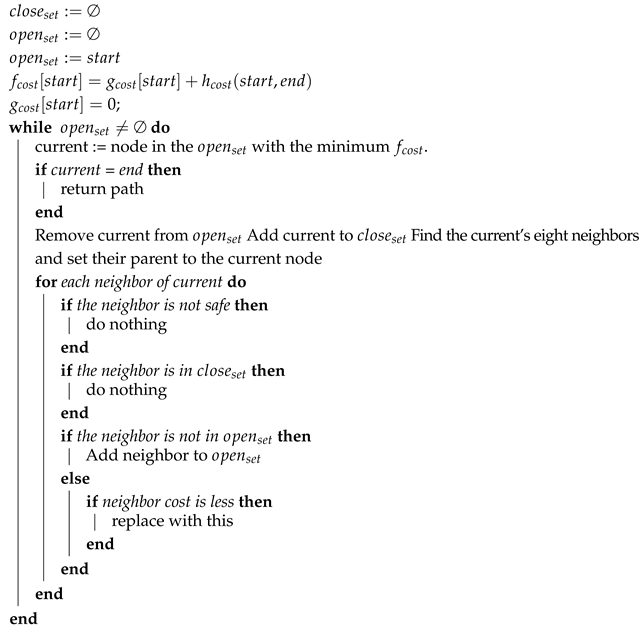
Once the goal point is reached, a step-wise path is generated by backtracking through the connected grid cells from the goal point to the starting point. This process requires fewer steps compared to the original $A^{\ast }$ algorithm, contributing to improved efficiency in terms of execution time, the number of waypoints, and the length of the path. The pseudocodes for the original $A^{\ast }$ algorithm and the improved $A^{\ast }$ algorithm are presented in Algorithms 1 and 2, respectively. To contextualize our improvements, we first present the pseudocode for the standard A* algorithm, which serves as a baseline for our I-A* variant. Although the final path may contain additional waypoints, these can be eliminated through post-pruning steps [31], as demonstrated in Figure 2.

Algorithm 1:  $A^{\ast }(start,end,obstacles)$

Algorithm 2: I-A*

3.4. Path Generation Using Dynamic Programming

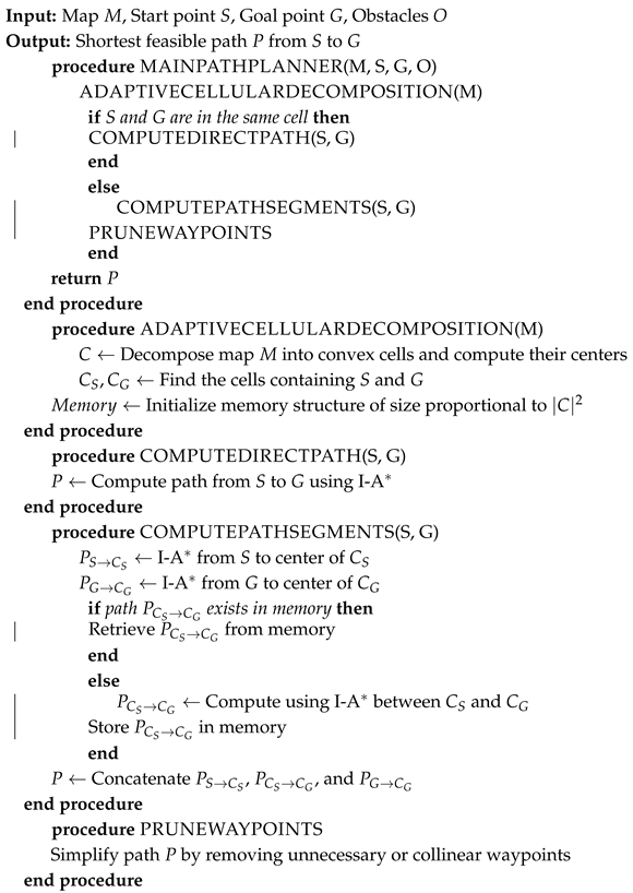
The proposed Algorithm 3 employs a strategic approach that introduces adaptive autonomy in dynamic programming and the A* algorithm to solve a path-planning problem on a map with obstacles. The map is divided into convex cells, which simplifies the path-planning process because the path within a cell is straight.

Algorithm 3: AA using dynamic programming and I-A*

In the context of this paper, the application of dynamic programming is realized through memoization. The complex problem of global path planning is decomposed into a set of smaller, recurring subproblems—namely, calculating the optimal path between the centers of any two cells. Our algorithm computes the path for each subproblem once and stores the result in memory. For all subsequent requests involving the same subproblem, the solution is retrieved directly from this memory cache. This approach of storing and reusing solutions to overlapping subproblems is a fundamental characteristic of dynamic programming, significantly reducing computational overhead and enabling swift path retrieval.

A breakdown of the various components and procedures in the proposed algorithm is presented in the next section.

• Components

• Map (M): This represents the terrain or environment, including the starting point S, the goal point G, and the list of obstacles O.
• Convex Cells (C): The map is decomposed into these cells, each having a center, simplifying the navigation by breaking down the larger problem into smaller, manageable units.
• Cell Centers ($C_S$ and $C_G$): These are the specific centers of the cells containing the starting point and the goal point, respectively.

• Procedures

• Adaptive Cellular Decomposition

The following procedures handle the initial setup:

• Decompose the Map: The map is divided into convex cells, and the center of each cell is computed.
• Identify Relevant Cells: Identifies the specific cells ($C_S$ for start, $C_G$ for goal) that contain the starting and goal points.
• Initialize Memory: Initializes memory storage to keep paths between centers, sized based on the number of cells squared, allowing for efficient path retrieval and reduced computation.

• If Starting Point and Goal Point in Same Cell

This conditional procedure handles the scenario where the start and goal points are within the same cell:

• Direct Path Computation: Directly computes the path from the starting point to the goal point using $I-A^{\ast }$ without the need to transition between multiple cell centers, simplifying the process and reducing computation.

• If Starting Point and Goal Point Are Not in Same Cell

This overarching procedure encompasses several steps for when the start and goal points are not in the same cell:

• Compute Path Segments

• Paths to Cell Centers: Computes paths from the start point to its cell center ($P_{S_{C_S}}$) and from the goal point to its cell center ($P_{G_{C_G}}$) using $I-A^{\ast }$.
• Path Between Centers:
  • Checks whether the path between the centers ($P_{C_S{C}_G}$) has been previously calculated and is available in memory.
  • If not, computes this path using $I-A^{\ast }$ and saves it in memory.
• Combine Paths: Integrates the computed paths (from start to start center, between centers, from goal center to goal) into a single path ($P_{S{C}_S{C}_S{C}_{G}G{C}_G}$).

• PruneWaypoints

• Pruning: Removes unnecessary waypoints from the combined path to ensure it is the most efficient path, resulting in the final path (P) that contains only necessary waypoints.

However, the path obtained so far is not the shortest, as can be seen in Figure 2. To make it the shortest path with fewer waypoints, path pruning is performed as a post-processing step.

4. Experimental Setup

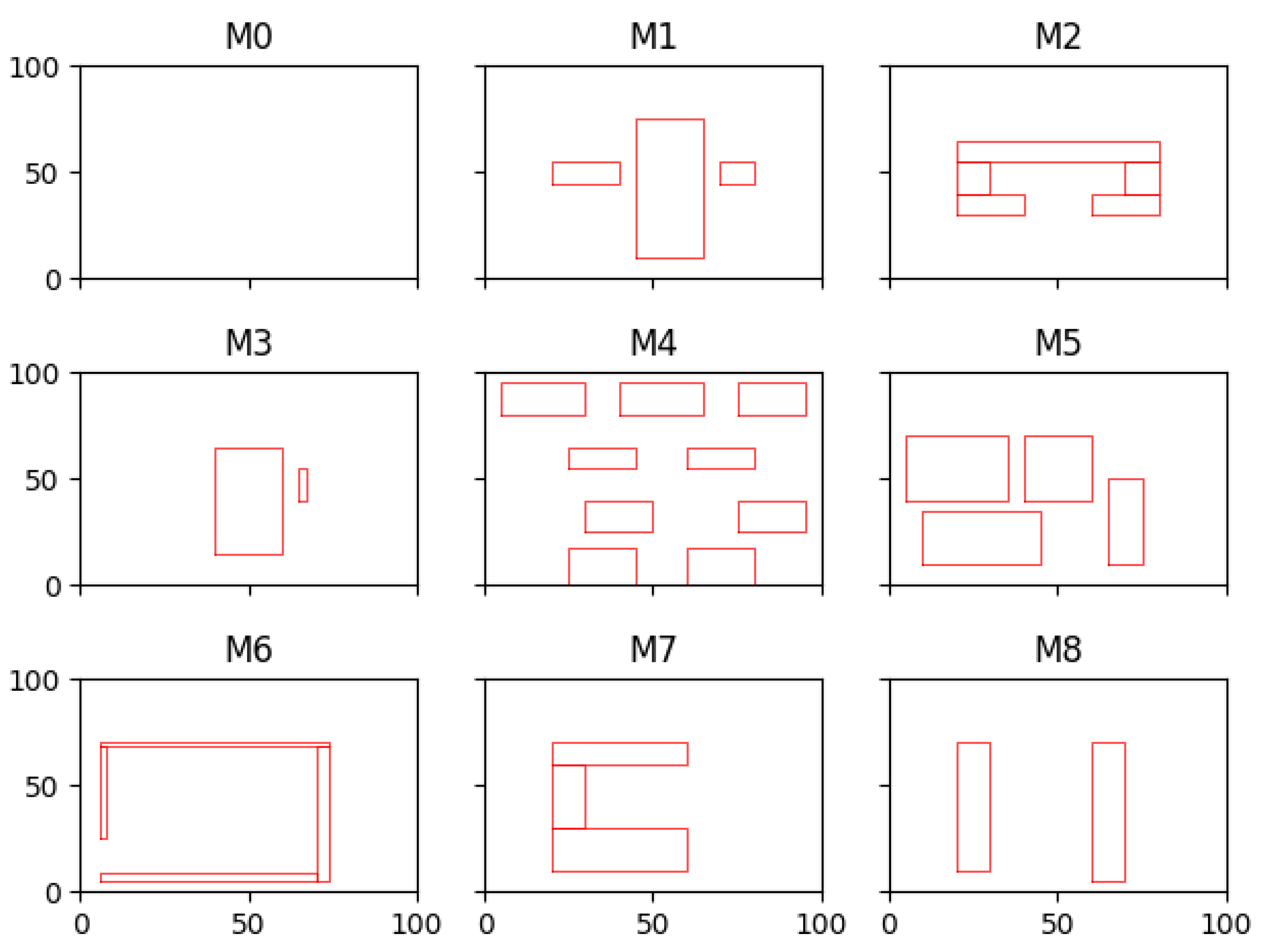
For the data and experimentation, we used nine different maps (M0, M1, M2, M3, M4, M5, M6, M7, and M8) with 3000 scenarios, as summarized in

Table 1. Map parameters.

Map	No. of Obstacles	Area of Obstacles (%)
M0	0	0
M1	3	29
M2	1	17
M3	2	17
M4	9	21
M5	4	43
M6	1	7
M7	1	24
M8	2	20

and shown in Figure 3.

To ensure a comprehensive and unbiased evaluation of the algorithms, a total of 3000 test scenarios were systematically generated across the nine maps. For each scenario, the start and goal points were chosen by randomly sampling coordinates within the map’s designated free space (represented as white areas in the map images). This process guaranteed that all generated start and goal locations were valid (i.e., not within an obstacle) and provided a diverse set of pathfinding challenges, ranging from simple, direct paths to complex routes requiring significant navigation around obstacles.

Map M0 is the simplest scenario, as it contains no obstacles. M1 contains one obstacle. M3 and M9 contain two obstacles, each of a different size. M4 contains four obstacles with low density. M5 contains four obstacles with high density. However, to check the robustness of the algorithm in the proposed approach, concave obstacles with different complexity levels were used in Maps M2, M6, and M7. Maps M1, M2, M3, and M4 were inspired by previous approaches [10,32,33]. A simulation setup was developed in Python 3.12 using PyTorch 2.4. The operating system was 64-bit Windows 10 with an Intel(R) Core(TM) i5-9300H CPU @ 2.40 GHz and 8 GB of RAM. (Intel Corporation, Santa Clara, CA, USA).

To ensure a fair and direct comparison, all algorithms were executed on the same hardware platform under identical conditions. The A* and RRT algorithms used for benchmarking are based on standard, widely accepted implementations, without any specific optimizations, to provide a consistent baseline for evaluating the performance gains of our proposed I-A* and AA frameworks.

Map Parameters

Table 1 summarizes the various maps along with their corresponding parameters. Each row in the table represents a unique map, while the columns provide details about the number of obstacles present on each map and the percentage of area occupied by these obstacles.

The maps are summarized as follows:

• Map M0: Contains no obstacles, with 0% of the area occupied by obstacles.
• Map M1: Contains three obstacles, which occupy 29% of the total area.
• Map M2: Contains one obstacle, which covers 17% of the total area.
• Map M3: Contains two obstacles, covering 17% of the total area.
• Map M4: Contains nine obstacles, occupying 21% of the total area.
• Map M5: Contains four obstacles, covering 43% of the total area.
• Map M6: Contains one obstacle, which occupies 7% of the total area.
• Map M7: Contains one obstacle, covering 24% of the total area.
• Map M8: Contains two obstacles, occupying 20% of the total area.

5. Results and Analysis

Table 2. Comparison of accuracy between deep learning-based path planning and AA with I-A*.

Algorithm	Scenario	Accuracy
Deep learning-based path planning [2]	3000	61%
AA with I-A*	3000	100%

presents a comparison of the accuracy between two path-planning algorithms: deep learning-based path planning and AA with I-A*.

Deep learning-based path planning: For comparison, we benchmarked our approach against a deep learning-based path-planning algorithm from our prior work, in which a Convolutional Recurrent Neural Network (CRNN) was used to process the map as an image. The model’s architecture consists of convolutional layers to extract spatial features from the map, followed by recurrent layers to capture sequential information, and finally, a dense layer to predict the path. The model was trained on a dataset of 2000 scenarios per map, learning to generate a feasible path from a given start and goal point. The 61% accuracy reported reflects its performance on a test set of 3000 previously unseen scenarios, where a ‘successful’ plan was both collision-free and reached the goal [2].

AA with I-A*: Our approach demonstrated superior performance, with a perfect accuracy of 100% on the same dataset.

Overall, AA with the I-A* algorithm outperformed the deep learning-based path-planning algorithm, achieving higher accuracy and reliability in generating paths.

5.1. Time and Space Complexity Analysis

The proposed framework integrates adaptive cellular decomposition, an improved A* (I-A*) algorithm, and dynamic programming. The following is a detailed breakdown of its computational complexity:

• Adaptive Cellular Decomposition: This step converts the binary map of size $m\times n$ into a set of convex cells by scanning columns and analyzing connectivity.

  -

  Time Complexity: $O\left(mn\right)$, since each pixel is visited once during decomposition.

  -

  Space Complexity: $O(mn+N)$, where N is the number of convex cells.

• Path Storage with Memoization (Dynamic Programming): Precomputes and stores paths between cell centers to avoid redundant computation.

  -

  Time Complexity: $O(N^2·T)$ in the worst case, where T is the time to compute a path using I-A*. Subsequent lookups are completed in $O\left(1\right)$ time.

  -

  Space Complexity: $O(N^2·P_{\mathrm{avg}}·S_{\mathrm{wp}})$, where $P_{\mathrm{avg}}$ is the average number of waypoints per path and $S_{\mathrm{wp}}$ is the memory per waypoint.

• Improved A* (I-A*) Algorithm: Enhances the standard A* algorithm by avoiding unnecessary exploration when a direct path is visible, significantly reducing computational cost in many cases:

  -

  Time Complexity: $O\left(b^{d^{\prime }}\right)$, where b is the branching factor and $d^{\prime }\ll d$ due to early termination and selective expansion.

  -

  Space Complexity: $O\left(k\right)$, where k is the number of explored nodes, which is significantly smaller than $mn$ in sparse environments.

• Path Pruning: This post-processing step simplifies the path by removing collinear or unnecessary waypoints:

  -

  Time Complexity: $O\left(P\right)$, where P is the total number of waypoints in the raw path.

  -

  Space Complexity: $O\left(P\right)$, as it only requires storage proportional to the path length.

Overall, the algorithm is designed to scale efficiently with map size and complexity. The most computationally expensive step, intercell path storage, grows with the square of the number of cells, not the map resolution, offering a good trade-off between performance and memory.

5.2. Time Efficiency Analysis

Table 3. Time efficiency in ms.

Map	${\mathit{A}}^{\ast }$	I-${\mathit{A}}^{\ast }$	RRT
M0	241	0.11	1380
M1	2485	1612	13,343
M2	5455	3500	31,203
M3	3420	1603	27,031
M4	8606	5722	38,191
M5	2910	2011	25,328
M6	9966	8315	209,048
M7	6487	5323	32,969
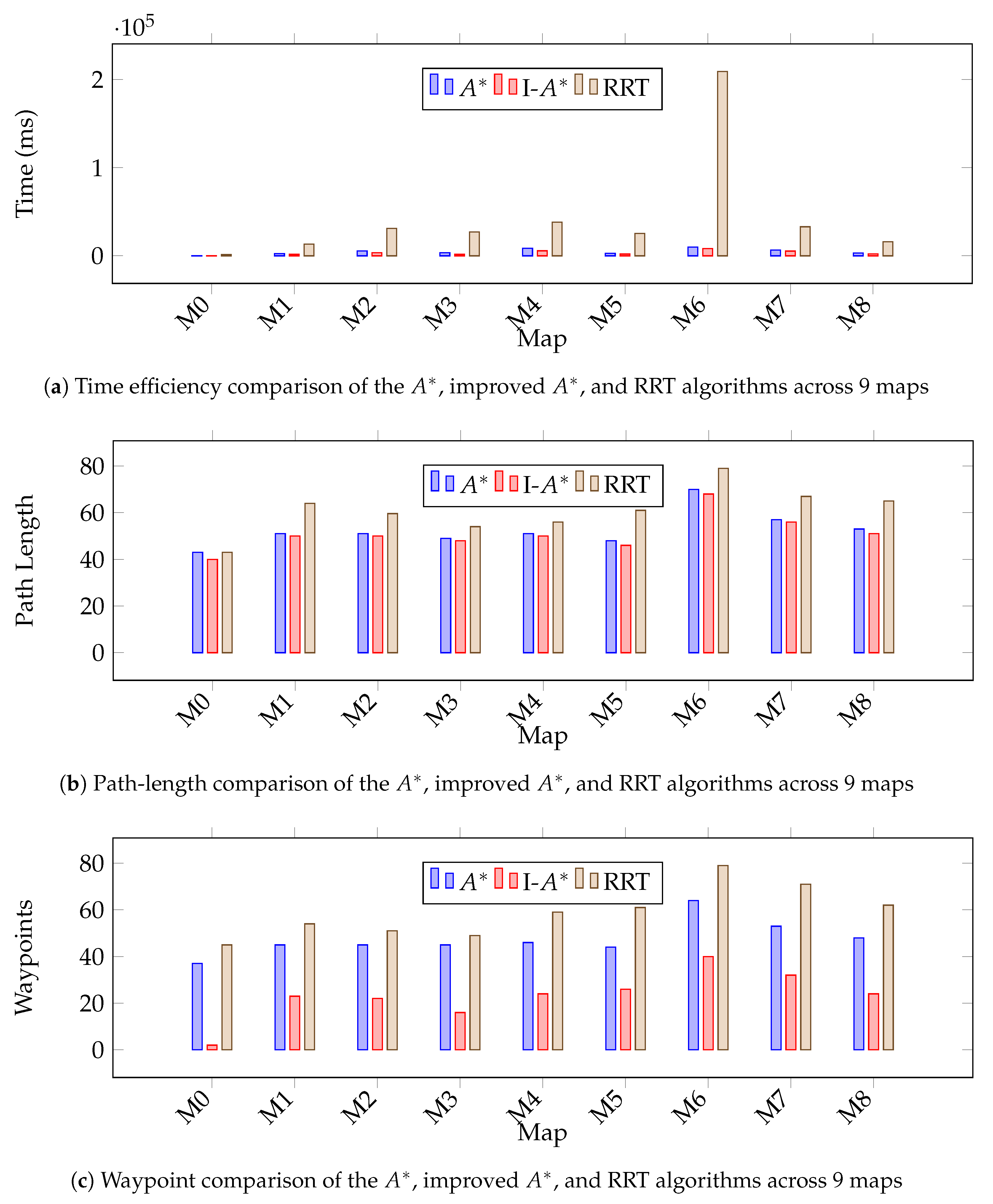
M8	3064	2063	15,914

presents the time taken in milliseconds to compute a feasible path using three different path-planning algorithms: A*, improved A* (I-A*), and rapidly exploring random tree (RRT) [27]. Each row in the table corresponds to a different map, and the columns show the execution time required by each algorithm to complete the path-planning task on that map. This time metric reflects the computational efficiency of each method in generating a valid, collision-free path from the start to the goal. Lower values generally indicate higher time efficiency.

The time efficiency is calculated as the difference between the time when the function is called and the time when the path computation is complete, as defined in Equation (1).

$$\mathrm{Time}\mathrm{Efficiency}=t_{\mathrm{end}}-t_{\mathrm{start}}$$

(1)

Below is a summary of the table:

• Map M0: The $A^{\ast }$ algorithm took 241 ms, the I-A* algorithm took 0.11 ms, and the RRT algorithm took 1380 ms to complete the path-planning task.
• Map M1: The $A^{\ast }$ algorithm took 2485 ms, the I-A* algorithm took 1612 ms, and the RRT algorithm took 13,343 ms for this map.
• Map M2: The $A^{\ast }$ algorithm took 5455 ms, the I-A* algorithm took 3500 ms, and the RRT algorithm took 31,203 ms.
• Map M3: The $A^{\ast }$ algorithm took 3420 ms, the I-A* algorithm took 1603 ms, and the RRT algorithm took 27,031 ms.
• Map M4: The $A^{\ast }$ algorithm took 8606 ms, the I-A* algorithm took 5722 ms, and the RRT algorithm took 38,191 ms for this map.
• Map M5: The $A^{\ast }$ algorithm took 2910 ms, the I-A* algorithm took 2011 ms, and the RRT algorithm took 25,328 ms.
• Map M6: The $A^{\ast }$ algorithm took 9966 ms, the I-A* algorithm took 8315 ms, and the RRT algorithm took 209,048 ms.
• Map M7: The $A^{\ast }$ algorithm took 6487 ms, the I-A* algorithm took 5323 ms, and the RRT algorithm took 32,969 ms for this map.
• Map M8: The $A^{\ast }$ algorithm took 3064 ms, the I-A* algorithm took 2063 ms, and the RRT algorithm took 15,914 ms.

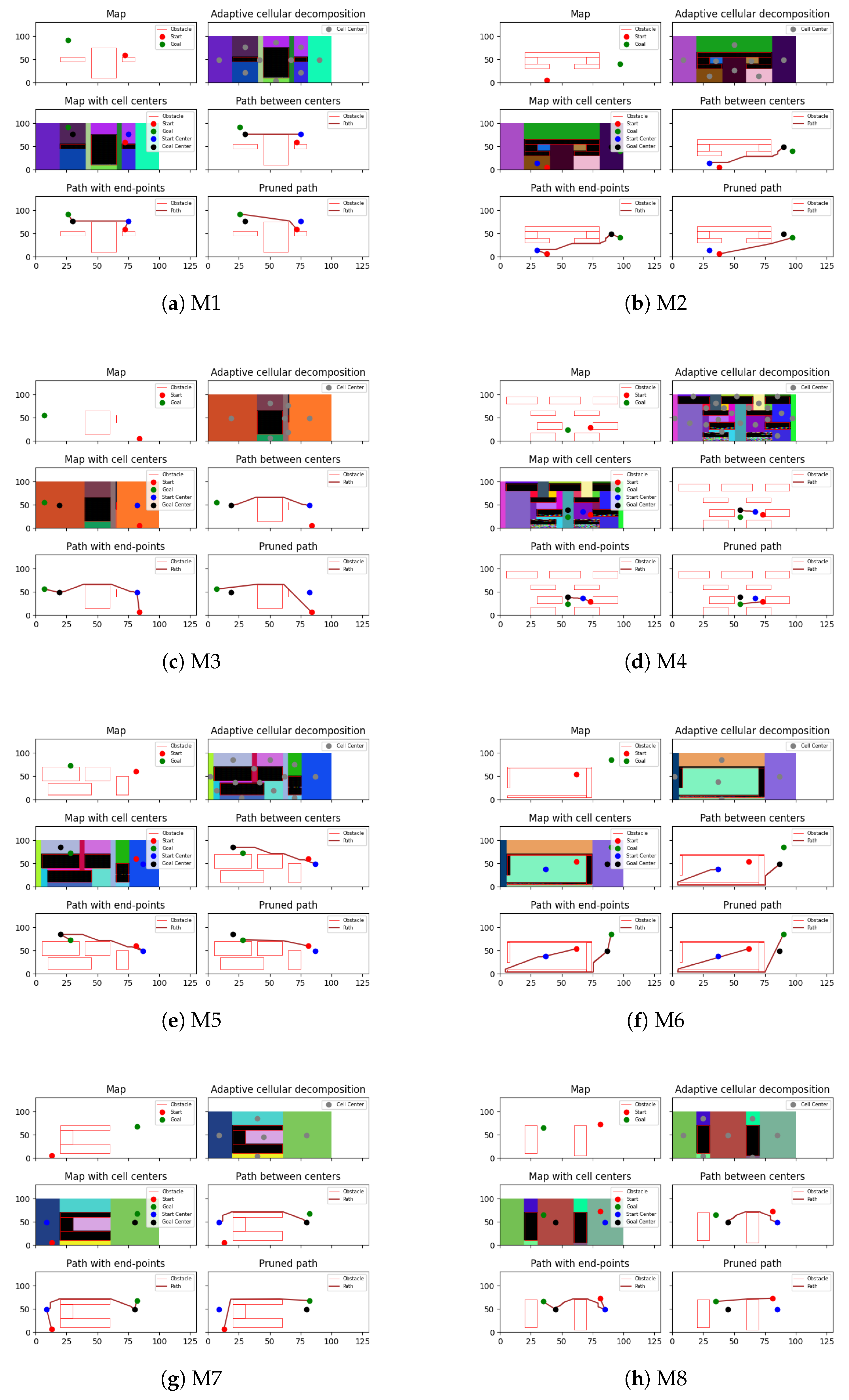
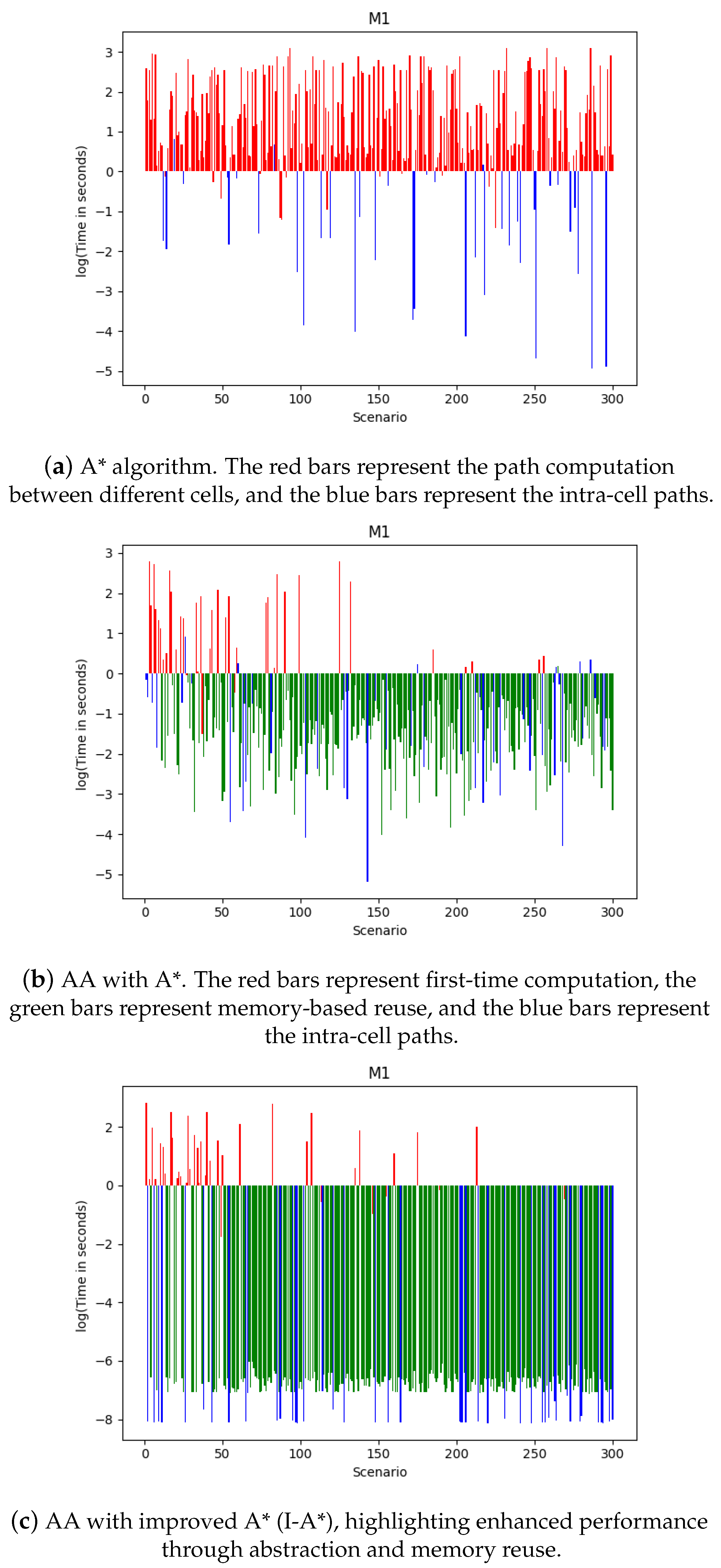
The proposed methodology was tested on eight different maps to show its effectiveness, as shown in Figure 4a–c. Each map includes the available free space, obstacles, a starting point, and a goal point. Adaptive cellular decomposition divides the space into distinct cells, each visualized with a different color, with their centers marked in gray. Each map shows a starting point with the starting point’s cell center and a goal point with the goal point’s cell center. The path between centers represents the shortest path between these centers and is also saved in memory. The path with endpoints shows the combined path between the cell centers and their corresponding start and end points. The pruned path represents the path with extra waypoints removed; hence, it is the shortest path.

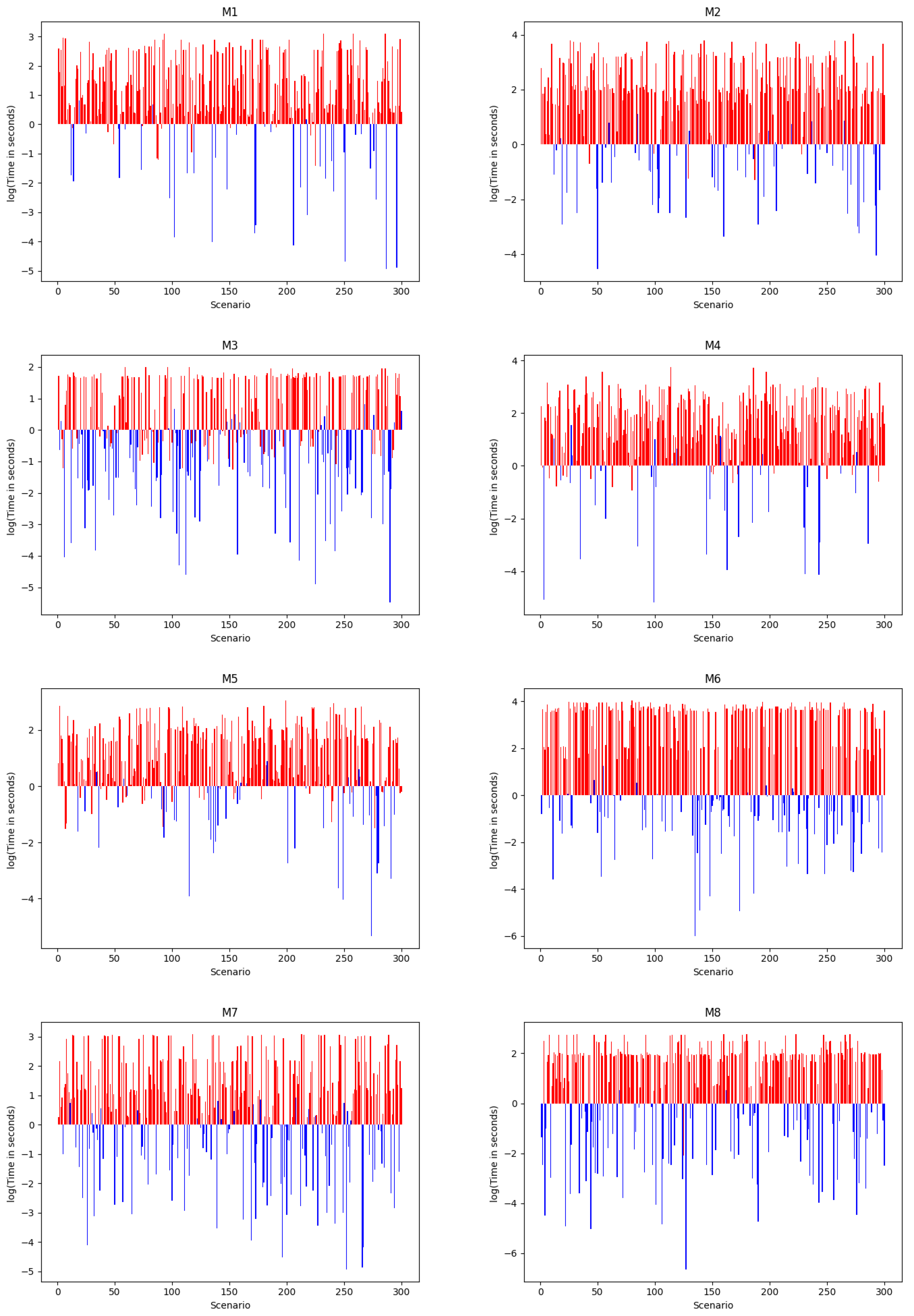
The execution time comparison charts in Figure 4a–c are presented on a logarithmic scale and illustrate the efficiency of different path-planning methods for the M1 scenario.

The analysis below summarizes the proportions of colored bars and the mean execution times shown in the above figure.

Percentage of red bars:

• $A^{\ast }$: Approximately 85% of the bars are red, indicating that a significant proportion of time was spent calculating paths between different cells.
• AA with $A^{\ast }$: Around 15% of the bars are red, suggesting a smaller fraction of time was dedicated to initial path calculations and memory storage.
• AA with I-A*: Around 15% of the bars are red, indicating similar behavior to AA with $A^{\ast }$.

Percentage of blue bars:

• $A^{\ast }$: Around 12% of the bars are blue, representing the time taken to calculate the shortest path within the same cell using the $A^{\ast }$ algorithm.
• AA with $A^{\ast }$: Approximately 13% of the bars are blue, indicating that a similar proportion of time was spent on intra-cell path calculations.
• AA with I-A*: Around 12% of the bars are blue, again indicating similar behavior to AA with $A^{\ast }$.

Percentage of green bars:

• $A^{\ast }$: Not applicable, as $A^{\ast }$ does not involve path calculations between different cells using memory.
• AA with $A^{\ast }$: Around 87% of the bars are green, representing the time spent calculating paths between different cells using stored memory.
• AA with I-A*: Approximately 88% of the bars are green, indicating similar behavior to AA with $A^{\ast }$.

Mean execution time (logarithmic scale):

• Red bars:

  -

  $A^{\ast }$: The mean execution time was around 1.5, indicating the average time spent on inter-cell path calculations.

  -

  AA with $A^{\ast }$: The mean execution time was around 1.4, suggesting a slightly lower average time spent on initial path calculations and memory storage compared to $A^{\ast }$.

  -

  AA with I-A*: The mean execution time was around 1.3, indicating a further improvement in the average time spent on initial path calculations and memory storage compared to both $A^{\ast }$ and AA with $A^{\ast }$.

• Blue bars:

  -

  $A^{\ast }$: The mean execution time was around −2.4, representing the average time taken for intra-cell path calculations.

  -

  AA with $A^{\ast }$: The mean execution time was around −2.3, indicating a similar average time for intra-cell path calculations to $A^{\ast }$.

  -

  AA with I-A*: The mean execution time was around −7, suggesting a significant improvement compared to both $A^{\ast }$ and AA with $A^{\ast }$.

• Green bars:

  -

  $A^{\ast }$: Not applicable, as $A^{\ast }$ does not involve path calculations between different cells using memory.

  -

  AA with $A^{\ast }$: The mean execution time was around −1.5, representing the average time for path calculations between different cells using stored memory.

  -

  AA with I-A*: The mean execution time was around −6, indicating a substantial improvement compared to AA with $A^{\ast }$.

Standard deviation (logarithmic scale):

• Red bars:

  -

  $A^{\ast }$: The standard deviation was around 4.6, indicating the variability in the time spent on inter-cell path calculations.

  -

  AA with $A^{\ast }$: The standard deviation was around 3.9, suggesting slightly lower variability compared to $A^{\ast }$.

  -

  AA with I-A${\mathrm{I}-\mathrm{A}}^{\ast }$: The standard deviation was around 3.9, indicating similar variability to AA with $A^{\ast }$.

• Blue bars:

  -

  $A^{\ast }$: The standard deviation was around 4, representing variability in the time spent on intra-cell path calculations.

  -

  AA with $A^{\ast }$: The standard deviation was around 3, indicating slightly lower variability compared to $A^{\ast }$.

  -

  AA with ${\mathrm{I}-\mathrm{A}}^{\ast }$: The standard deviation was negligible (around 0), suggesting significantly lower variability than both $A^{\ast }$ and AA with $A^{\ast }$.

• Green bars:

  -

  $A^{\ast }$: Not applicable, as $A^{\ast }$ does not involve path calculations between different cells using memory.

  -

  AA with $A^{\ast }$: The standard deviation was around 4, indicating variability in the time spent on path calculations between different cells using stored memory.

  -

  AA with ${\mathrm{I}-\mathrm{A}}^{\ast }$: The standard deviation was negligible (around 0), suggesting significantly reduced variability compared to AA with $A^{\ast }$.

The following discussion highlights the improvements introduced by incorporating AA into the $A^{\ast }$ algorithm:

• $A^{\ast }$ Algorithm:

  (a)

  The $A^{\ast }$ algorithm took a significant amount of time to calculate the path in these scenarios.

  (b)

  It was relatively efficient when calculating the path within the same cell, as indicated by the fewer blue bars.

  (c)

  The average execution time on the logarithmic scale was moderate but not exceptionally fast.

  (d)

  The high standard deviation in the execution time suggests that the algorithm’s performance varied significantly across different scenarios.

• AA with $A^{\ast }$ Algorithm:

  (a)

  This algorithm was significantly faster in calculating the path compared to $A^{\ast }$.

  (b)

  It efficiently computed the path within the same cell.

  (c)

  The average execution time on the logarithmic scale was negative, indicating that it was faster than the reference algorithm.

  (d)

  The moderate standard deviation in the execution times suggests some variability in performance across different scenarios.

• AA with ${\mathrm{I}-\mathrm{A}}^{\ast }$ Algorithm:

  (a)

  This algorithm was significantly faster in calculating the path compared to the reference algorithm.

  (b)

  The average execution time on the logarithmic scale was negative, indicating that it was significantly faster.

  (c)

  The low standard deviation in the execution time suggests consistent and stable performance across scenarios.

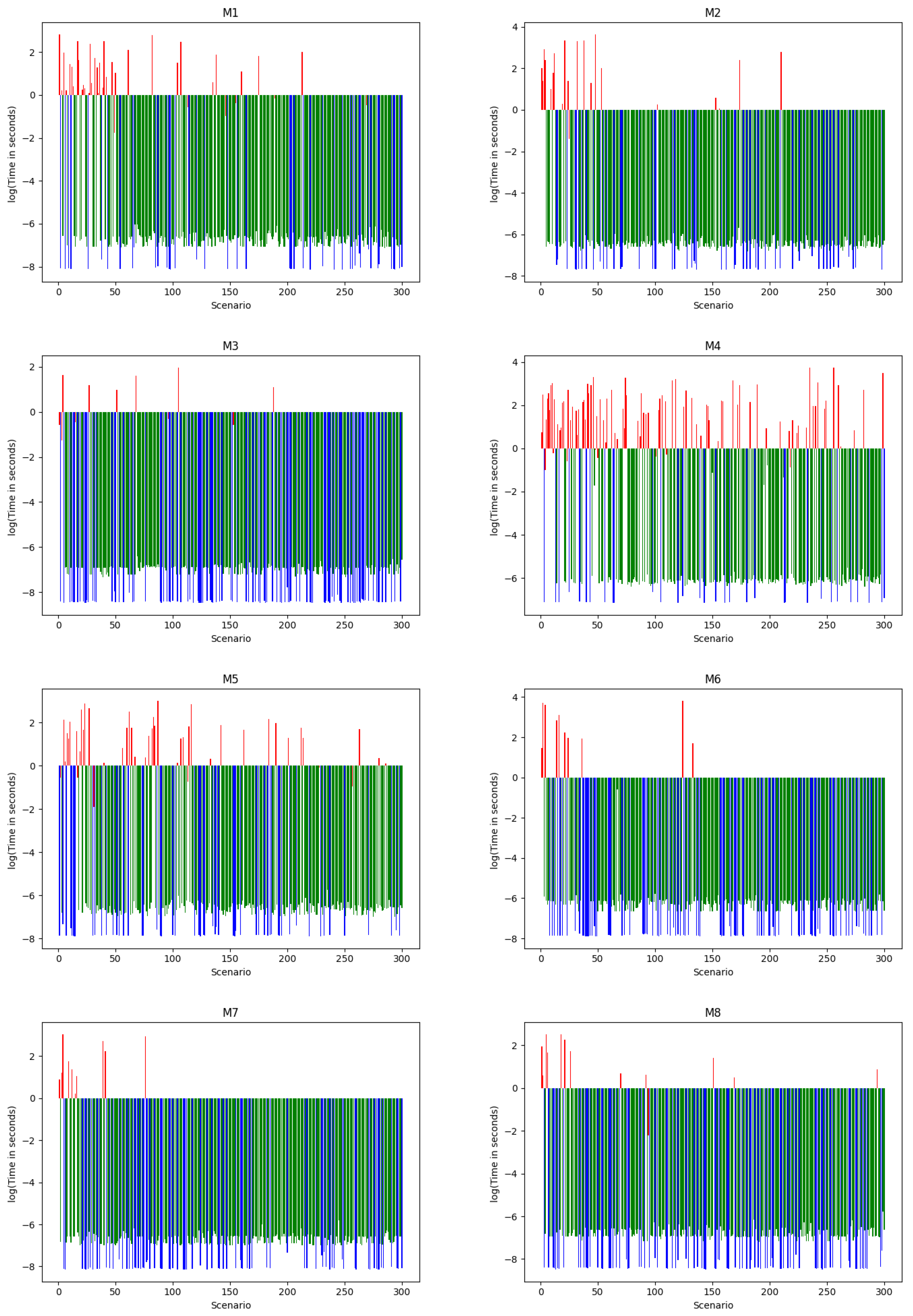
In summary, both AA algorithms ($A^{\ast }$ and improved $A^{\ast }$) demonstrated remarkable speed advantages over the reference algorithm ($A^{\ast }$) in calculating paths in the given 300 scenarios on Map M6. Additional experimental results supporting the proposed approach are provided in the Appendix. Specifically, Figure A1 illustrates the path-planning outcomes across various maps using AA, while Figure A2 and Figure A3 present execution time comparisons for the A${\mathrm{A}}^{\ast }$ algorithms, respectively.

5.3. Path-Length Comparison

Table 4. Path lengths.

Map	${\mathit{A}}^{\ast }$	I-${\mathit{A}}^{\ast }$	RRT
M0	43	40	43
M1	51	50	64
M2	51	50	59.6
M3	49	48	54
M4	51	50	56
M5	48	46	61
M6	70	68	79
M7	57	56	67
M8	53	51	65

provides a comparison of the path lengths generated by the three algorithms ($A^{\ast }$, ${\mathrm{I}-\mathrm{A}}^{\ast }$, and RRT) across different maps. Each row represents a different map, and the columns show the path length obtained by each algorithm for that map. Smaller values indicate shorter path lengths.

RRT Settings: Step size = 10 units; goal bias = 0.1; goal threshold = 5 units; max. iterations = 2000.

The results in the table can be summarized as follows:

• Map M0: The path length for this map was 43 units for the $A^{\ast }$, ${\mathrm{I}-\mathrm{A}}^{\ast }$, and RRT algorithms.
• Map M1: The $A^{\ast }$ algorithm generated a path length of 51 units, the ${\mathrm{I}-\mathrm{A}}^{\ast }$ algorithm produced a path length of 50 units, and the RRT algorithm generated a path length of 64 units.
• Map M2: The path length obtained by the $A^{\ast }$ and ${\mathrm{I}-\mathrm{A}}^{\ast }$ algorithms was 51 units, while the RRT algorithm generated a path length of 59.6 units.
• Map M3: The $A^{\ast }$ algorithm generated a path length of 49 units, the ${\mathrm{I}-\mathrm{A}}^{\ast }$ algorithm generated a path length of 48 units, and the RRT algorithm produced a path length of 54 units.
• Map M4: The path length obtained by the $A^{\ast }$ and ${\mathrm{I}-\mathrm{A}}^{\ast }$ algorithms was 51 units, while the RRT algorithm generated a path length of 56 units.
• Map M5: The $A^{\ast }$ algorithm generated a path length of 48 units, the ${\mathrm{I}-\mathrm{A}}^{\ast }$ algorithm generated a path length of 46 units, and the RRT algorithm produced a path length of 61 units.
• Map M6: The path length obtained by the $A^{\ast }$ and ${\mathrm{I}-\mathrm{A}}^{\ast }$ algorithms was 70 units, while the RRT algorithm generated a path length of 79 units.
• Map M7: The $A^{\ast }$ algorithm generated a path length of 57 units, the ${\mathrm{I}-\mathrm{A}}^{\ast }$ algorithm generated a path length of 56 units, and the RRT algorithm produced a path length of 67 units.
• Map M8: The path length obtained by the $A^{\ast }$ and ${\mathrm{I}-\mathrm{A}}^{\ast }$ algorithms was 53 units, while the RRT algorithm generated a path length of 65 units.

5.4. Comparison of Path-Planning Algorithms

This section compares three path-planning algorithms (A*, improved A* (I-A*), and RRT) on nine maps (M0 to M8) using three key metrics:

• Time Efficiency (ms): I-A* outperformed both A* and RRT, providing faster execution times on all maps.
• Path Length: I-A* produced the shortest paths, while RRT often generated the longest and most irregular ones.
• Waypoints: I-A* used significantly fewer waypoints, suggesting a smoother trajectory. RRT required the most.

As shown in Figure 5a–c, the improved $A^{\ast }$ algorithm demonstrated superior time efficiency and generated shorter paths than both $A^{\ast }$ and RRT across most maps.

6. Conclusions and Future Work

In this paper, we have introduced a path-planning algorithm with adaptive autonomy (AA). The algorithm incorporates an improved form of $A^{\ast }$, referred to as I-$A^{\ast }$, which assesses the feasibility of a direct path to the goal from the current position during execution. The execution time comparison chart highlights the effectiveness of AA in reducing the number of path calculations and improving efficiency compared to the traditional $A^{\ast }$ algorithm. Both AA with $A^{\ast }$ and AA with I-A* demonstrate significant reductions in path calculations between different cells. Moreover, the use of memory for path calculations leads to additional efficiency gains. The average execution times and standard deviations indicate the improved performance and consistency achieved by the AA approaches, with AA using dynamic programming and I-A* showing the highest level of efficiency.

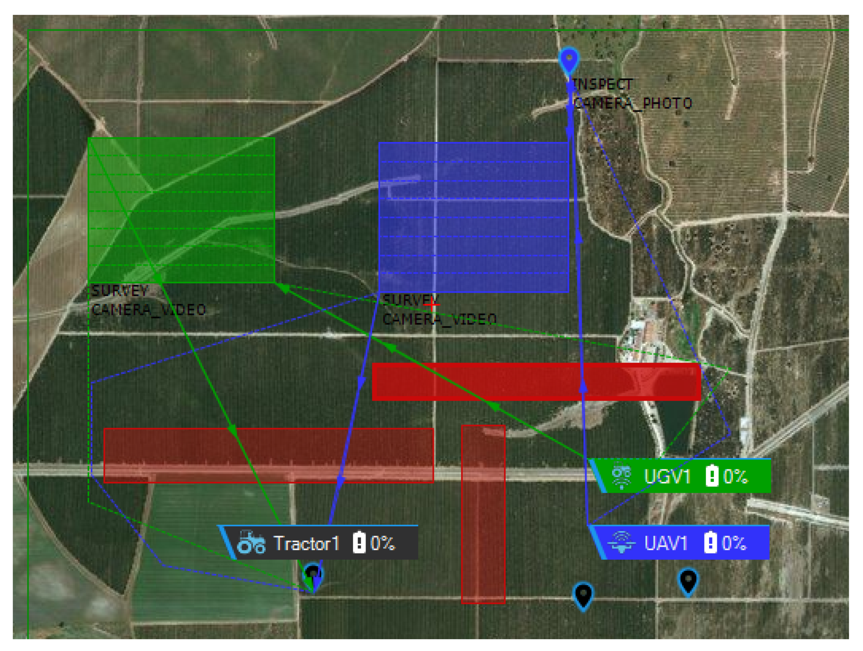
We conducted practical testing of the proposed algorithm in an actual agricultural context to assess its effectiveness, and the findings are quite promising. The algorithm successfully computes dashed-line paths that adeptly navigate around red square obstacles, showcasing its ability to avoid obstacles effectively, as shown in Figure 6. While our adaptive cellular decomposition method is capable of handling non-convex obstacles, as shown in our tests, future work will involve more rigorous testing on a wider variety of complex maps with highly irregular and non-orthogonal obstacle shapes to further validate its robustness and efficiency.

Future work will focus on extending and enhancing the proposed framework in several critical dimensions to improve its practicality, adaptability, and performance. First, we aim to conduct comprehensive and rigorous evaluations of the system across a broader range of complex and realistic environments. These environments will include maps with intricate layouts and highly irregular, non-orthogonal obstacle geometries to assess the robustness and generalization capabilities of the cellular decomposition method under diverse spatial constraints. Special attention will be given to testing in environments where traditional grid-based decomposition techniques tend to fail or become computationally expensive.

Second, a key direction involves adapting the algorithm for operation in dynamic and partially known environments. This includes integrating real-time sensory inputs, such as LiDAR or camera-based SLAM, to detect and classify previously unknown or moving obstacles. To maintain efficient path planning under such conditions, we will develop strategies for incremental map updates and localized path replanning, minimizing the need to recompute the full path from the start. This will enhance the system’s responsiveness and enable real-time autonomy in cluttered, unpredictable domains.

Furthermore, we plan to explore the scalability and extension of the framework to 3D environments, which are vital for aerial drones, underwater vehicles, and mobile manipulators. This transition from 2D to 3D introduces challenges in decomposition, memory storage, and path planning due to increased computational complexity and the need for three-dimensional obstacle avoidance. We will investigate how the adaptive decomposition method can be reformulated in 3D space while preserving its efficiency and modularity.

Lastly, another promising research direction is the deployment of this framework in multi-robot systems, where collaboration and conflict resolution are essential. In such systems, we will focus on decentralized planning architectures, enabling each agent to independently access and utilize precomputed inter-cell paths for coordination. We aim to design efficient mechanisms for communication, shared memory access, and dynamic task allocation, ensuring robust operation even in partially connected networks. This would enable robots to collaboratively explore, map, and act within complex environments while avoiding collisions and maximizing overall mission efficiency.

References

1. Mehmet, G. Dynamic Path Planning via Dueling Double Deep Q-Network (D3QN) with Prioritized Experience Replay. Appl. Soft Comput. 2024, 158, 111503. [Google Scholar]
2. Aatif, M.; Adeel, U.; Basiri, A.; Mariani, V.; Iannelli, L.; Glielmo, L. Deep Learning Based Path-Planning Using CRNN and A* for Mobile Robots. In Proceedings of the International Conference on Interactive Collaborative Robotics, Baku, Azerbaijan, 25–29 October 2023; Springer: Cham, Switzerland, 2023; pp. 118–128. [Google Scholar]
3. LaValle, S.M. Planning Algorithms; Cambridge University Press: Cambridge, UK, 2006. [Google Scholar]
4. Yao, M.; Zhao, M. Unmanned aerial vehicle dynamic path planning in an uncertain environment. Robotica 2015, 33, 611–621. [Google Scholar] [CrossRef]
5. Pretto, A.; Aravecchia, S.; Burgard, W.; Chebrolu, N.; Dornhege, C.; Falck, T.; Fleckenstein, F.; Fontenla, A.; Imperoli, M.; Khanna, R.; et al. Building an Aerial-Ground Robotics System for Precision Farming. arXiv 2019, arXiv:1911.03098. [Google Scholar]
6. Tamar, A.; Wu, Y.; Thomas, G.; Levine, S.; Abbeel, P. Value iteration networks. arXiv 2016, arXiv:1602.02867. [Google Scholar]
7. Xiao, Z.; Wan, H.; Zhuo, H.H.; Lin, J.; Liu, Y. Representation learning for classical planning from partially observed traces. arXiv 2019, arXiv:1907.08352. [Google Scholar]
8. Mourikis, A.I.; Roumeliotis, S.I. A multi-state constraint Kalman filter for vision-aided inertial navigation. In Proceedings of the 2007 IEEE International Conference on Robotics and Automation, Rome, Italy, 10–14 April 2007; pp. 3565–3572. [Google Scholar]
9. Borenstein, J.; Koren, Y. The vector field histogram-fast obstacle avoidance for mobile robots. IEEE Trans. Robot. Autom. 1991, 7, 278–288. [Google Scholar] [CrossRef]
10. Noreen, I.; Khan, A.; Habib, Z. Optimal path planning using RRT* based approaches: A survey and future directions. Int. J. Adv. Comput. Sci. Appl 2016, 7, 97–107. [Google Scholar] [CrossRef]
11. Stachniss, C.; Grisetti, G.; Burgard, W. Information gain-based exploration using rao-blackwellized particle filters. In Proceedings of the Robotics: Science and Systems, Cambridge, MA, USA, 8–11 June 2005; Volume 2, pp. 65–72. [Google Scholar]
12. Pathak, D.; Agrawal, P.; Efros, A.A.; Darrell, T. Curiosity-driven exploration by self-supervised prediction. In Proceedings of the International Conference on Machine Learning, PMLR, Sydney, Australia, 6–11 August 2017; pp. 2778–2787. [Google Scholar]
13. Richter, S.R.; Vineet, V.; Roth, S.; Koltun, V. Playing for data: Ground truth from computer games. In Computer Vision–ECCV 2016, Proceedings of the 14th European Conference, Amsterdam, The Netherlands, 11–14 October 2016; Proceedings, Part II; Springer: Cham, Switzerland, 2016; pp. 102–118. [Google Scholar]
14. Mellinger, D.; Kumar, V. Minimum snap trajectory generation and control for quadrotors. In Proceedings of the 2011 IEEE International Conference on Robotics and Automation, Shanghai, China, 9–13 May 2011; IEEE: Piscataway, NJ, USA, 2011; pp. 2520–2525. [Google Scholar]
15. Thrun, S.; Hahnel, D.; Ferguson, D.; Montemerlo, M.; Triebel, R.; Burgard, W.; Baker, C.; Omohundro, Z.; Thayer, S.; Whittaker, W. A system for volumetric robotic mapping of abandoned mines. In Proceedings of the 2003 IEEE International Conference on Robotics and Automation (Cat. No.03CH37422), Taipei, Taiwan, 14–19 September 2003; Volume 3, pp. 4270–4275. [Google Scholar] [CrossRef]
16. Hsu, D.; Kindel, R.; Latombe, J.C.; Rock, S. Randomized kinodynamic motion planning with moving obstacles. Int. J. Robot. Res. 2002, 21, 233–255. [Google Scholar] [CrossRef]
17. Melchior, N.A.; Simmons, R. Particle RRT for path planning with uncertainty. In Proceedings of the 2007 IEEE International Conference on Robotics and Automation, Rome, Italy, 10–14 April 2007; IEEE: Piscataway, NJ, USA, 2007; pp. 1617–1624. [Google Scholar]
18. Hart, P.E.; Nilsson, N.J.; Raphael, B. A formal basis for the heuristic determination of minimum cost paths. IEEE Trans. Syst. Sci. Cybern. 1968, 4, 100–107. [Google Scholar] [CrossRef]
19. Lerner, J.; Wagner, D.; Zweig, K. Algorithmics of Large and Complex Networks: Design, Analysis, and Simulation; Springer: Berlin/Heidelberg, Germany, 2009; Volume 5515. [Google Scholar]
20. Scerri, P.; Reed, N. Designing Agents for Systems with Adjustable Autonomy; Citeseer: University Park, PA, USA, 2001. [Google Scholar]
21. Zieba, S.; Polet, P.; Vanderhaegen, F.; Debernard, S. Principles of adjustable autonomy: A framework for resilient human–machine cooperation. Cogn. Technol. Work 2010, 12, 193–203. [Google Scholar] [CrossRef]
22. Schroeder de Witt, C.A.; Foerster, J.N.; Farquhar, G.; Torr, P.H.; Boehmer, W.; Whiteson, S. Multi-agent common knowledge reinforcement learning. arXiv 2018, arXiv:1810.11702. [Google Scholar]
23. Peysakhovich, A.; Kroer, C.; Lerer, A. Robust multi-agent counterfactual prediction. In Proceedings of the Advances in Neural Information Processing Systems, Vancouver, BC, Canada, 8–14 December 2019; pp. 3077–3087. [Google Scholar]
24. Kim, C.; Kim, C. Development of autonomous driving and motion control system for a patient transfer robot. Actuators 2023, 12, 106. [Google Scholar] [CrossRef]
25. Wang, T.; Li, A.; Guo, D.; Du, G.; He, W. Global dynamic path planning of agv based on fusion of improved a* algorithm and dynamic window method. Sensors 2024, 24, 2011. [Google Scholar] [CrossRef]
26. Zhang, S.; Zhao, T. Mobile robot path planning in 2d space: A survey. Highlights Sci. Eng. Technol. 2022, 16, 279–289. [Google Scholar] [CrossRef]
27. Zhang, H.; Tao, Y.; Zhu, W. Global path planning of unmanned surface vehicle based on improved a-star algorithm. Sensors 2023, 23, 6647. [Google Scholar] [CrossRef] [PubMed]
28. Zheng, C.; Kuang, M. Scouting robot with search-space reducing hybrid networks for unknown environment path planning. J. Stud. Res. 2023, 12, 1–12. [Google Scholar] [CrossRef]
29. Li, Y.; Li, J.; Zhou, W.; Yao, Q.; Nie, J.; Qi, X. Robot path planning navigation for dense planting red jujube orchards based on the joint improved a* and dwa algorithms under laser slam. Agriculture 2022, 12, 1445. [Google Scholar] [CrossRef]
30. Wesson, J.A. Sawtooth oscillations. Plasma Phys. Control. Fusion 1986, 28, 243. [Google Scholar] [CrossRef]
31. Yang, K. Anytime synchronized-biased-greedy rapidly-exploring random tree path planning in two dimensional complex environments. Int. J. Control Autom. Syst. 2011, 9, 750–758. [Google Scholar] [CrossRef]
32. Tang, S.H.; Yeong, C.F.; Su, E.L.M. Comparison between Normal Waveform and Modified Wavefront Path Planning Algorithm for Mobile Robot. Appl. Mech. Mater. 2014, 607, 778–781. [Google Scholar] [CrossRef]
33. Botea, A.; Müller, M.; Schaeffer, J. Near optimal hierarchical path-finding. J. Game Dev. 2004, 1, 1–30. [Google Scholar]
Figure 1. Proposed AA framework and output for path planning using dynamic programming.
Information 16 00700 g001
Figure 2. Output of path planning using AA for M1.
Information 16 00700 g002
Figure 3. Maps used for the simulations.
Information 16 00700 g003
Figure 4. Execution time comparison of path-planning strategies for Map 1 (logarithmic scale).
Information 16 00700 g004
Figure 5. Bar charts comparing the performance of A*, Improved A*, and RRT algorithms across 9 maps.
Information 16 00700 g005
Figure 6. Real agricultural scenario.
Information 16 00700 g006