Article

Machine Learning for Breast Cancer Detection with Dual-Port Textile UWB MIMO Bra-Tenna System

by
Azza H. Elnaggar
1,
Anwer S. Abd El-Hameed
2,*,
Mohamed A. Yakout
3 and
Nihal F. F. Areed
3
1
Communication and Electronics Engineering Department, Higher Institute of Engineering and Technology Kafer Elshiekh, Kafer Elshiekh 6862030, Egypt
2
Electronics Research Institute, Cairo 12622, Egypt
3
Faculty of Engineering, Mansura University, Mansura 35516, Egypt
*
Author to whom correspondence should be addressed.
Information 2024, 15(8), 467; https://doi.org/10.3390/info15080467
Submission received: 10 June 2024 / Revised: 2 August 2024 / Accepted: 2 August 2024 / Published: 6 August 2024

Abstract

:
A wearable textile bra-tenna system based on dual-polarization sensors for breast cancer (BC) detection is presented in this paper. The core concept behind our work is to investigate which type of polarization is most effective for BC detection, using the combination of orthogonal polarization signals with machine learning (ML) techniques to enhance detection accuracy. The bra-tenna sensors have a bandwidth ranging from 2–12 GHz. To complement the proposed system, detection based on machine learning algorithms (MLAs) is developed and tested to enhance its functionality. Using scattered signals at different polarizations, the bra-tenna system uses MLAs to predict BC in its early stages. Classification techniques are highly effective for data classification, especially in the biomedical field. Two scenarios are considered: Scenario 1, where the system detects a tumor or non-tumor, and Scenario 2, where the system detects three classes of one, two, and non-tumors. This confirms that MLAs can detect tumors as small as 10 mm. ML techniques, including eight algorithms such as the Support Vector Machine (SVM), Random Forest (RF), Gradient Boosting Methods (GBMs), Decision Tree (DT) classifier, Ada Boost (AD), CatBoost, Extreme Gradient Boosting (XG Boost), and Logistic Regression (LR), are applied to this balanced dataset. For optimal analysis of the BC, a performance evaluation is performed. Notably, SVM achieves outstanding performance in both scenarios, with metrics such as its F1 score, recall, accuracy, receiver operating characteristic (ROC) curve, area under the ROC curve (AUC), and precision all exceeding 90%, helping doctors to effectively investigate BC. Furthermore, the Horizontal-Horizontal (HH) sensor configuration achieved the highest accuracy of 98% and 99% for SVMs in the two scenarios, respectively.

1. Introduction

Breast cancer is a significant global concern, often described as the leading cause of death among women in urban areas [1]. The Centers for Disease Control and Prevention (CDC), a reliable source, states that BC is most likely the sickness that kills women worldwide. Early detection is the best way to increase the chance of treatment and survivability. The abnormal growth of the breast cells can lead to cancers in women. Depending on the region, size and position, these enormous tumor cells split into cancerous and normal cells [2]. The initial tumor region of the noncancerous tumor is referred to as benign, whereas the secondary tumor area of the cancerous tumor is referred to as malignant. Benign tumors do not pose a threat to women’s lives because they are treatable and can be made to grow more slowly with the appropriate care. The patient must obtain the required medical attention, such as radiation therapy or surgery, to treat a malignant tumor. A computerized diagnostic system using an ML approach was required because the current tests for detecting BC, such as mammography, ultrasound, and biopsy, were time-consuming. Among the algorithms used in this technique are those that aid in tumor categorization, improve cell detection accuracy, and reduce processing time.
In recent years, tremendous growth in artificial intelligence (AI) has been seen, particularly ML, in the context of data analysis and computing, which often enables programs to operate intelligently [3]. Classification is a crucial and fundamental task in ML and data mining. Significant research efforts have been dedicated to applying these techniques to a variety of medical datasets for BC classification.
ML is a common term for the newest technologies in the fourth industrial revolution (also known as Industry 4.0), which generally gives systems the capacity to learn and improve from experience automatically without having to be expressly programmed [4,5]. Therefore, MLA is essential for both the intelligent analysis of these data and the creation of the associated real-world applications. Four main types of learning algorithms may be distinguished in this domain: supervised, unsupervised, semi-supervised, and reinforcement learning [6]. The success and efficiency of ML solutions depend significantly on both the nature and quality of the data, as well as the capabilities of the learning algorithms used. To successfully create data-driven systems, ML algorithms can be used in the areas of classification analysis, regression, data clustering, feature engineering, dimensionality reduction, association rule learning, or reinforcement learning [7,8]. It is, therefore, difficult to choose an appropriate learning algorithm that fits the intended application in a given area. The explanation for this is that various learning algorithms have distinct goals, and even within the same category, the results of various ML algorithms might differ based on the properties of the data [9,10,11,12,13,14]. Therefore, it is critical to comprehend the tenets of various MLAs and how they apply to a range of real-world application domains, including sustainable agriculture, internet of things (IOT) systems, cyber security services, business and recommendation systems, smart cities, healthcare, COVID-19, and BC [15,16,17,18,19,20,21]. Many prior studies have employed ML techniques, such as LR, DT, SVM, etc., which offer a more convincing representation [22,23,24,25,26,27,28].
Some of the related earlier research on BC diagnosis that was conducted by scientists employing various ML techniques have been discussed. Researchers employed ML approaches for data categorization and interpretation to enhance the functionality of microwave detection systems [29,30,31,32,33,34,35,36,37,38,39]. There are methodological flaws in the study [40], including the algebraic combining of microwave signals’ phase and magnitude, potentially resulting in poorer tumor identification. The authors’ decision to apply standardization without clear justification is questionable. The limited sample size of 366 samples may not be representative of the population, impacting the generalizability of the results. The method also shows poor accuracy, highlighting the need for a more sophisticated approach. In [41], the study presents a promising method for detecting BC using XG Boost but faces methodological issues. The unbalanced dataset may lead to biased results, and the author’s use of the synthetic minority over-sampling technique (SMOTE) has drawbacks, including amplification of biases and noise. The study also lacks evidence supporting SMOTE as the best approach to resolving class imbalance, suggesting a more comprehensive strategy should compare outcomes of other techniques and assess their effectiveness. The outcome classifications, including KNN, SVM, RF, and DT, were reported [42]. The Wisconsin Breast Cancer (WBC) dataset was utilized, and it was sourced from the UCI repository. According to the simulation findings, SVM, RF, DT, and KNN were the best classifiers.
The University of Wisconsin Hospital’s Dr. William H. Walberg’s dataset was utilized in [43,44]. This imbalanced WBC dataset was subjected to several data visualization and ML approaches, such as LR, KNN, SVM, naïve Bayes (NB), DT, RF, and rotation forest. These ML methods and their visualizations were to be implemented using R, Minitab, and Python. However, it is critical to pre-process the dataset before running the algorithm. Three ML approaches—SVM, RF, and Bayesian networks (BNs), were the subjects of a comparative study in [45]. The training set was the original WBC data collection. The results of the simulation demonstrate that the chosen approach affects the classification performance. SVMs perform best in terms of accuracy, specificity, and precision, according to the results. On the other hand, RFs have the best chance of accurately diagnosing tumors despite the analysis and evaluation of numerous predictors of BC recurrence risk and various types of ML algorithms.
In this paper, the central focus of our research is to explore the most effective type of polarization for BC detection. We achieve this by combining orthogonal polarization signals with ML techniques to improve detection accuracy. We provide a thorough understanding of the ML algorithm for the dataset acquired by the innovative bra-tenna system, which is used to improve the intelligence and functionality of BC detection. This system comprises four dual-polarized sensors in which each sensor has the ability to transmit/receive a microwave signal in both horizontal and vertical polarizations ranging from 2–12 GHz. Eight distinct ML techniques are investigated for BC diagnosis. The first step is to collect the dataset from a vector network analyzer (VNA). The next step involves data pre-processing, which is performed to improve the quality of a dataset to obtain clean data that can be useful for modeling. During the data pre-processing stage, the data are divided into the training and the test datasets. Furthermore, two scenarios are analyzed: the first one is the differentiation between one tumor and no tumor, and the second one is the distinguishing between one, two, and no tumors. Our approach performs better than existing methods, demonstrating microwave detection potential as a useful tool for the diagnosis of BC. A competitive performance was demonstrated when dealing with a balanced dataset above (90% accuracy).

2. Wearable Orthogonal-Polarized MIMO Bra-Tenna System

The sensor design significantly influences the overall performance of the microwave BC detection system. It is crucial for the sensor element to demonstrate broadband behavior, enabling the radiation of pulses across a wide frequency range with high fidelity and a reasonable level of gain. By optimizing the size of the individual sensor element, larger arrays can be constructed, thereby capturing more information from the scattered signals for effective detection. Implementing ultra-wide band (UWB) technology aids in creating a high-resolution system and minimizing distortion in the transmission of short-duration pulses.

2.1. Sensor Design

Figure 1 shows the proposed UWB textile multi-input multi-output (MIMO) sensor’s geometrical structure with orthogonal polarization [46]. It is recommended that the feeding structure be CPW-fed for ease of manufacture and integration. The proposed design primarily consists of a partial ground plane, a feeding network, and a radiating corrugated half-circle. Impedance matching is improved by using the partially grounded plane. To further enhance the impedance matching over the whole band, the CPW feeding structure’s signal line is tapered with W t = 2.5 mm. An extensive out-of-band rejection is achieved by using a strip line that functions as a low-pass filter (LPF) to reduce the reciprocal coupling between the sensor’s radiating elements [47]. Located in between the two monopole sensors, this LPF is made of conducting fabric. Mutual coupling is successfully reduced when the stop band characteristics of the LPF match with the sensor’s operating frequency, therefore almost completely blocking the passage of the generated signal between the two parts. The potential sensor is designed and constructed with dimensions of L = 60 mm and W = 70 mm. It is based on a flexible textile substrate with dielectric permittivity of ε r = 1.8, a loss tangent of 0.025, and a thickness of h = 0.3 mm.

2.2. Sensor Fabrication and Results

A laser cutting machine is used to produce the suggested pattern utilizing conductive copper nanoparticles on a textile substrate. Figure 2a shows the wearable sensor prototype. The adhesive-coated conductive fabric may be pressed straight onto the dielectric fabric that will be included. When the SMA connection is connected, the textile-based MIMO wearable sensor also entirely avoids heat. Rather than using epoxy glue, conductive adhesive is utilized to connect the recommended sensor for measurement. The reflection coefficient data from the experiment and simulation are compared in Figure 2b,c. The simulated and fabric textile sensors produced good impedance matching. The proposed textile antenna has a stated −10 dB impedance bandwidth from 2.5 to 12 GHz, covering the whole simulated 3.5–11.65 GHz UWB spectrum. However, there are some slight discrepancies because of things like SMA connections, manufacturing tolerances, and soldering errors that were not considered in the simulations.

2.3. Wearable BC Monitoring System

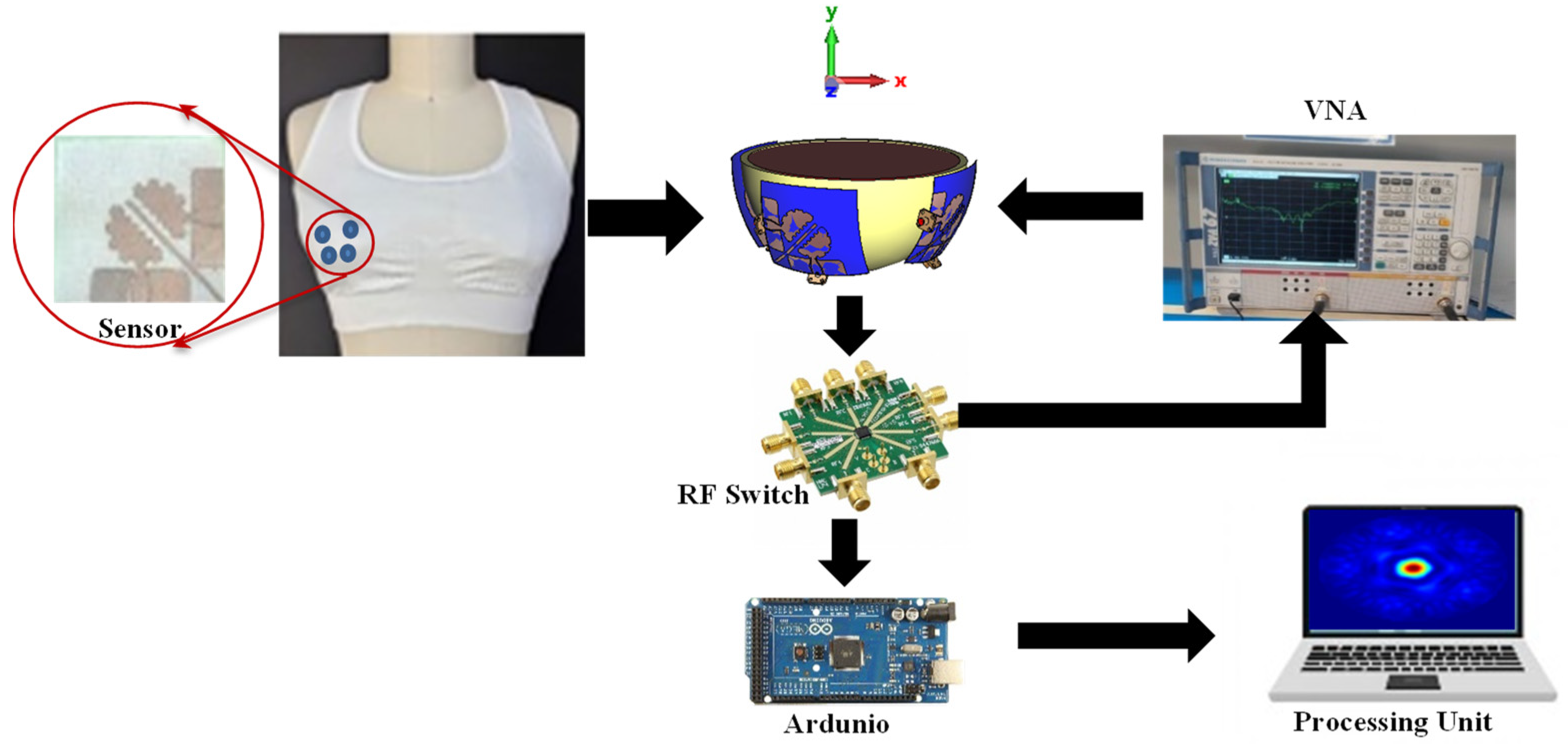
Figure 3 presents the schematic diagram of the proposed BC detection system, showcasing a novel, comfortable, wearable solution tailored for regular and safe BC screening in women. The system utilizes textile-based sensors seamlessly integrated into a woman’s bra for easy attachment. The schematic highlights the compact design of the wearable orthogonal-polarized bra-tenna MIMO sensor, responsible for transmitting and receiving UWB signals, along with an electrical 9-port RF switch and data acquisition facilitated through a VNA. Control and coordination of the entire system are facilitated by a personal computer (PC) and an Arduino kit, responsible for signal processing and executing reconstruction algorithms.
The exploited sensors were placed in pairs facing each other inside the bra system according to a predetermined calculation of the Fidelity Factor [48]. For simplicity, the breast model we utilized was built in our laboratory at the Electronics Research Institute lab (ERI) and had skin and normal cells as one layer with an average permittivity of 17. The breast model has standard dimensions with a radius of 75 mm. A spherical tumor with a 10 mm radius and permittivity of 50 is incorporated, reflecting the dimensions indicative of stage one breast cancer, which is an appropriate stage for recognition and effective therapy. In order to simulate a large number of sensors, the phantom was rotated 360° by 20° step while the sensors are kept stationary. In future work, we will consider increasing the number of antenna elements to avoid any rotation to the phantom to obtain a more reliable imaging system. Their precise locations are determined using high-precision tools, and their positioning around the breast model is critical to the design. Each antenna element is situated 6.5 cm away from the center of the phantom. Simplifying the data acquisition process, one port is directly connected to the VNA to function as a transmitter, while the other ports are linked to an RF switch, controlled by an Arduino Mega through a single PC. By altering the Tx port, the Tx position is changed, and this process is repeated for other ports using the RF switch. The backscattered signals collected fall within the frequency range of 2 to 12 GHz. We collect data for three scenarios: one tumor, two tumors, and no tumors present. Subsequently, we employ automated learning techniques to predict the presence or absence of a tumor.

3. Data Collection and Pre-Processing

The choice of which specific learning algorithm to use is a critical step. The evaluation of a classifier is most often based on prediction accuracy, which is calculated as the percentage of correct predictions divided by the total number of predictions. These techniques help us to assess the performance of a classifier and to make informed decisions about model selection.
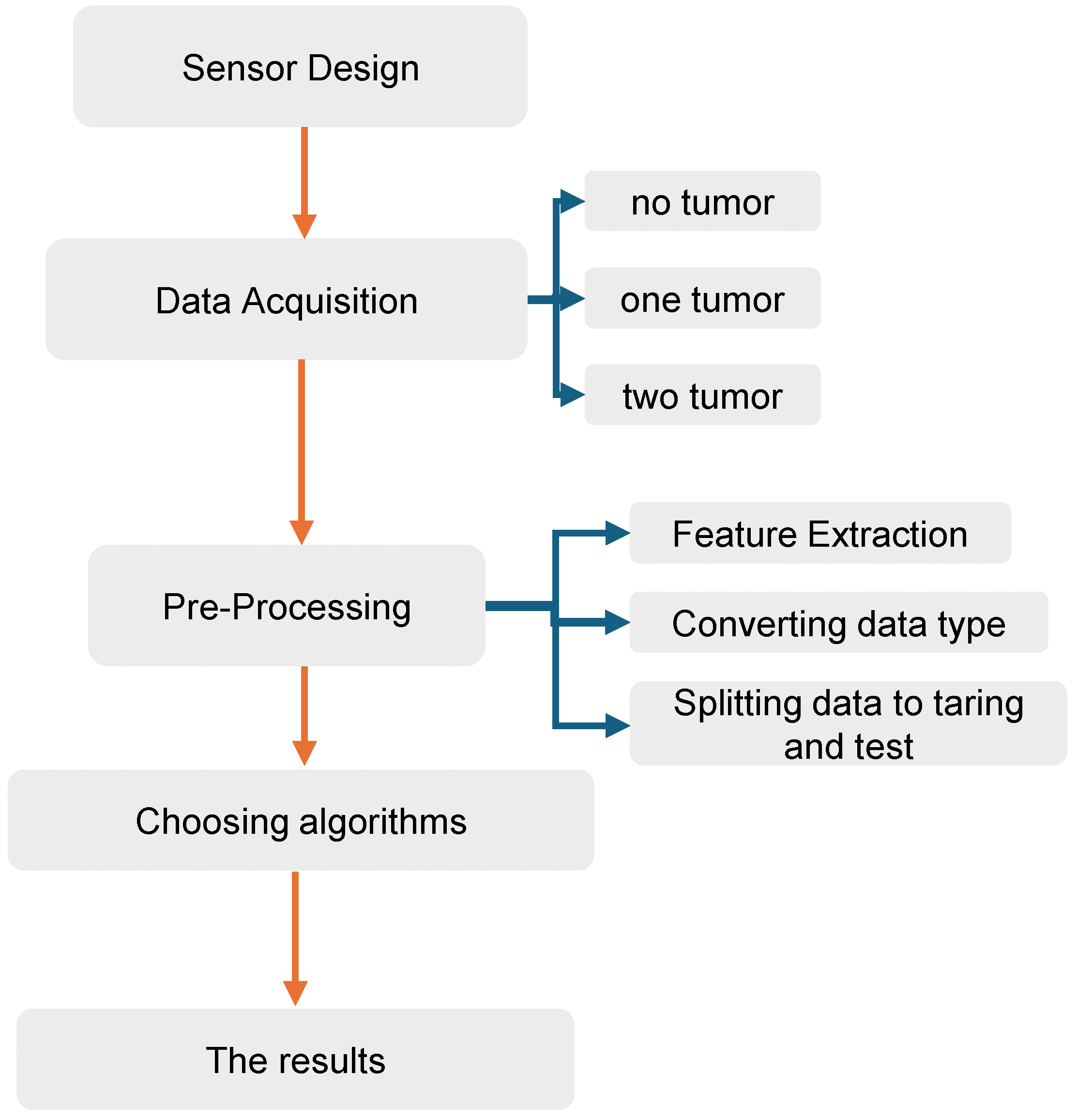
Figure 4 illustrates the proposed BC detection model and its workflow. The process begins with sensor design and data acquisition, where data are categorized into three classes: no tumor, one tumor, and two tumors. Following pre-processing, which includes feature extraction, data type conversion, and data splitting for training and testing, the model proceeds to the selection of algorithms, ultimately leading to the generation and evaluation of results.

3.1. Machine Learning Algorithms and Evaluation Metrics

The choice of which specific learning algorithm to use is a critical step in our methodology. The evaluation of the classifier is predominantly based on prediction accuracy, which is the percentage of correct predictions divided by the total number of predictions. The algorithms employed in our study, such as SVMs, RFs, GBMs, DTs, ADs, CatBoosts, XG Boosts, and LRs, will be summarized in this subsection. Their underlying principles and evaluation metrics (accuracy, precision, recall, F1 score, ROC curve, and AUC) are familiar to experts in this domain. We have indicated that the degree of rotation is the primary feature that we used in our investigation. An overview of various ML detection algorithms is given in this section with examples.
1.
Logistic Regression (LR)
The LR approach is among the most basic types of traditional ML algorithms. The fitting probability of the event on the logistic curve serves as the basis for predicting a target variable [10].
2.
Support Vector Machine (SVM)
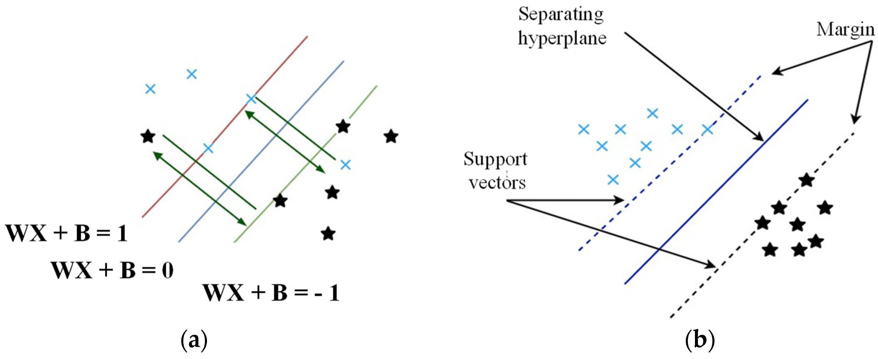
Regression and classification tasks are handled by SVMs [10,29]. It is among the most potent conventional MLAs. They work by employing a separating hyperplane to divide data into distinct classes. However, an SVM selects a plane with the largest margin—that is, the separation between data points from various classes. It can be computed as follows:
If   Y i = + 1 ; w x i + b 1 If   Y i = 1 ; w x i + b 1 For   all   i ;   y i   ( w x i + b ) 1
where, as seen in Figure 5 [15], w is a weight vector, b is a constant term that represents the distance from the origin, and x is a vector data point.
3.
Decision Trees (DTs)
DTs are extensively used in many ML applications because of their effectiveness in classification and prediction tasks [14]. A DT operates as a supervised learning algorithm that relies on a hierarchical structure to make recursive splits of nodes into finer steps. It comprises decision nodes and terminal leaves, where the decision nodes are interconnected by a predictive model, and each leaf represents a distinct class.
4.
Random Forest (RF)
A RF is a supervised learning algorithm widely used by researchers for classification tasks [16,23]. Renowned as an ensemble classification technique, it employs ensemble learning, which involves combining multiple classifiers to address complex problems.
5.
Gradient Boosting Methods (GBMs)
A GBM focuses on combining multiple decision trees, considered weak learners, to construct a strong learner for accurate predictions [17]. It utilizes gradient descent as its optimization algorithm to minimize the loss function, resulting in an improved learner. For a given loss function, φ (y, f), and a base learner, h(x, θ ). The GBM algorithm produces h(x, θ t ), which aligns with the negative gradient { g t x i } i = 1 N of the data, as described in [17]:
g t ( x ) = E y [ φ ( y , f ( x ) ) f ( x ) | x ]
f x = f t 1 ( x )
This process ultimately results in an optimized least-squares solution, which can be expressed as follows:
( ρ t , θ t ) = a r g m i n ρ , θ   Σ i = 1 N [ g t ( x i ) + ρ h ( x i , θ ) 2 ]
6.
Categorical Boost (“CatBoost”)
In this technique, both gradient boosting and categorical features are combined to create the “CatBoost” algorithm [27,28]. It employs a random permutation and one-hot-max-size encoding to emphasize categorical features, thereby enhancing the algorithm’s robustness [28]. In CatBoost, a random permutation of the dataset is performed, and an average label value is assigned to each data sample [28]. For binary classification tasks, CatBoost not only improves classification accuracy but also ensures fast training speeds.
7.
Adaptive Boosting (Ada Boost)
Ada Boost, known as an adaptive classifier, significantly enhances the efficiency of the classifier but can sometimes lead to overfitting. It is particularly effective when used to boost the performance of DTs, which serve as the base estimator [19], in binary classification problems. However, Ada Boost is sensitive to noisy data and outliers.
8.
Extreme Gradient Boosting (XG Boost)
XG Boost utilizes ensemble boosting specifically for DT algorithms [35,37]. XG Boost combines multiple weak models to produce a stronger overall model. Given different inputs and outputs, ( x 1 , y 1 ), ( x 2 , y 2 ), · · ·, ( x n , y n ), the ensemble algorithm employs (K) additive functions to predict an output, as described in [35,37]:
y i ^ = Σ k = 0 k   { f k x , f ϵ F }
where f ϵ F represents the space of classification and regression trees (CARTs). The function is approximated by minimizing a regularized objective function for a given set of parameters (q) as follows:
Obj   ( θ ) = Σ i = 0 n   l   ( y i ^ ,   y i ) + Σ k = 0 k ( f k )
Here, l( y i ^ , y i ) represents the training loss function that measures the difference between the predicted values and the actual values, while Ω ( f k ) denotes the regularization term that penalizes the complexity of the model.
In particular, accuracy measures the proportion of correctly classified instances, while recall and precision provide insight into the algorithm’s ability to detect true positives (TPs) and false positives (FPs), respectively. The F1 score, which is the harmonic mean of precision and recall, provides a balanced measure of both. The ROC curve and AUC provide a visual representation of the algorithm’s performance, with higher AUC values indicating better separation between positive and negative classes. The ROC curve provides a visual representation of the performance of each classifier, facilitating the selection of optimal models and the identification of less effective ones.
The following equations are used in performance measures of the most commonly used biological and medical accuracy, recall, precision, and F1 score.
Accuracy = T N + T P T P + T N + F P + F N   %
recall = T P ( T P + F N )   %
Precision = T P ( T P + F P )   %
F 1   score = p r e c c i s i o n × r e c a l l p r e c c i s i o n + r e c a l l × 2 %

3.2. Dataset of BC

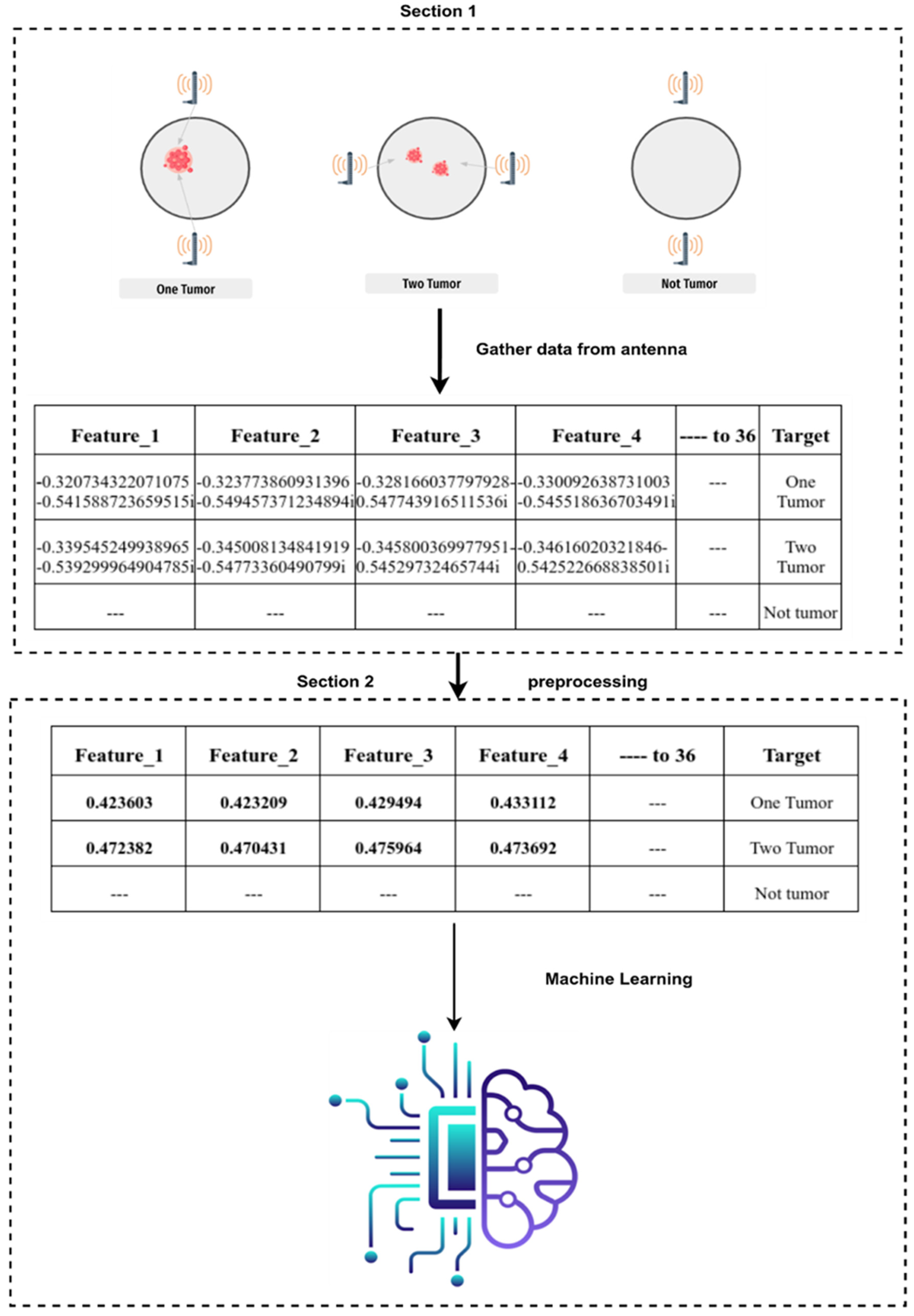
In the scenario of a balanced dataset described, four dual-polarization sensors equipped with 8 ports—comprising four horizontal and four vertical polarizations—were used to acquire HH and horizontal-vertical (HV) data for the detection of small-sized tumors. The dataset includes parameters of both s 11 and s 21 for HH and HV. The dataset of each parameter consists of 801 samples associated with their labels over frequencies from 2–12 GHz. Figure 6 outlines the methodology for gathering datasets in the BC detection. The labels are coded as 0, 1, and 2, representing none, one, and two tumors, respectively. The dataset is randomly divided into two subsets, approximately 80% for training and the remaining 20% for testing.

3.3. Pre-Processing

Pre-processing is a crucial step in preparing the data for ML model training. Upon acquiring the dataset, the next step involves pre-processing, encompassing feature extraction where relevant data attributes are identified and extracted. This is followed by converting data types for compatibility with an MLA and then splitting the data into training and test sets for model development and validation. The data tables illustrate the extracted features (Feature_1 to Feature_36) and their corresponding target labels (tumor or no tumor). In this study, we used two different pre-processing scenarios to handle the dataset.

3.3.1. Scenario 1: One Tumor or No Tumor

In the first scenario, we distinguished between breast tissue with and without tumors using two datasets: one with tumors and one without. Python was used for pre-processing. We loaded the datasets using pandas, assigning column names using the ‘names’ parameter. We then converted complex numbers to a Python-compatible format and extracted their magnitudes using numpy’s absolute function, discarding phase information. Tumor samples were labeled as 1 and non-tumor samples as 0. The datasets were concatenated and shuffled to ensure randomness. Complex data from the bra-tenna system were transformed to facilitate intuitive analysis. Complex numbers (magnitude and phase) were converted to magnitudes, capturing signal strength while ignoring phase information. The pre-processed dataset consisted of 1602 samples (tumor and non-tumor) with 36 features each. Sample datasets are shown in Table 1 and Table 2 before and after pre-processing. The pseudo-code is shown in Table 3. We developed the synthetic code to demonstrate the processing of complex-valued data in the frequency domain, a crucial aspect of our methodology. As ML algorithms typically deal with real-valued data, we devised a strategy to deal with the complex-valued measurements obtained from the bra-tenna sensor. This involved a feature extraction approach in which we computed the magnitude values of the complex measurements and combined them to form a comprehensive feature set. This process enabled us to use machine learning techniques to effectively analyze the data and detect BC.
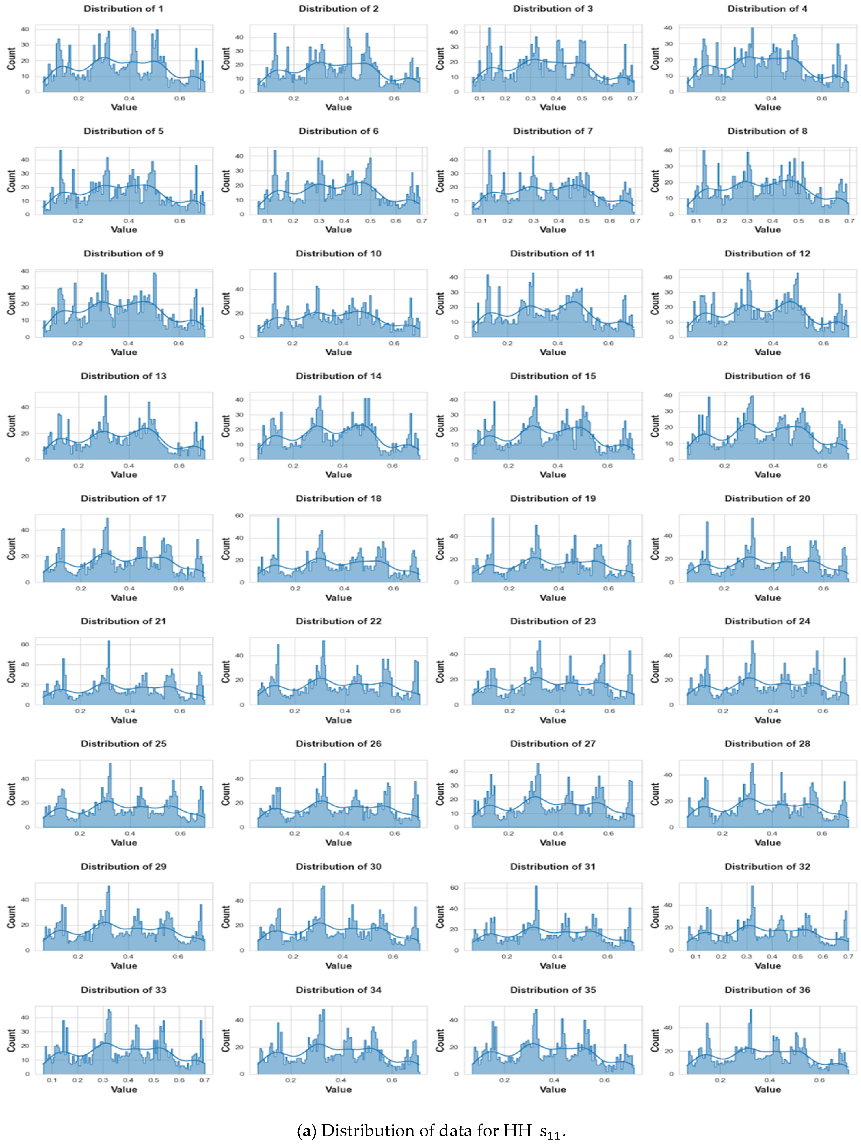
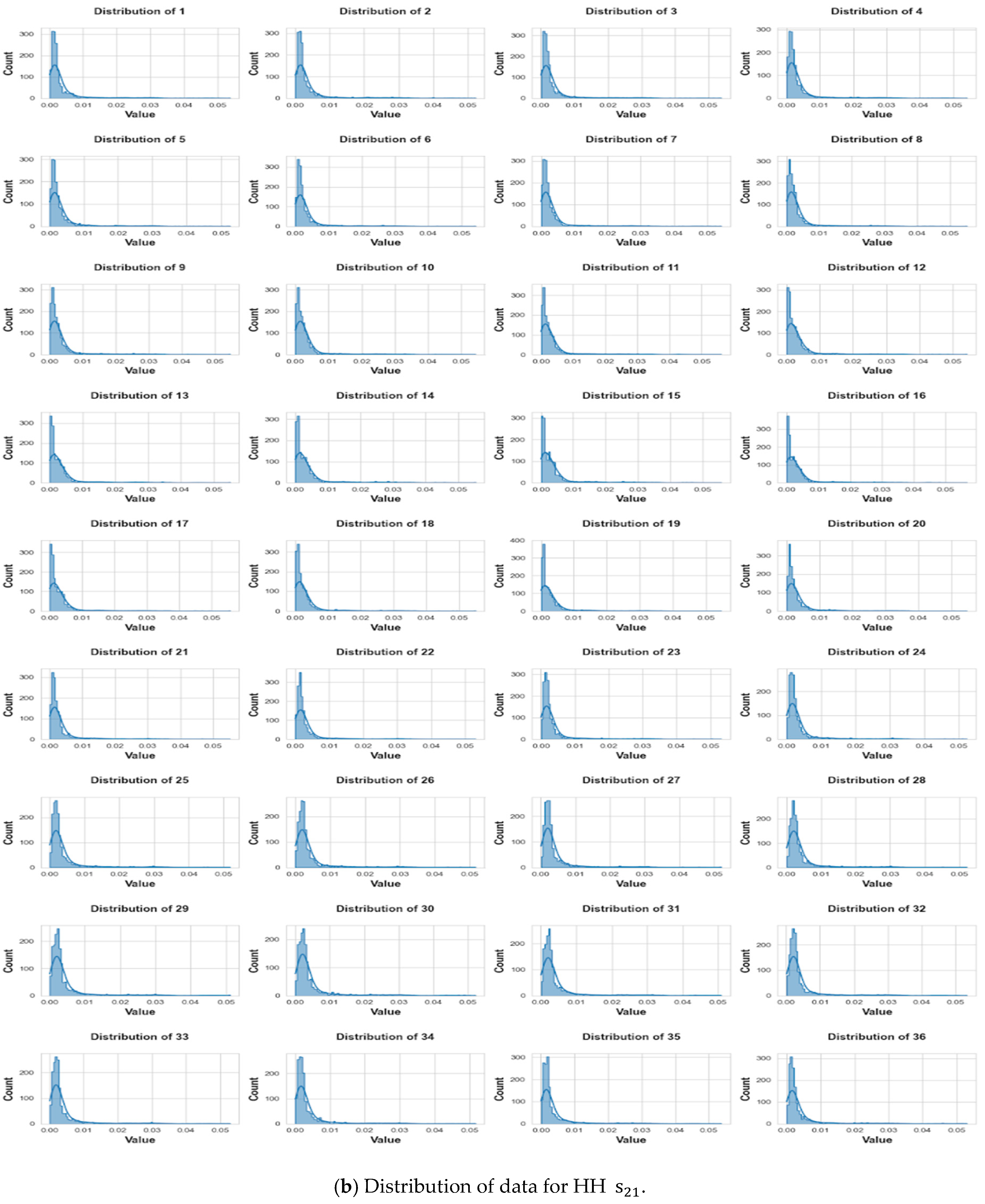
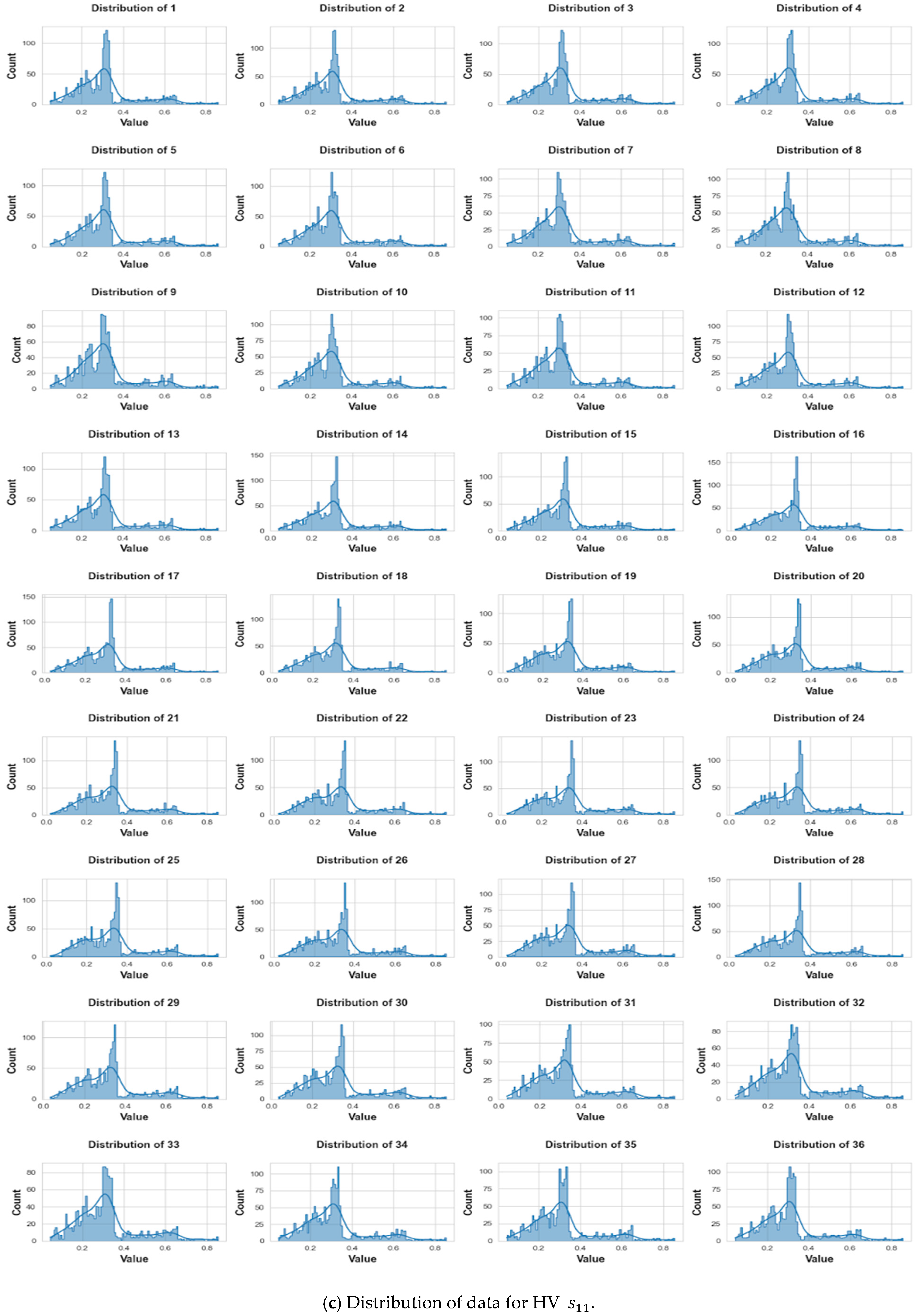
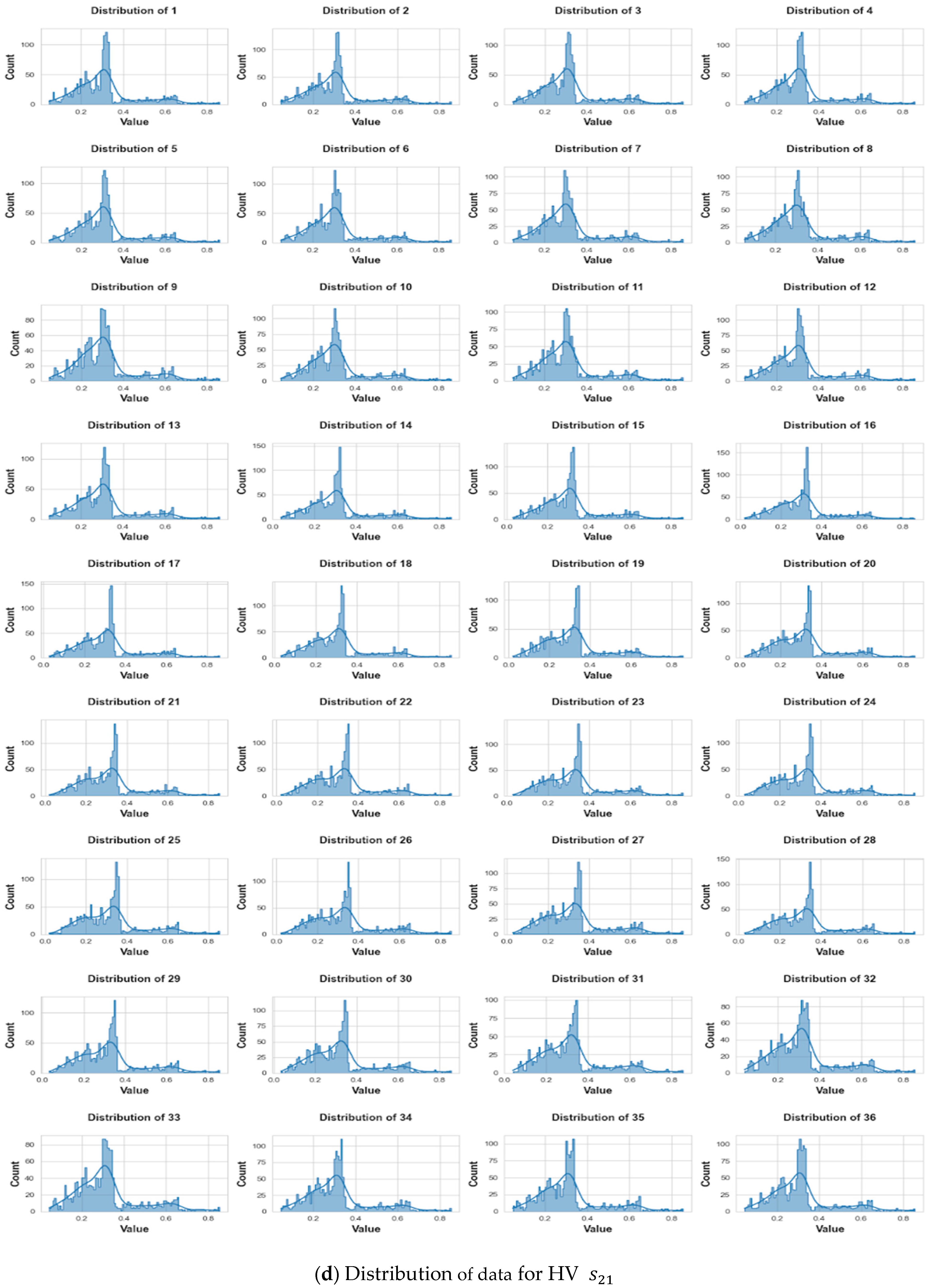
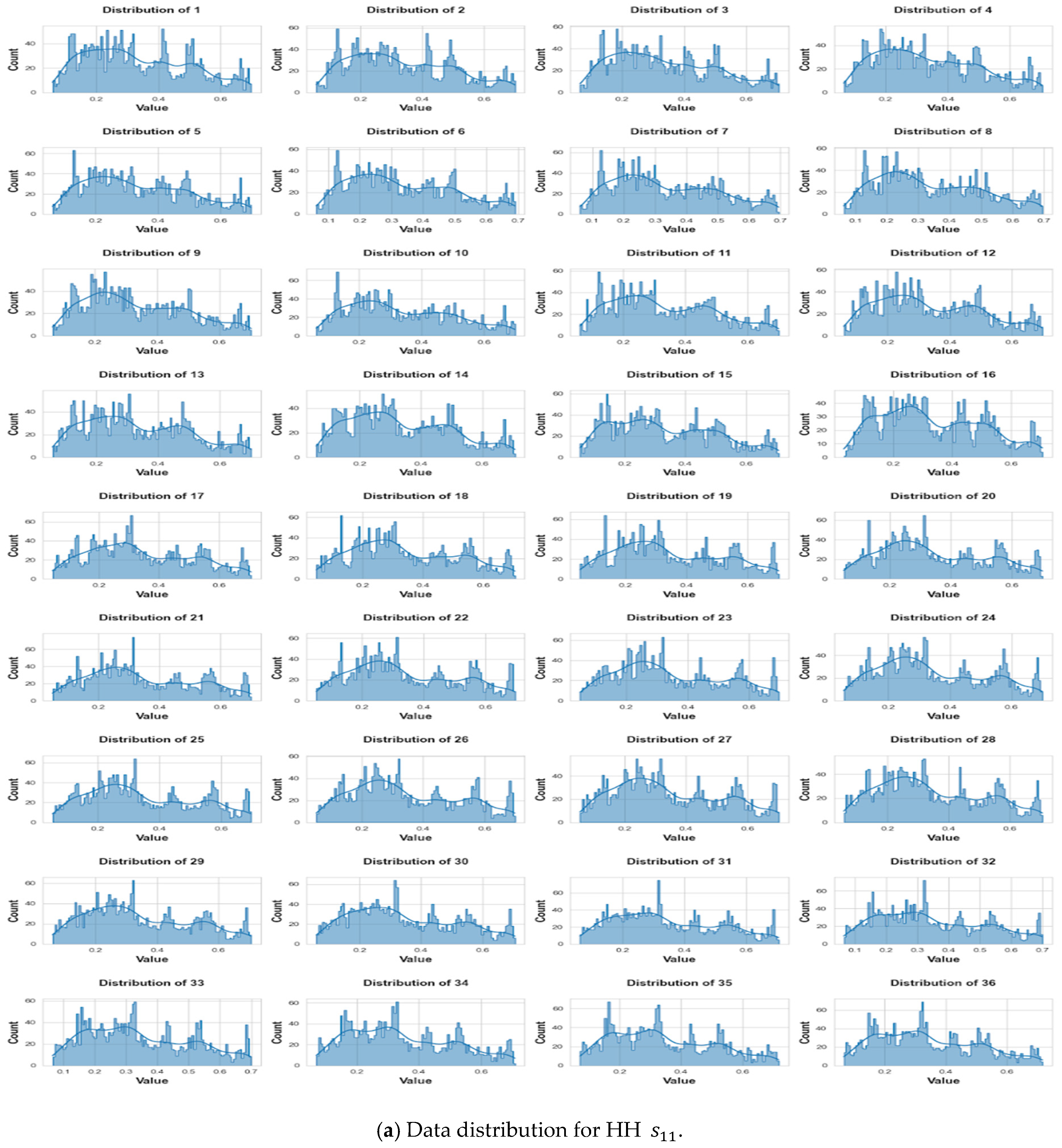
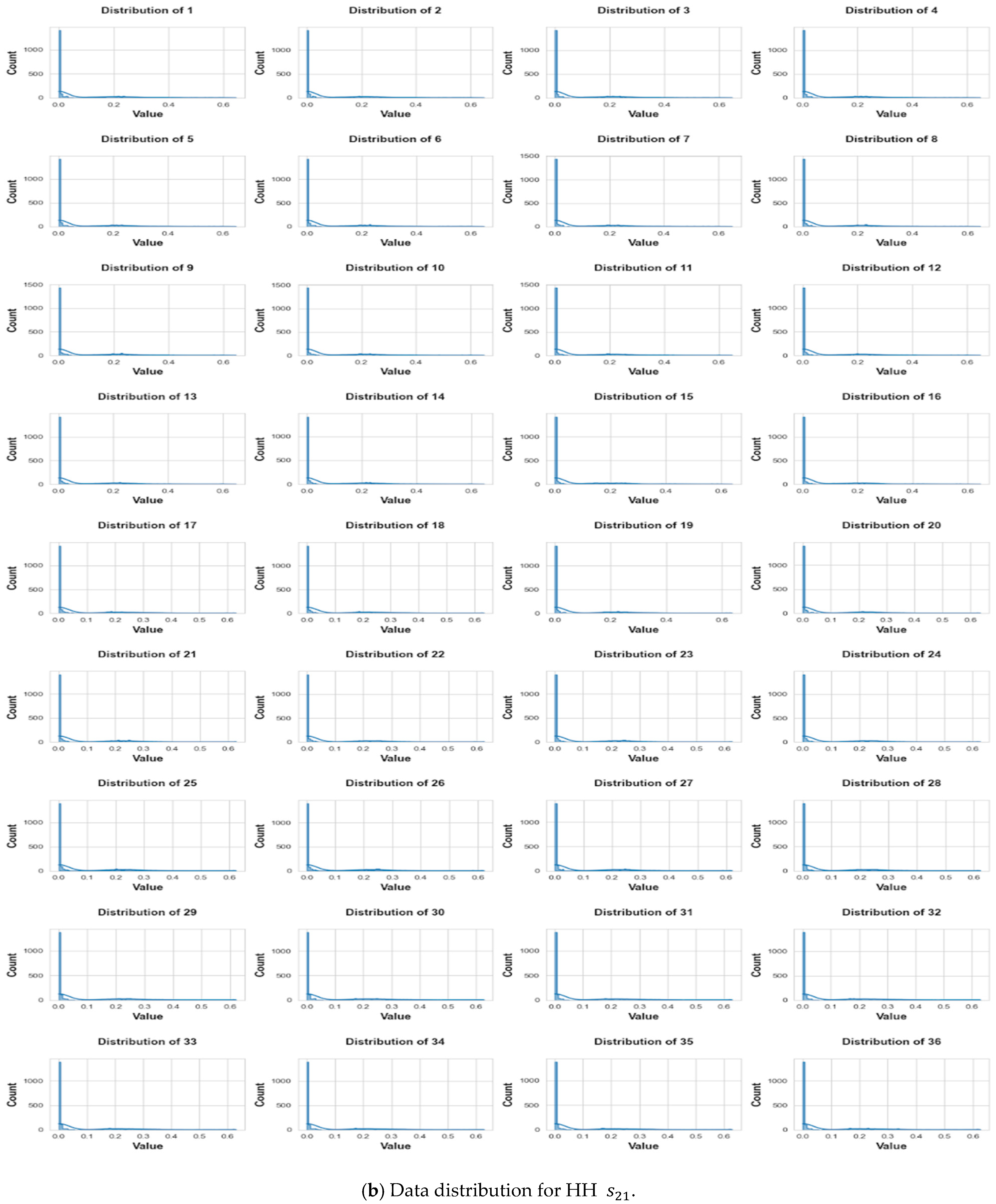
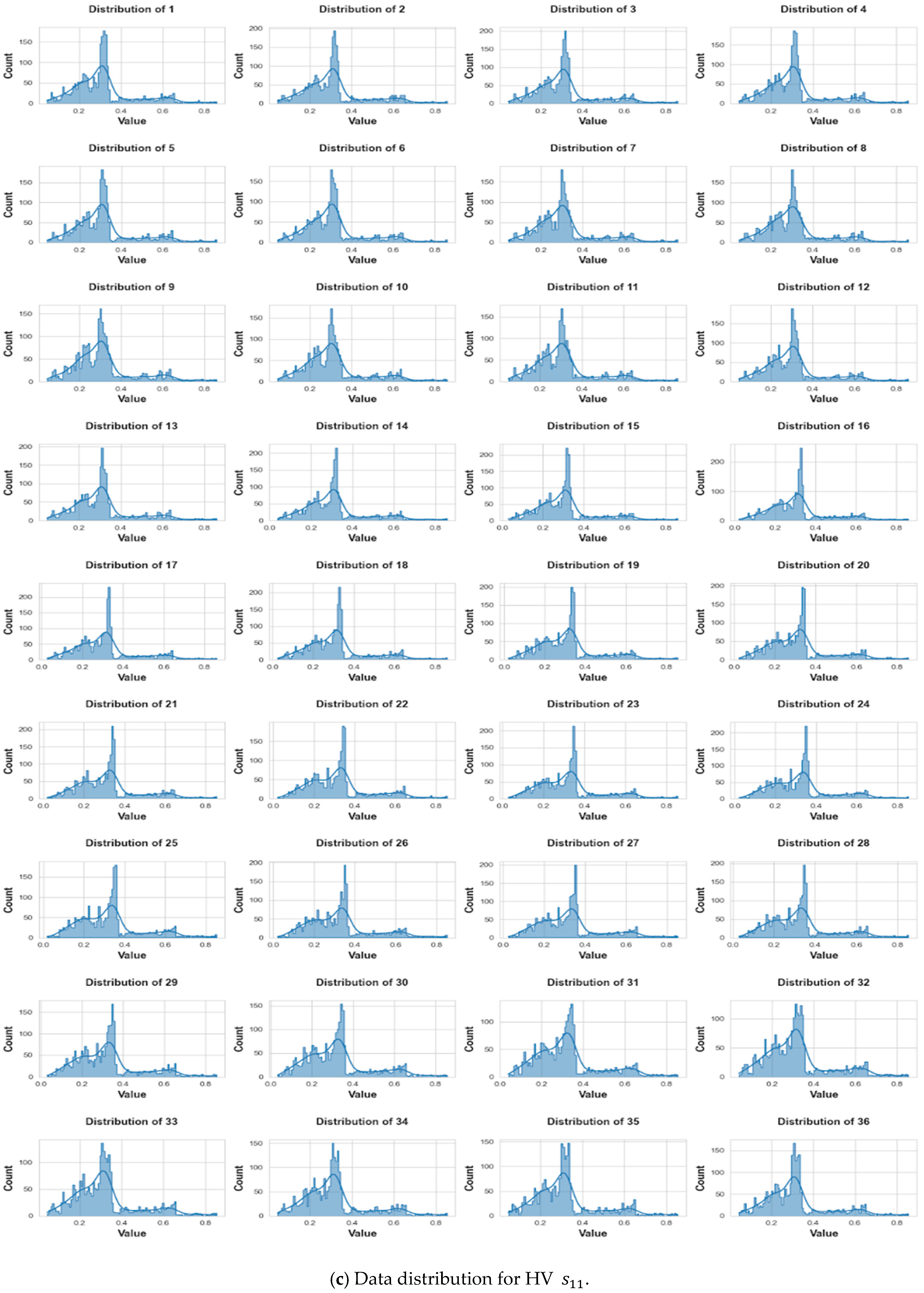
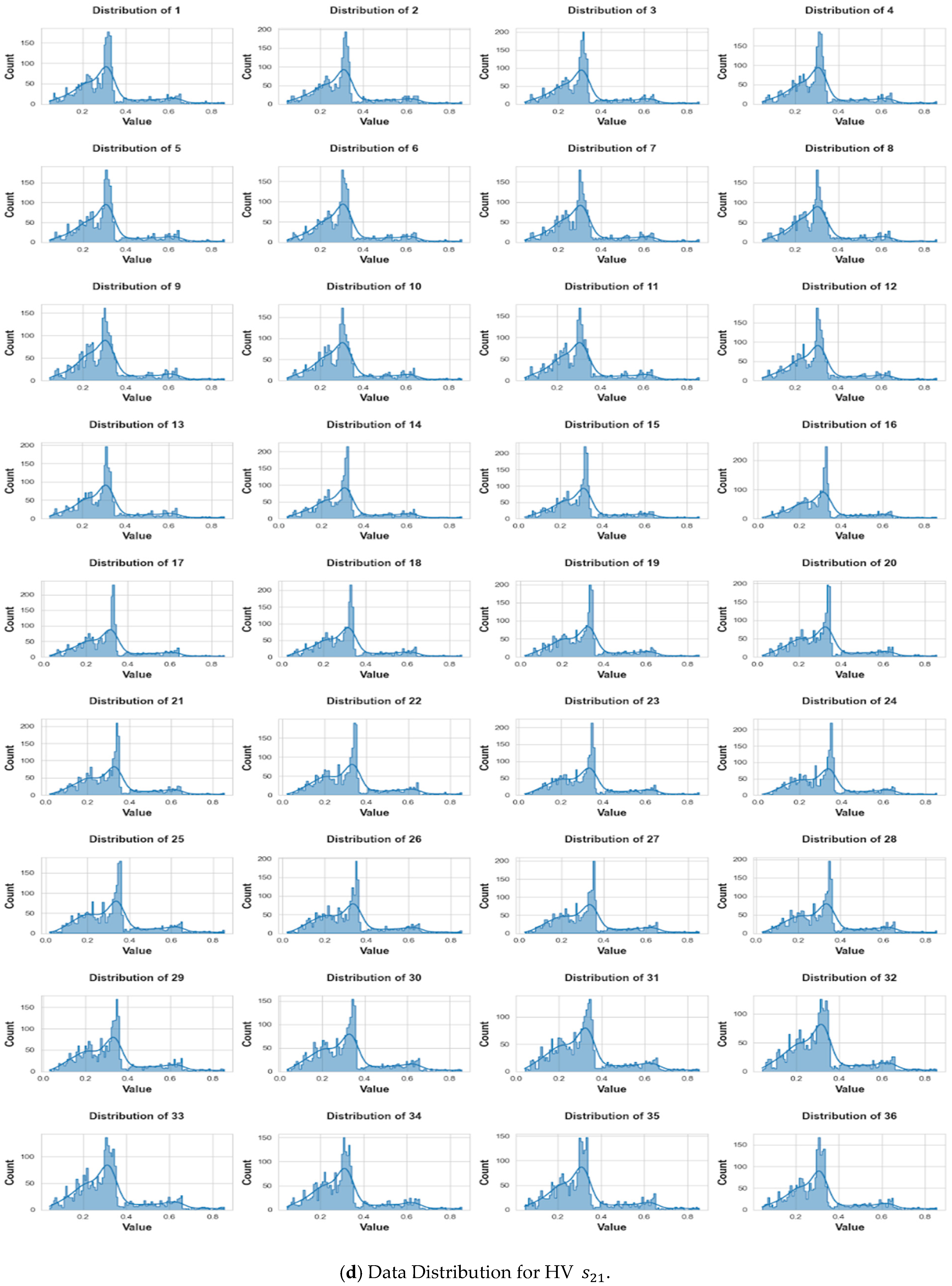
The scattering parameter distributions for the first case (one tumor, no tumor) show some interesting trends regarding polarization and signal intensity. Figure 6 shows that by visual inspection, co-polarized measurements of HH appear to have higher signal intensity than cross-polarized data HV for both s 11 and s 21 parameters. This finding is consistent with the understanding that signal cancellation is less severe in co-polarized sensor configurations than in cross-polarized ones. In addition, the HH s 21 and HV s 21 distributions shown in Figure 7b,d appear more distinct compared with the HH s 11 and HV s 11 distributions shown in Figure 7a,c. This could indicate that the application of the Horizontal-Horizontal polarization technique results in a more pronounced signal response.

3.3.2. Scenario 2: One or Two Tumors vs. No Tumor

In the second scenario, we extended our analysis to distinguish between breast tissues with one or two tumors and those without. We concatenated the datasets from Scenario 1, added an additional dataset with two tumors (2403 samples) and applied the same pre-processing steps as described in Scenario 1. The main differences in this scenario are in the label assignment and data concatenation steps. Specifically, we assigned labels as follows: 0 for no tumor, 1 for one tumor, and 2 for two tumors. We then concatenated the three datasets, resulting in a comprehensive dataset that captures the variability of breast tissue conditions. The distribution of the pre-processed data is shown in Figure 8, which highlights the different patterns and characteristics of the three classes. This visualization provides valuable insights into the underlying structure of the data and informs the development of ML models that can effectively detect the presence of small-sized tumors.
As shown in Figure 8, the results from Scenario 1 are further corroborated by examining the S-parameter distributions ( s 11 and s 21 ) in Scenario 2 (one, two, and no tumors). Co-polarized measurements (HH and HV) for s 11 , shown in Figure 8a,c, show higher signal intensities compared with s 21 , as shown in Figure 8b,d, similar to Scenario 1. In addition, the HH s 11 distributions appear more distinct than their HV counterparts.

4. Results and Discussion

This section presents a comprehensive comparative study of the performance of eight ML algorithms, SVM, RF, GBM, DT, AD, CatBoost, and LR, in detecting BC using a pre-processed balanced dataset. To ensure a thorough evaluation, we used an 80:20 train-test split and assessed the performance of each algorithm using a range of metrics, including accuracy, recall, precision, F1 score, ROC curve, and AUC. By considering multiple algorithms and evaluation metrics, we aimed to provide a nuanced understanding of the strengths and limitations of each approach rather than advocating for a single best algorithm.
As we delve into the results of our comprehensive study, we are presented with a wealth of information that sheds light on the performance of eight ML algorithms in BC detection. We will meticulously analyze the results, table by table, to gain a thorough understanding of the strengths and limitations of each algorithm.

4.1. Scenario 1: One Tumor or Not

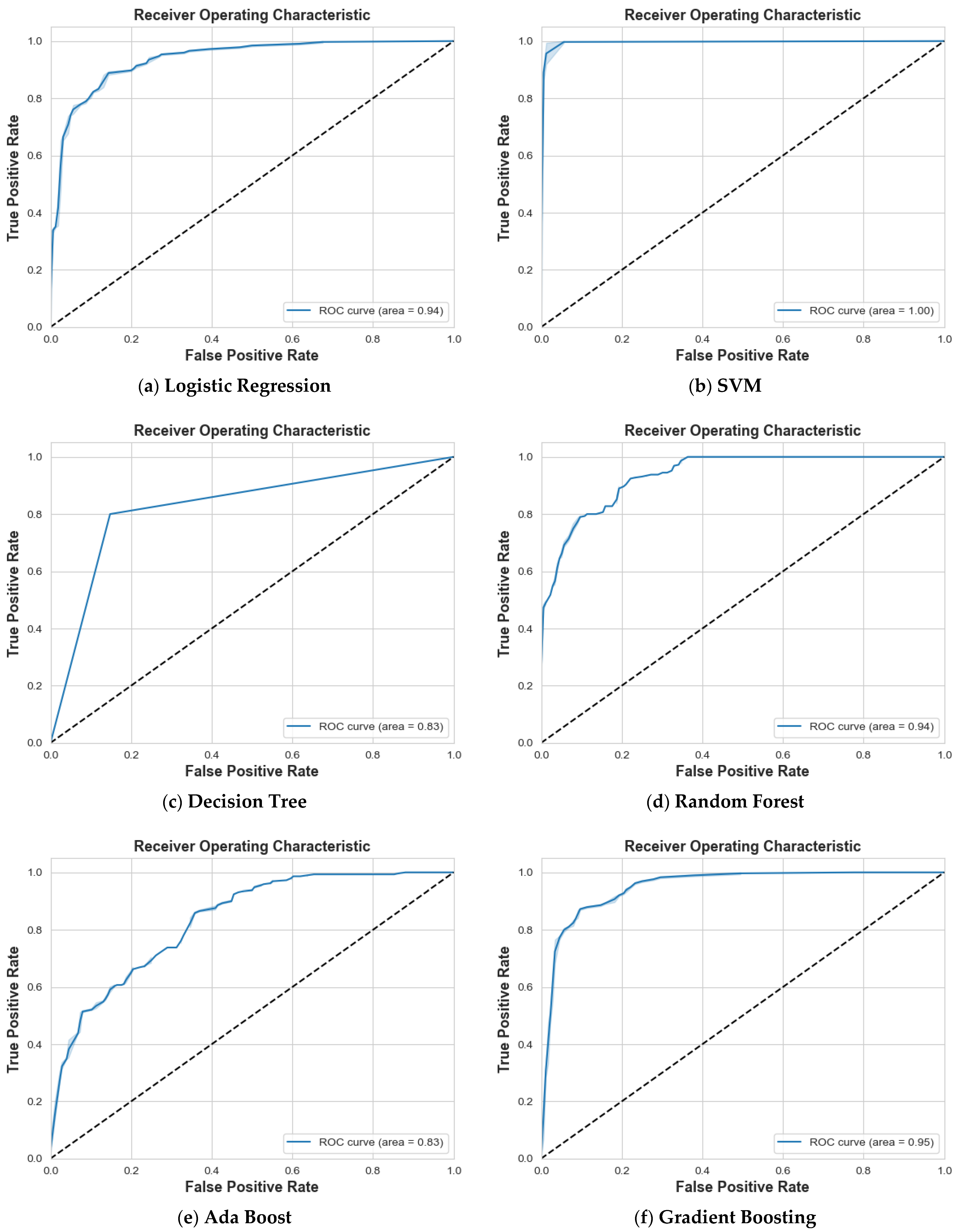
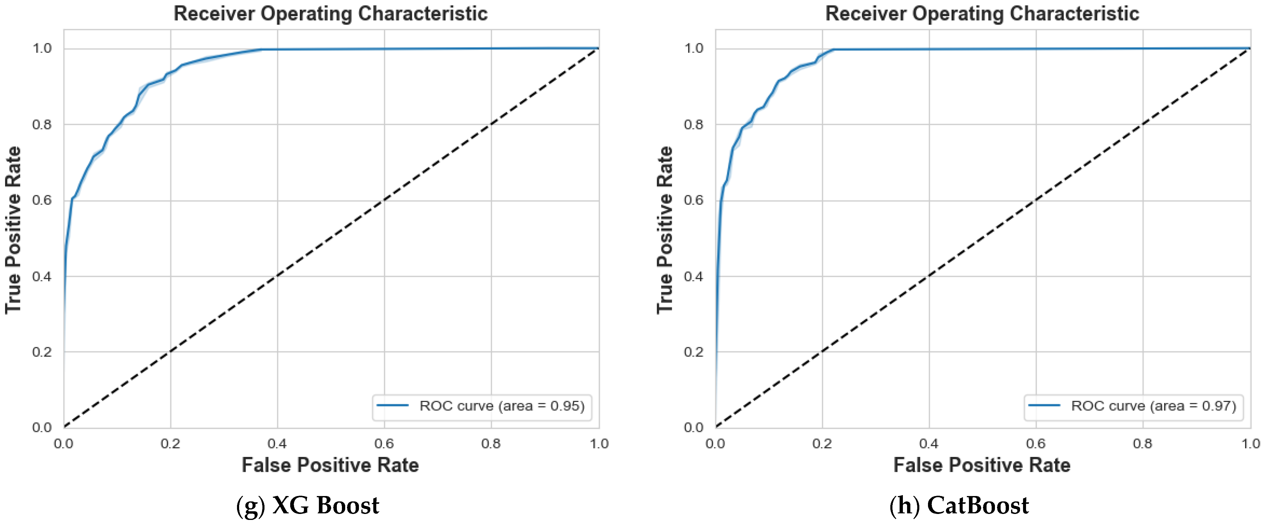
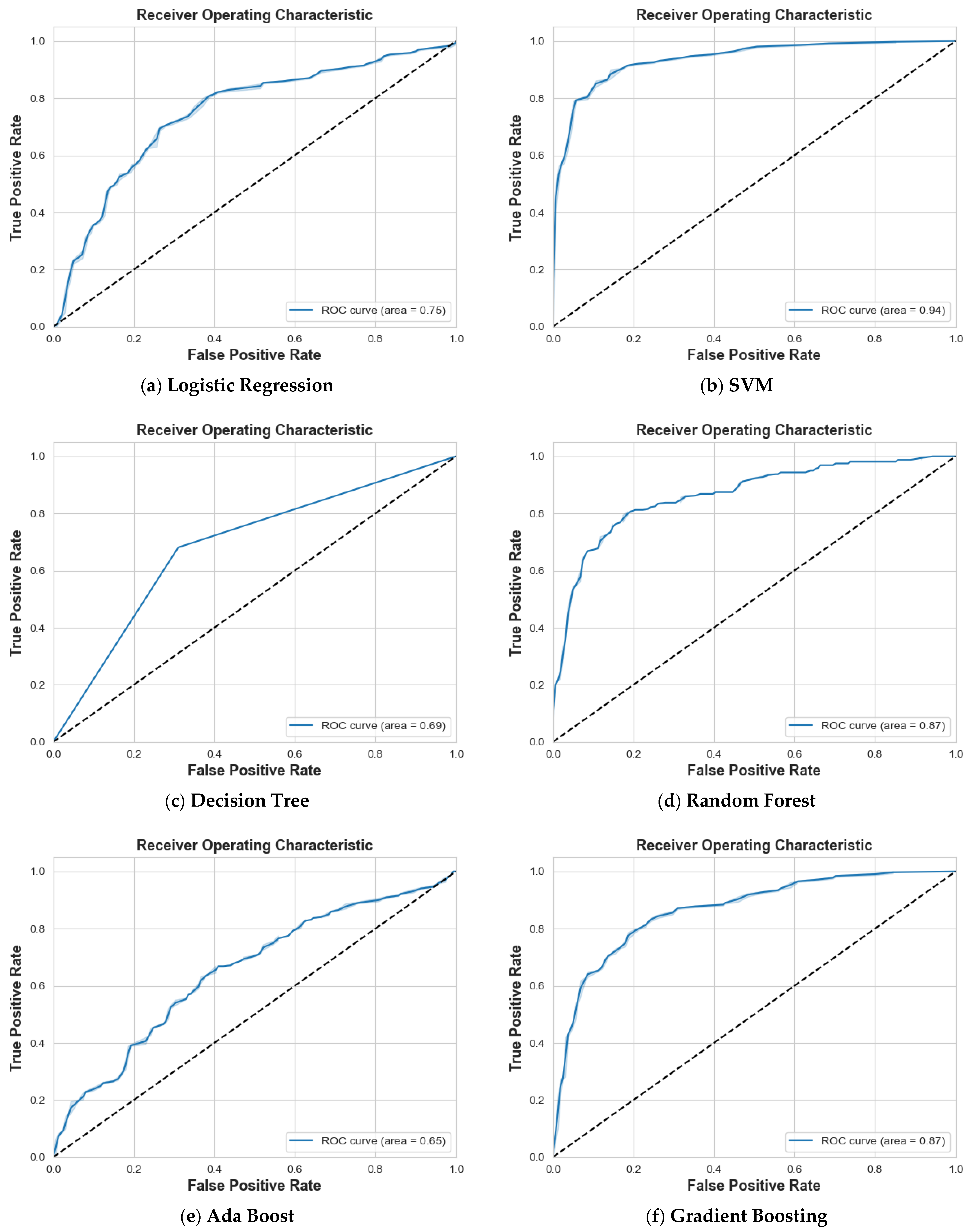
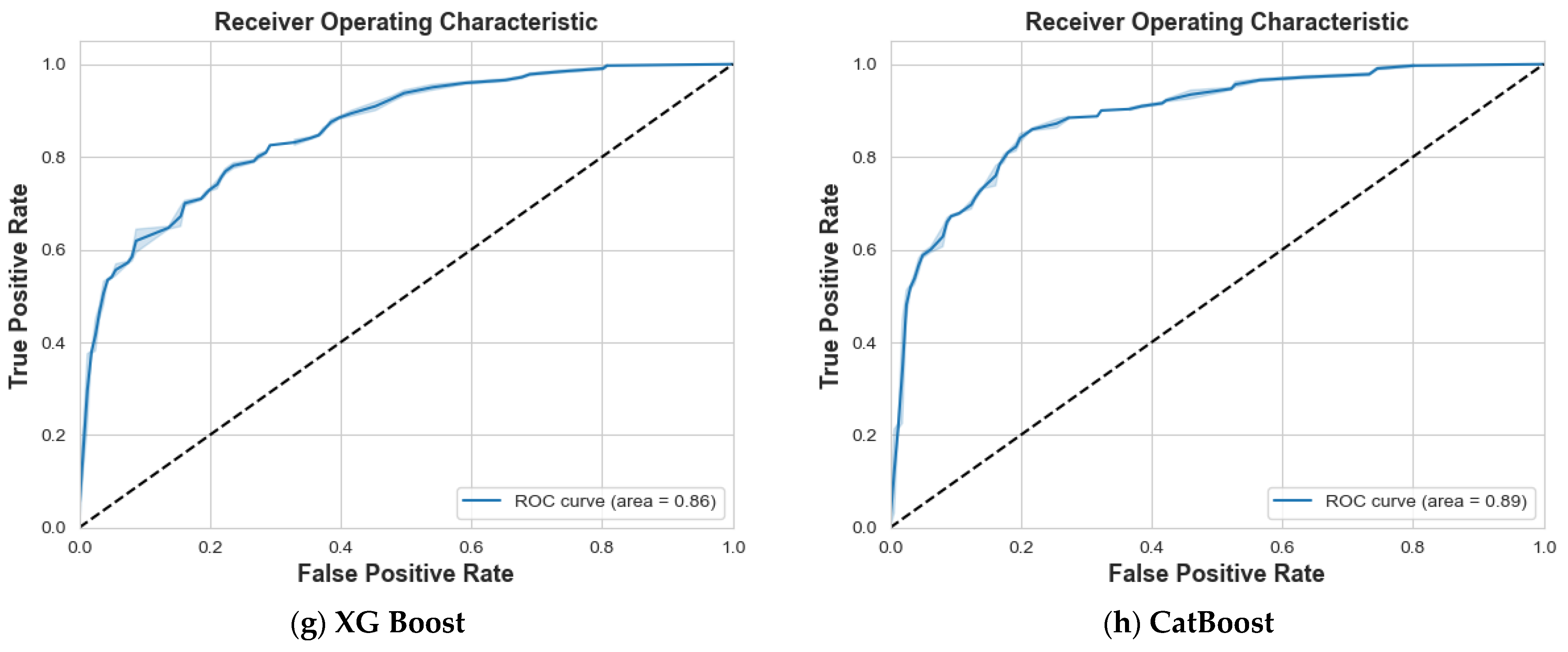
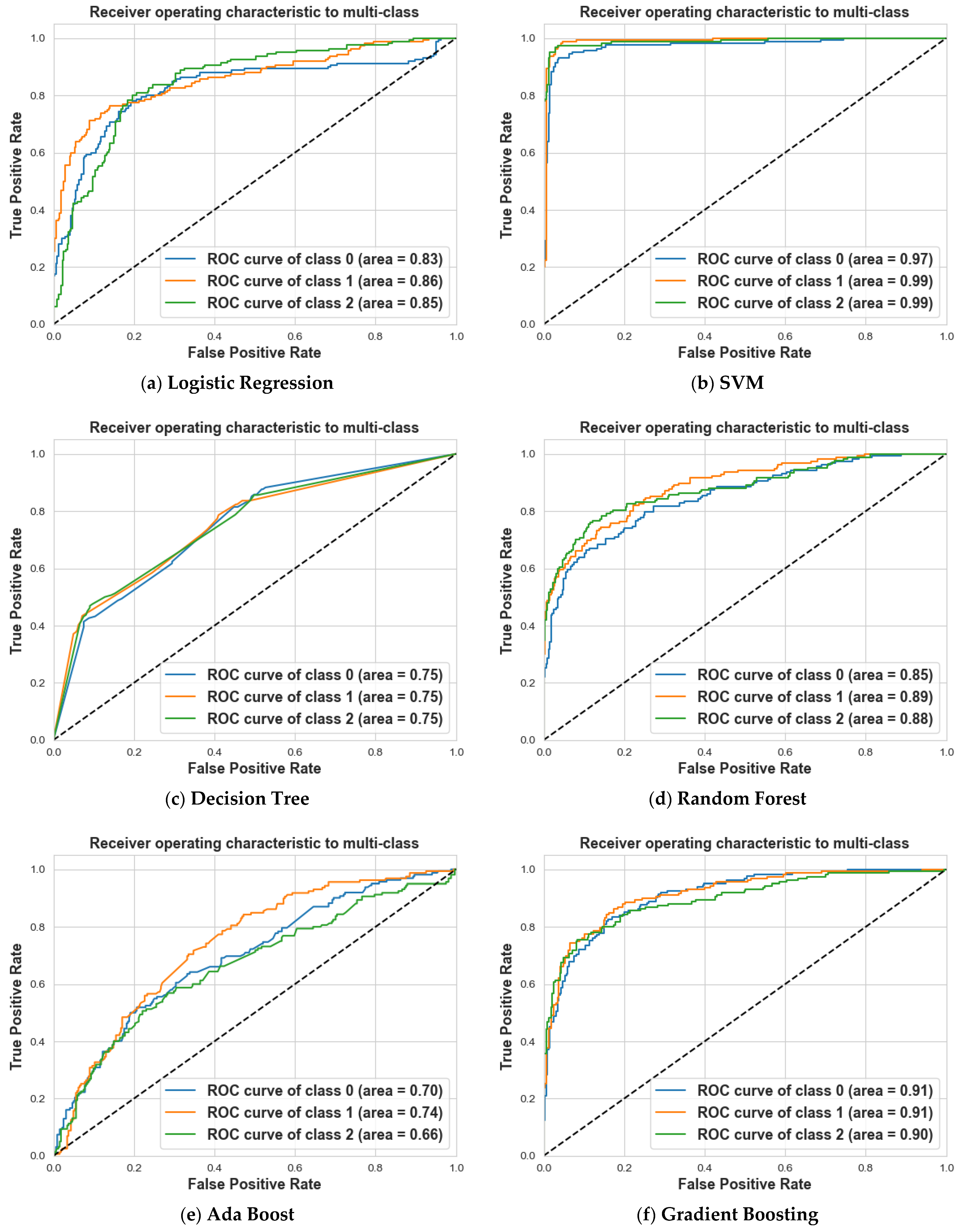
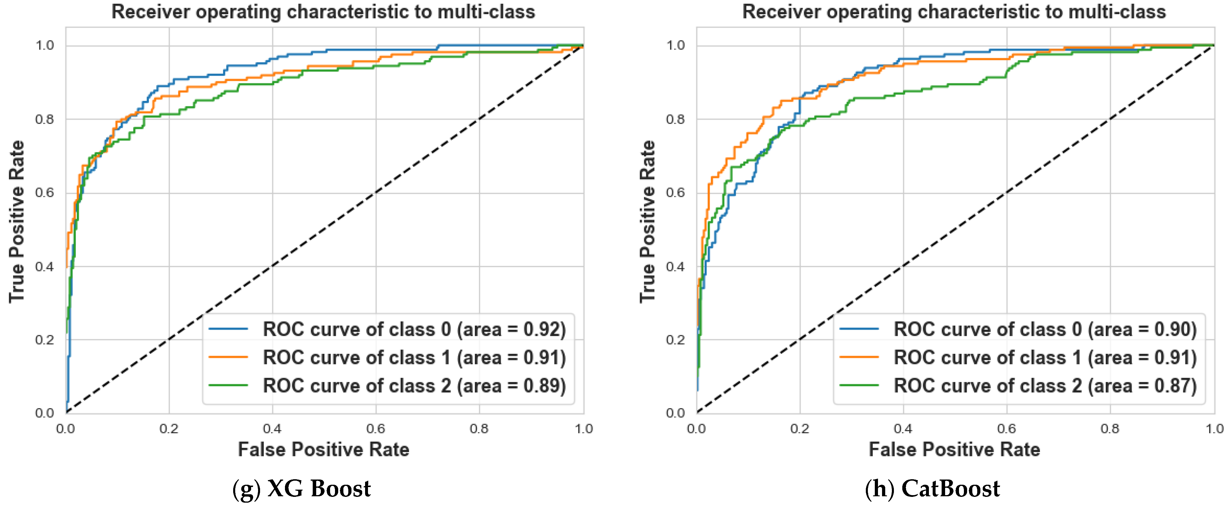
As shown in Table 4, eight MLAs were tested to discriminate a tumor from non-tumor cases. CatBoost and SVM showed exceptional accuracy, precision, recall, and F1 scores, with SVM achieving 98% accuracy and CatBoost 90%. As shown in Figure 9, the ROC analysis supported these findings, with SVM achieving a perfect AUC of 1.0 and CatBoost securing a strong AUC of 0.97, as shown in Figure 9b,h. LR, GB, XG Boost, and RF show decent performance with AUC values ranging from 0.94 to 0.95, as shown in Figure 9a,d,f,g. DT and Ada Boost achieve an AUC of 0.83, as shown in Figure 9c,e.
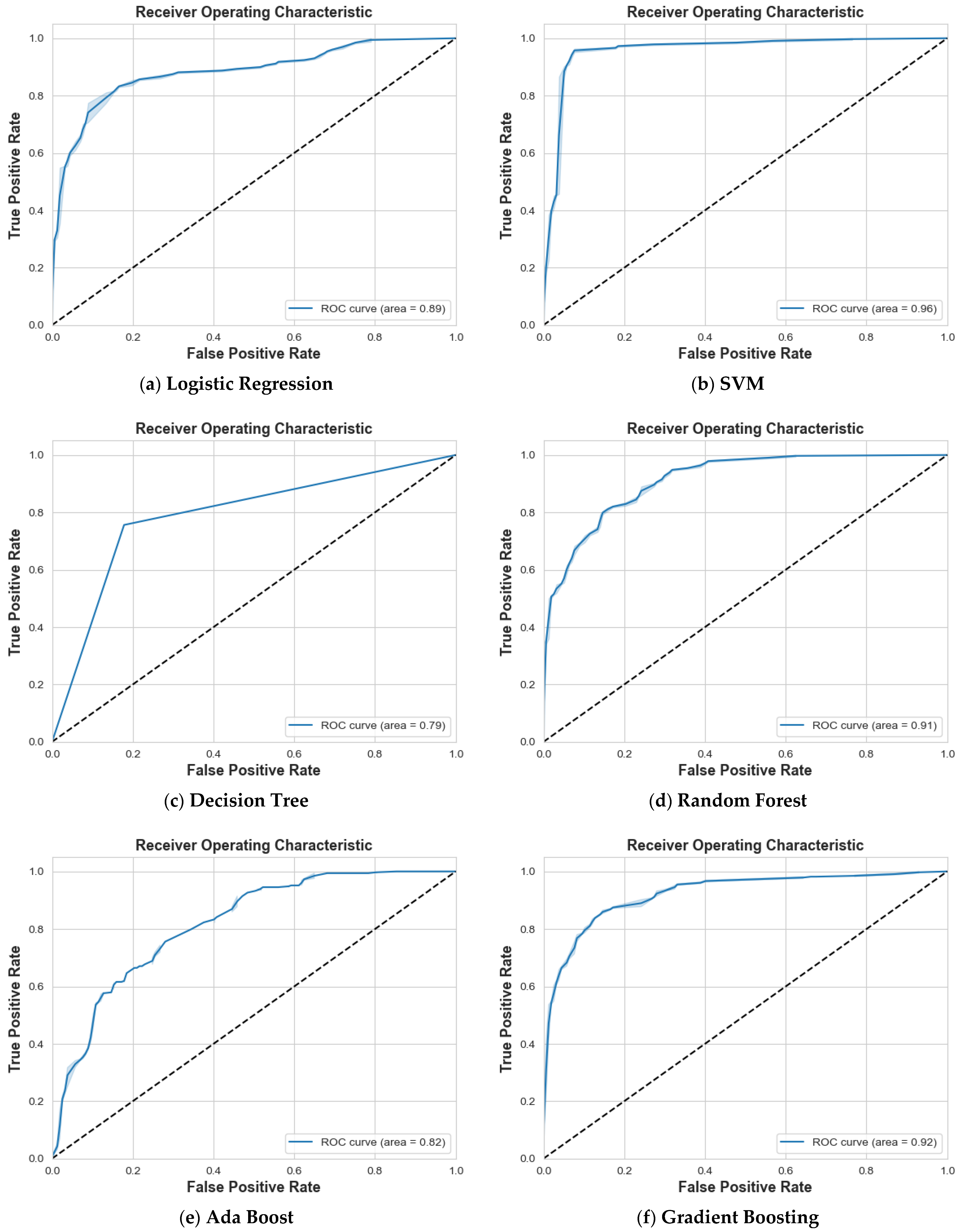
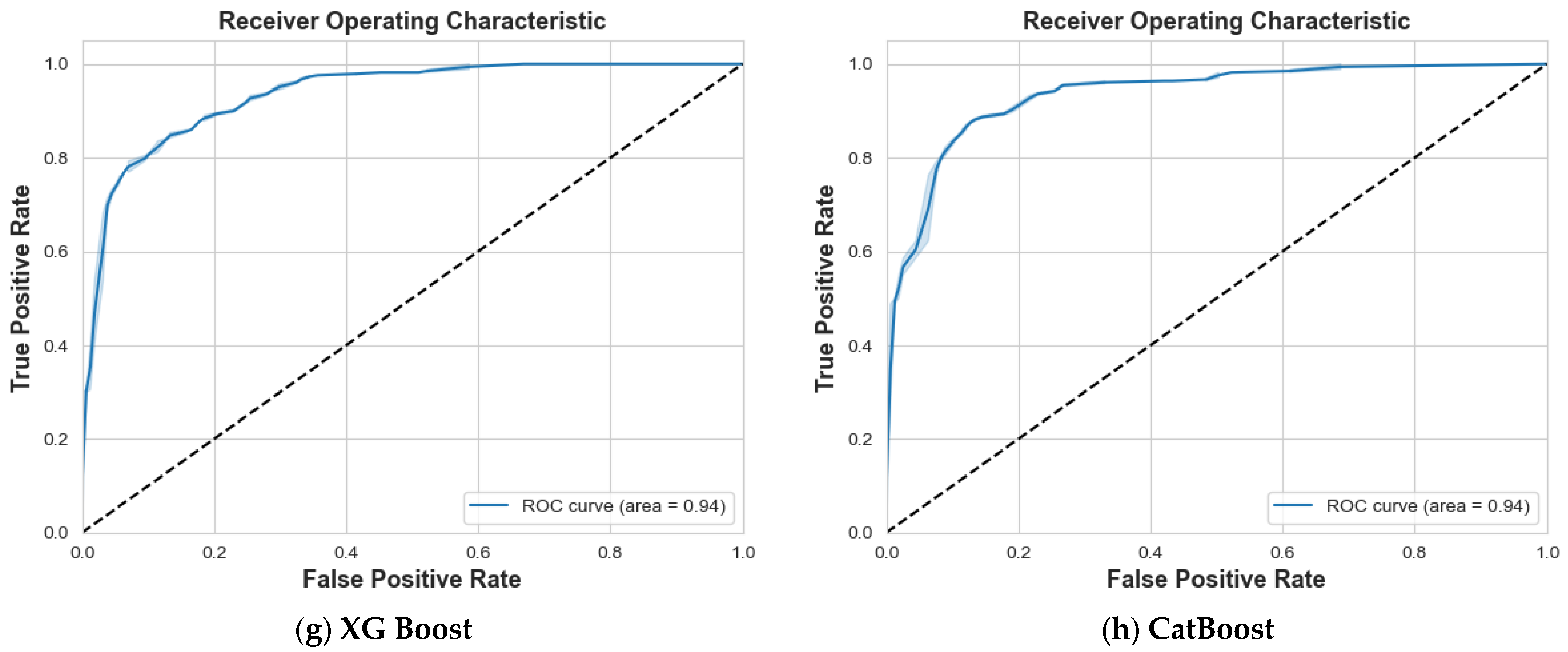
Table 5 illustrates a similar pattern with HV S 11 , where SVM performs better. As can be seen in Figure 10b, this algorithm has an accuracy score of 94% with an AUC of 0.96. Other algorithms that have accuracy scores between 73% and 87% with AUC in Figure 10a,c–g include DT, RF, Ada Boost, GB, XG Boost, and CatBoost.
Table 6’s HH S 21 displays a slightly different pattern. With an accuracy of 86% and an AUC of 0.94, as in Figure 11b, SVM leads in this case. GB and CatBoosting are next with 0.87 and 0.89 of AUC, as in Figure 11d,f,h. However, as shown in Figure 11a,c–e,g, LR, DT, RF, Ada Boost, and XG Boost find it difficult to keep up, with accuracy scores of 68%, 69%, 79%, 63%, and 77%, respectively, and an AUC ranging from 0.65 to 0.86.
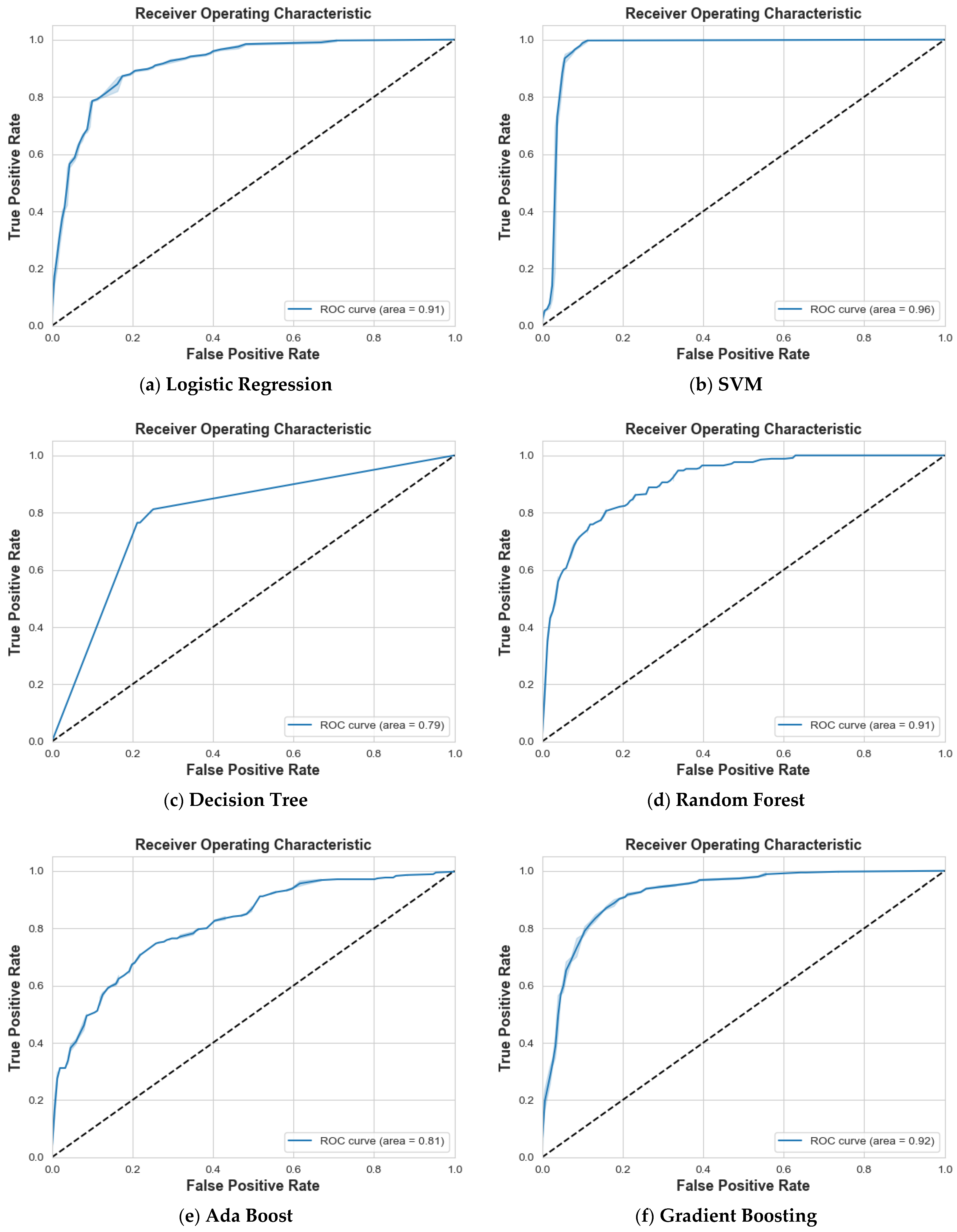
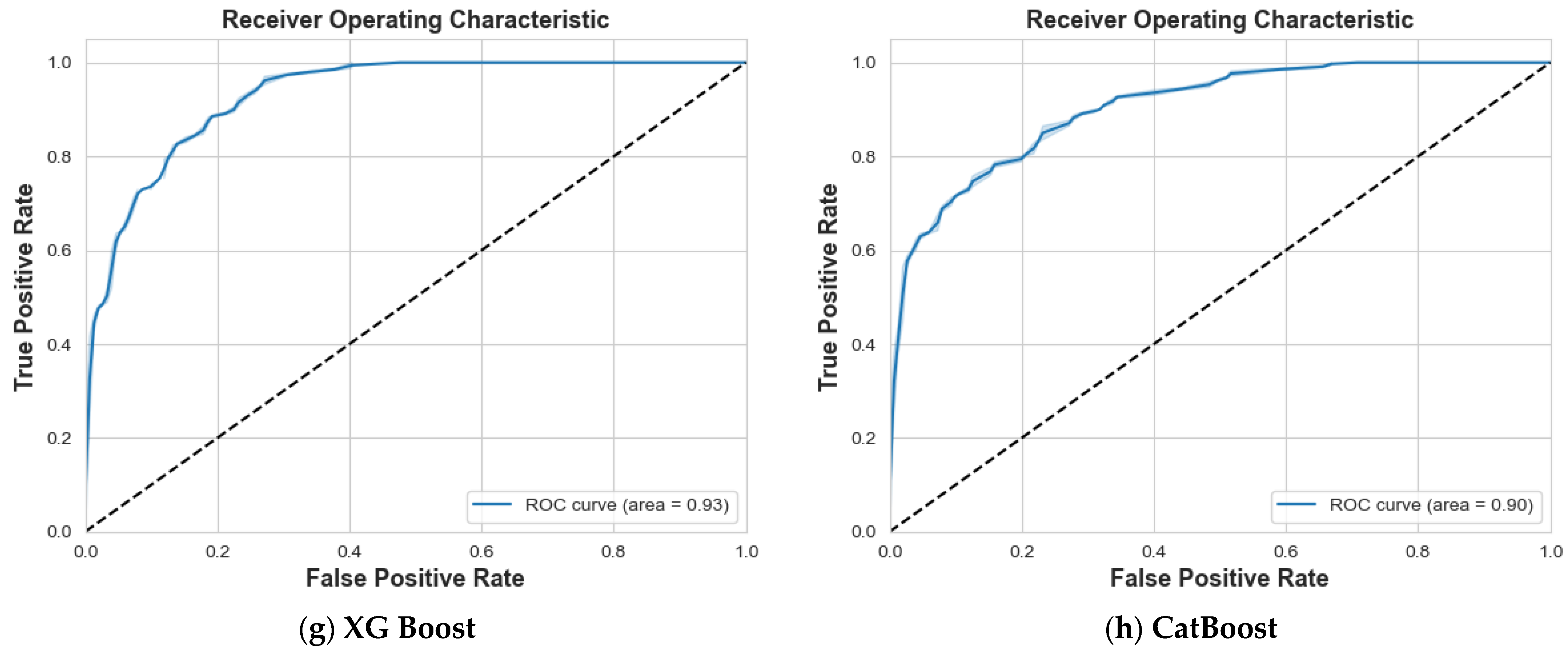
Lastly, the HV S 21 in Table 7 shows that SVM dominates the accuracy scores with 94% and 0.96 of AUC, as shown in Figure 12b. With an AUC of 0.91, LR performs fairly well, as seen in Figure 12a. As demonstrated in Figure 12c–h, in comparison, the accuracy of DT, RF, Ada Boost, GB, XG Boost, and CatBoost is lower and has a good range of AUC between 0.79 and 0.93.

4.2. Scenario 2: One, Two, and No Tumors

In the multi-class scenario, we used the ROC curve to evaluate the performance of each algorithm on the three classes (0, 1, and 2). Due to the limitations of the ROC curve in handling multiple classes, we plotted the ROC curves for each class separately, allowing for a more nuanced understanding of each algorithm’s performance. We used these metrics to compare the performance of the following algorithms: LR, SVM, DT, RF, Ada Boost, GBM, XG Boost, and CatBoost.
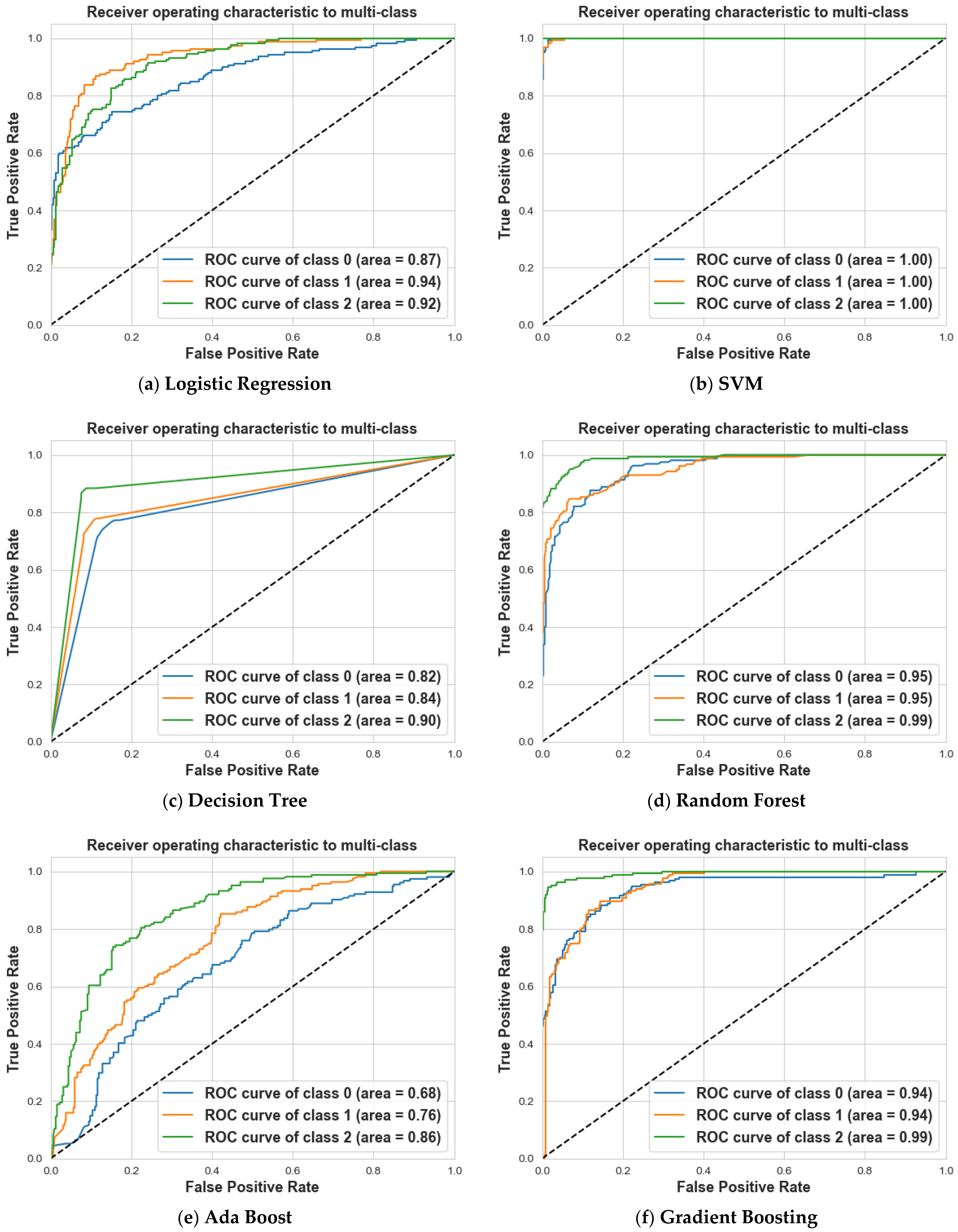
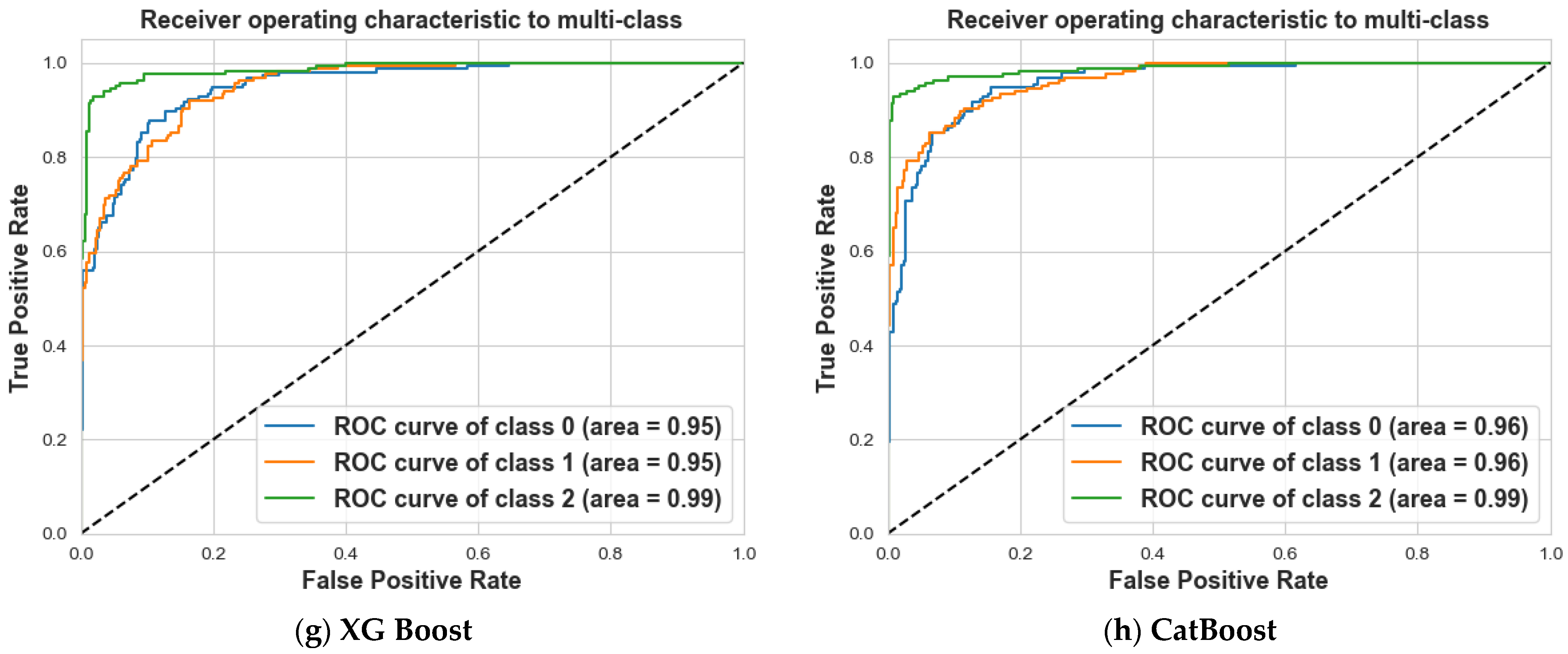
The eight MLA performance indicators, as presented in Table 8 for HH S 11 , reveal key insights. Figure 13b shows that SVM is the best performer, achieving an impressive 99% accuracy and an AUC of 1 across three classes. RF, GB, XG Boost, and CatBoost also perform well, with accuracy scores ranging from 85% to 88% and AUC values between 0.94 and 1, as depicted in Figure 12d,f–h. On the other hand, Figure 12c,e and Figure 13a illustrate that LR, DT, and Ada Boost struggle comparatively, with accuracy scores of 76%, 79%, and 58%, respectively, and lower AUC values in most classes.
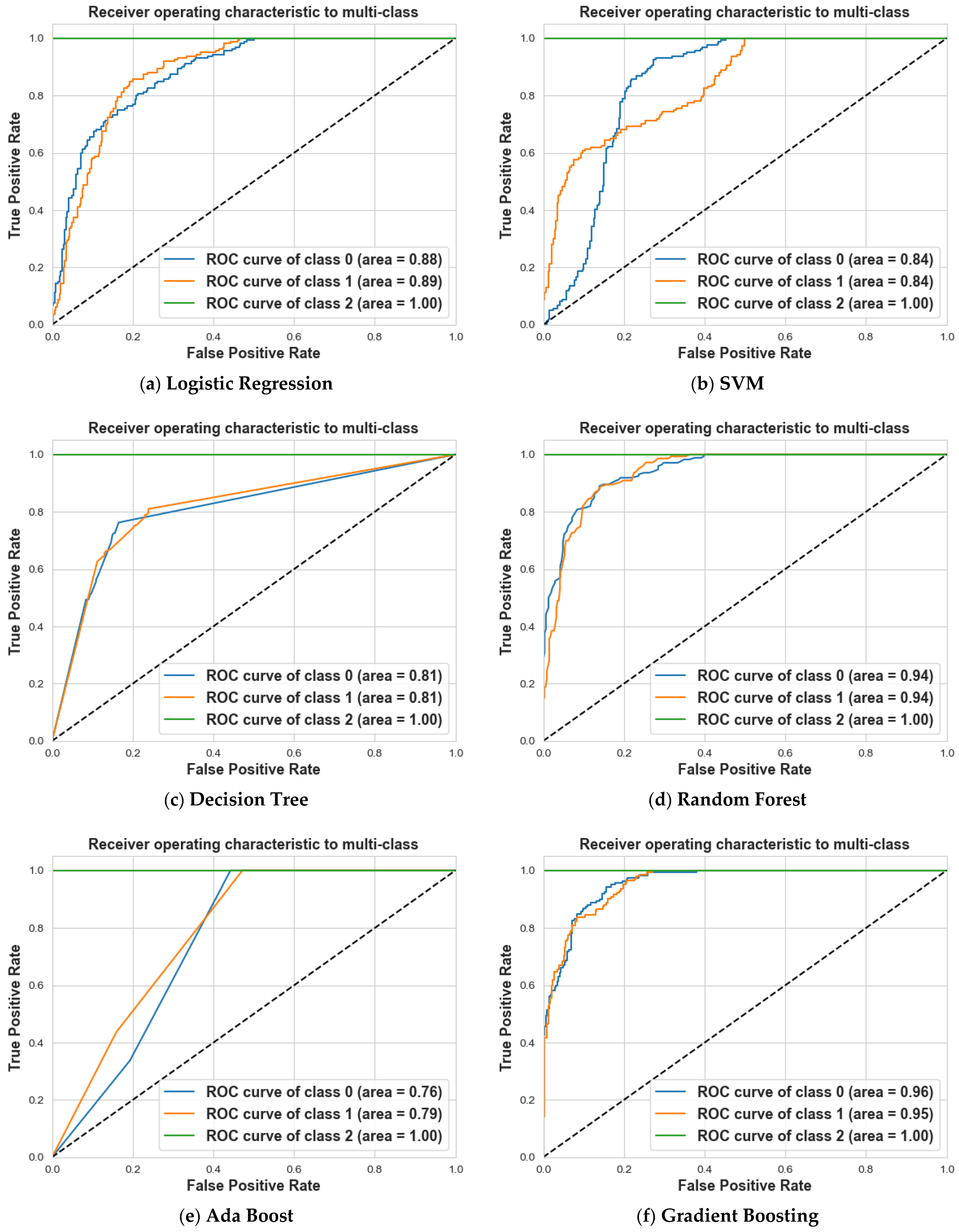
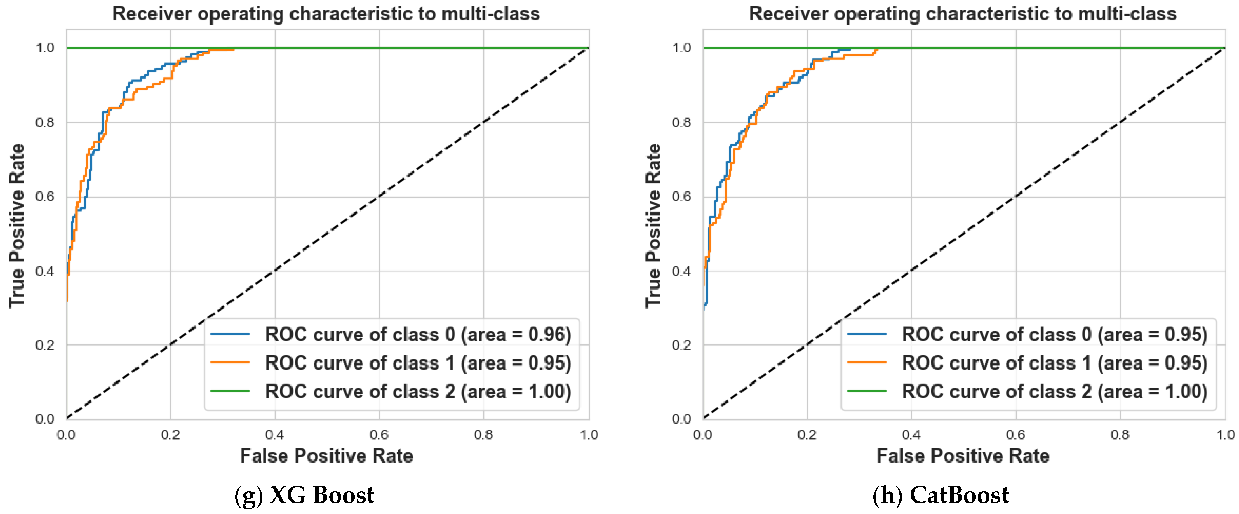
A slightly different pattern can be seen in HH S 21 for Scenario 2 in Table 9, where three algorithms with an AUC between 0.94 and 1.0 are used. RF, GB, and XG Boost take the lead with accuracy scores of 88%, as shown in Figure 14d,f,g. As seen in Figure 14h, CatBoost comes a close second with an accuracy score of 87% with 0.95 and 1.0 of AUC for three classes. Figure 14a–c,e shows that LR, SVM, DT, and Ada Boost lag behind with a low AUC in most classes.
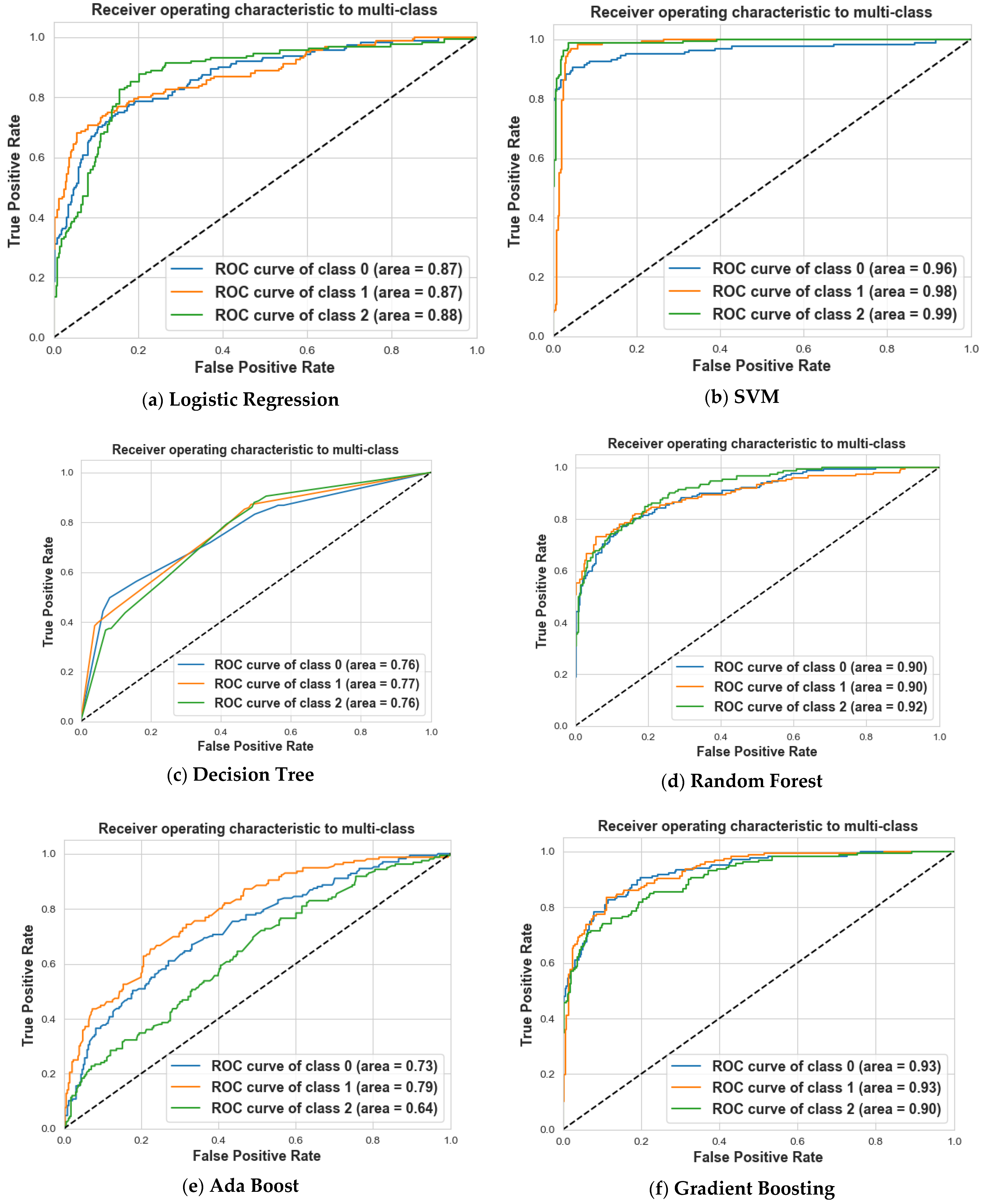
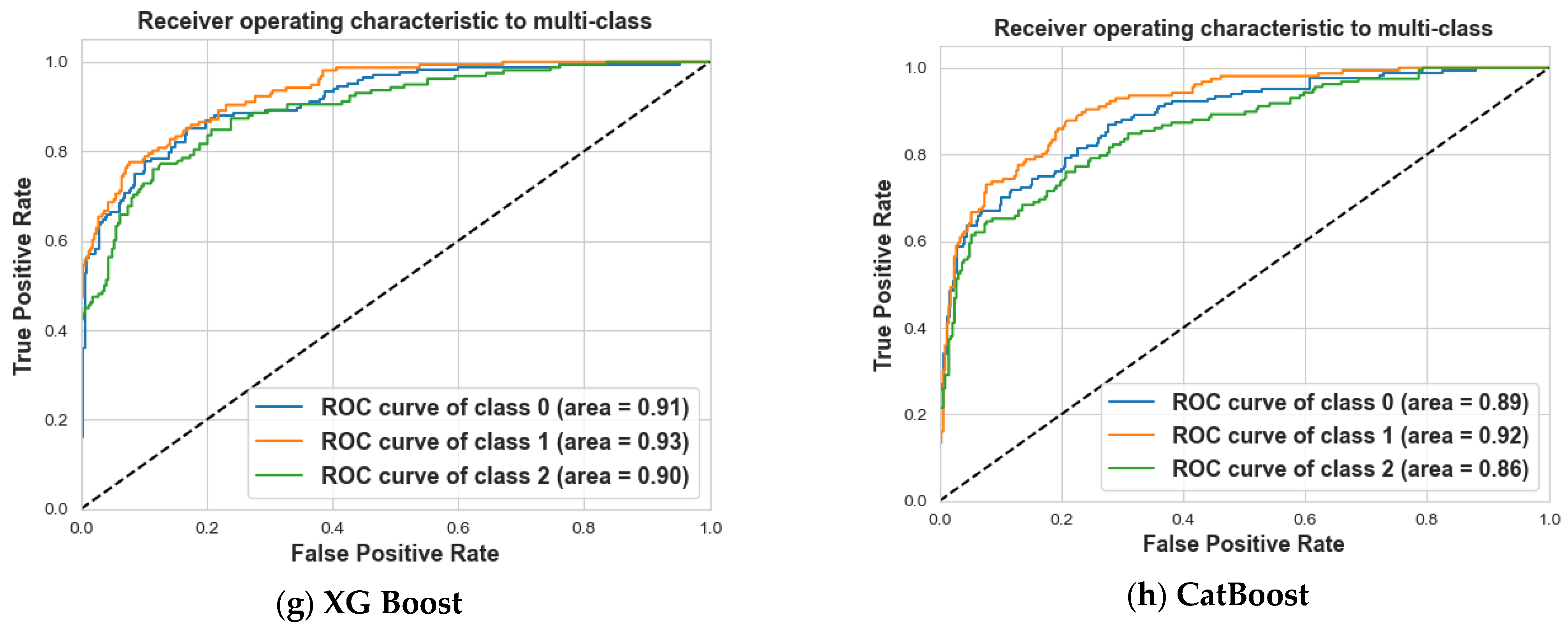
Similar results can be seen in Table 10 for HV S 11 , where SVM dominates the accuracy with 93% and AUC values of 0.96, 0.98, and 0.99 for the three classes, as shown in Figure 15b. Low accuracy is followed by LR, DT, RF, Ada Boost, GB, XG Boost, and CatBoost. As can be seen in Figure 15a,f–h, LR, GB, XG Boost, and CatBoost perform well for AUCs, while DT and Ada Boost lag behind for low AUCs, as can be seen in Figure 15c,d.
The HV S 21 results for Scenario 2 are shown in Table 11, and as Figure 16b shows, SVM achieves the highest accuracy score of 92% with a narrow range of AUC values. In comparison, the accuracy scores of the other algorithms range from 53% to 78%, indicating relatively low performance. In particular, as shown in Figure 16e–h, the ensemble algorithms—with the exception of AD—perform robustly with converging AUC values. Figure 16a,b,d show that LR, DT, and AD now have lower AUC values.
Looking at the results of our extensive research, a few important findings stand out. Firstly, SVMs demonstrated superior performance in identifying BC, consistently excelling in both scenarios, as shown in Figure 17a,b for Scenario 1 and Scenario 2. GB, XG Boost, and CatBoost also perform admirably, suggesting that they could be useful alternatives.
This comparison illustrates the superior performance of RF and XGBoost over SVM for the given datasets in terms of accuracy.
It is interesting to note that HV configuration generally performs worse than HH configuration. Based on these results, we recommend the use of dataset S 11 with its HH antenna configuration, which demonstrates optimal performance in our study.
Finally, based on the results mentioned above, we can conclude that LR is a robust algorithm for binary classification tasks like BC detection due to its ease of interpretability, fast training times, and lower computational requirements. However, its linear assumption and sensitivity to feature scaling can limit its effectiveness. SVM is a powerful MLA with high accuracy, effective handling of high-dimensional data, and clear class separation, but it can be resource-intensive and struggle with noisy data, particularly in BC detection tasks with moderate dataset sizes and complex feature spaces. DTs are a versatile classification and regression method, especially useful in BC detection due to their ability to handle non-linear relationships, minimal data pre-processing, and robustness to outliers. However, they can become computationally burdensome. RF is an effective technique for detecting BC because of its high accuracy, resilience to overfitting, and ability to work well with large datasets. Even with these drawbacks, RF remains useful and adaptable for tasks involving predictive modeling. Ada Boost is a versatile MLA for BC detection, enhancing weak learners’ performance and achieving high accuracy. However, it is sensitive to noisy data, requires hyperparameter tuning, and can be computationally intensive. GBM is a versatile algorithm for BC detection, capable of handling complex relationships and missing data. Despite its computational complexity, hyperparameter tuning requirements, and potential for overfitting, GBM remains a preferred choice for predictive modeling tasks. XG Boost is a robust MLA for BC detection despite its computational complexity, hyperparameter tuning, and interpretability issues. Despite these challenges, it remains a top choice for predictive modeling tasks. CatBoost is a robust ML tool for complex datasets like breast cancer detection, excelling in handling categorical features, achieving high accuracy, and preventing overfitting. Despite its computational complexity, need for fine-tuning, and longer training times, it remains effective and versatile. Table 12 provides a summary of various ML models, comparing them across several dimensions such as time complexity, problem type, and whether they are parametric or non-parametric models.

5. Conclusions

This paper presents a novel and innovative system for the early detection of BC using the pre-processed balanced dataset. By using a dual-polarization sensor-based wearable textile bra-tenna system together with ML, the system is able to effectively detect tumors as small as 10 mm. Eight distinct ML techniques were applied to the dataset and the performance of the system was analyzed in two scenarios. We trained each algorithm on 80% of the dataset and evaluated its performance on the remaining 20% test set. The results showed that the proposed system achieved excellent performance, with an accuracy of over 90% in both scenarios. This high level of accuracy surpasses that of existing methods and highlights the potential of microwave detection as a valuable tool for BC diagnosis.

Author Contributions

Conceptualization, A.H.E. and A.S.A.E.-H.; methodology, A.H.E. and N.F.F.A.; software validation, A.S.A.E.-H. and A.H.E.; formal analysis, N.F.F.A. and M.A.Y.; investigation, A.S.A.E.-H. and A.H.E.; writing—original draft preparation, A.H.E. and M.A.Y.; writing—review and editing, A.H.E.; visualization, A.S.A.E.-H. and N.F.F.A.; supervision, N.F.F.A. All authors have read and agreed to the published version of the manuscript.

Funding

This research received no external funding.

Informed Consent Statement

Not applicable.

Data Availability Statement

The raw data supporting the conclusions of this article will be made available by the authors upon request.

Acknowledgments

All authors would like to thank the Electronics Research Institute for offering the use of the institute’s laboratories and facilitating the work until its completion.

Conflicts of Interest

The authors declare no conflicts of interest.

References

  1. Tayel, M.; Abouelnaga, T.; Elnagar, A.H. Pencil Beam Grid Antenna Array for Hyperthermia Breast Cancer Treatment System. Circuits Syst. 2017, 8, 122–133. [Google Scholar] [CrossRef]
  2. Wang, L. Microwave Imaging and Sensing Techniques for Breast Cancer Detection. Micromachines 2023, 14, 1462. [Google Scholar] [CrossRef] [PubMed]
  3. Sarker, I.H. Ai-driven cyber security: An overview, security intelligence modeling and research directions. SN Comput. Sci. 2021, 2, 173. [Google Scholar] [CrossRef]
  4. Sarker, I.H.; Hoque, M.M. Mobile data science and intelligent apps: Concepts, AI-based modeling and research directions. Mob. Netw. Appl. 2021, 26, 285–303. [Google Scholar] [CrossRef]
  5. Sarker, I.H.; Kayes, A.S.M.; Badsha, S.; Alqahtani, H.; Watters, P.; Ng, A. Cybersecurity data science: An overview from machine learning perspective. J. Big Data 2020, 7, 41. [Google Scholar] [CrossRef]
  6. Mohammed, M.; Khan, M.B. Machine Learning: Algorithms and Applications; CRC Press: Boca Raton, FL, USA, 2016; ISBN 978-1-4987-0538-7. [Google Scholar] [CrossRef]
  7. Han, J.; Kamber, M. Data Mining: Concepts and Techniques; Elsevier: Amsterdam, The Netherlands, 2011. [Google Scholar]
  8. Witten, I.H.; Frank, E. Data Mining Practical machine learning tools and techniques. Morgan Kaufmann 2006, 2, 1–2. [Google Scholar]
  9. Sarker, I.H.; Watters, P. Effectiveness analysis of machine learning classification models for predicting personalized con text-aware smartphone usage. J. Big Data 2019, 6, 57. [Google Scholar] [CrossRef]
  10. Alazzam, B.; Mansour, M.; Hammam, H. Machine Learning of Medical Applications Involving Complicated Proteins and Genetic Measurements. Comput. Intell. Neurosci. 2023, 2023, 9839162. [Google Scholar] [CrossRef]
  11. An, Q.; Rahman, S. A Comprehensive Review on Machine Learning in Healthcare Industry: Classification, Restrictions, Opportunities and Challenges. Sensors 2023, 23, 4178. [Google Scholar] [CrossRef]
  12. Raza, A.; Ayub, H.; Khan, J.A.; Ahmad, I.; Salama, A.S.; Daradkeh, Y.I.; Javeed, D.; Ur Rehman, A.; Hamam, H. A Hybrid Deep Learning-Based Approach for Brain Tumor Classification. Electronics 2022, 11, 1146. [Google Scholar] [CrossRef]
  13. Nanmaran, R.; Srimathi, S.; Yamuna, G.; Thanigaivel, S.; Vickram, A.S.; Priya, A.K.; Karthick, A.; Karpagam, J.; Mohanavel, V.; Muhibbullah, M. Investigating the Role of Image Fusion in Brain Tumor Classification Models Based on Machine Learning Algorithm for Personalized Medicine. Comput. Math. Methods Med. 2022, 2022, 7137524. [Google Scholar] [CrossRef] [PubMed]
  14. Moslehi, S.; Rabiei, N.; Soltanian, A.R.; Mamani, M. Application of Machine Learning Models Based on Decision Trees in Classifying the Factors Affecting Mortality of COVID-19 Patients in Hamadan, Iran. BMC Med. Inform. Decis. Mak. 2022, 22, 192. [Google Scholar] [CrossRef] [PubMed]
  15. Begum, A.; Dhilip Kumar, V.; Asghar, J.; Hemalatha, D.; Arulkumaran, G. A Combined Deep CNN: LSTM with a Random Forest Approach for Breast Cancer Diagnosis. Complexity 2022, 2022, 9299621. [Google Scholar] [CrossRef]
  16. Lenhof, K.; Eckhart, L.; Gerstner, N.; Kehl, T.; Lenhof, H.-P. Simultaneous Regression and Classification for Drug Sensitivity Prediction Using an Advanced Random Forest Method. Sci. Rep. 2022, 12, 13458. [Google Scholar] [CrossRef] [PubMed]
  17. Friedman, J.H. Greedy Function Approximation: A Gradient Boosting Machine. Ann. Stat. 2001, 29, 1189–1232. [Google Scholar] [CrossRef]
  18. Wei, S.; Wu, Z. The Application of Wearable Sensors and Machine Learning Algorithms in Rehabilitation Training: A Systematic Review. Sensors 2023, 23, 7667. [Google Scholar] [CrossRef]
  19. Pedregosa, F.; Varoquaux, G.; Gramfort, A.; Michel, V.; Thirion, B.; Grisel, O.; Blondel, M.; Prettenhofer, P.; Weiss, R.; Dubourg, V.; et al. Scikit-learn: Machine learning in python. J. Mach. Learn. Res. 2011, 12, 2825–2830. [Google Scholar]
  20. Abd El-Hameed, A.S.; Elsheakh, D.M.; Elashry, G.M.; Abdallah, E.A. A comparative Study of Narrow/Ultra-wideband Micro-wave Sensors for Continuous Monitoring of Vital Signs and Lung Water Level. Sensors 2024, 24, 1658. [Google Scholar] [CrossRef]
  21. Alabrah, A.; Alkhamees, B.F.; Amin, F.; AlSalman, H.; Choi, G.S. Breast Breast Cancer Detection and Prevention Using Machine Learning. Diagnostics 2023, 13, 3113. [Google Scholar]
  22. Soumya, A.; Krishna Mohan, C.; Cenkeramaddi, L.R. Recent Advances in mmWave-Radar-Based Sensing, Its Applications, and Machine Learning Techniques: A Review. Sensors 2023, 23, 8901. [Google Scholar] [CrossRef]
  23. Sharma, S.; Aggarwal, A.; Choudhury, T. Breast Cancer Detection Using Machine Learning Algorithms. In Proceedings of the 2018 International Conference on Computational Techniques, Electronics and Mechanical Systems (CTEMS), Belgaum, India, 21–22 December 2018. [Google Scholar] [CrossRef]
  24. Reshan, M.S.A.; Amin, S.; Zeb, M.A.; Sulaiman, A.; Alshahrani, H.; Azar, A.T.; Shaikh, A. Enhancing Breast Cancer Detection and Classification Using Advanced Multi-Model Features and Ensemble Machine Learning Techniques. Life 2023, 13, 2093. [Google Scholar] [CrossRef] [PubMed]
  25. Syversen, A.; Dosis, A.; Jayne, D.; Zhang, Z. Wearable Sensors as a Preoperative Assessment Tool: A Review. Sensors 2024, 24, 482. [Google Scholar] [CrossRef] [PubMed]
  26. Michael, E.; Ma, H.; Li, H.; Qi, S. An Optimized Framework for Breast Cancer Classification Using Machine Learning. BioMed Res. Int. 2022, 2022, 8482022. [Google Scholar] [CrossRef] [PubMed]
  27. Dorogush, A.V.; Ershov, V.; Gulin, A. CatBoost: Gradient boosting with categorical features support. arXiv 2018, arXiv:1810.11363. [Google Scholar]
  28. Prokhorenkova, L.; Gusev, G.; Vorobev, A.; Dorogush, A.V.; Gulin, A. CatBoost: Unbiased boosting with categorical features. Adv. Neural Inf. Process. Syst. 2018, 31, 6639–6649. [Google Scholar]
  29. Vakaa, A.R.; Sonia, B.; Reddy, K.S. Breast cancer detection by leveraging Machine Learning. ICT Express 2020, 6, 320–324. [Google Scholar] [CrossRef]
  30. Rahayu, Y.; Waruwu, I. Early detection of breast cancer using ultra wide band slot antenna. SINERGI 2019, 23, 115. [Google Scholar] [CrossRef]
  31. Porter, E.; Bahrami, H.; Santorelli, A.; Gosselin, B.; Rusch, L.A.; Popovic, M. A Wearable Microwave Antenna Array for Time-Domain Breast Tumor Screening. IEEE Trans. Med. Imaging 2016, 35, 1501–1509. [Google Scholar] [CrossRef]
  32. Srinivasan, D.; Gopalakrishnan, M. Breast Cancer Detection Using Adaptable Textile Antenna Design. J. Med. Syst. 2019, 43, 177. [Google Scholar] [CrossRef]
  33. Moloney, B.M.; O’Loughlin, D.; Abd Elwahab, S.; Kerin, M.J. Breast Cancer Detection—A Synopsis of Conventional Modalities and the Potential Role of Microwave Imaging. Diagnostics 2020, 10, 103. [Google Scholar] [CrossRef]
  34. O’Loughlin, D.; O’Halloran, M.; Moloney, B.M.; Glavin, M.; Jones, E.; Elahi, M.A. Microwave Breast Imaging: Clinical Advances and Remaining Challenges. IEEE Trans. Biomed. Eng. 2018, 65, 2580–2590. [Google Scholar] [CrossRef] [PubMed]
  35. Arif, Z.A.; Abduljabbar, Z.H.; Taher, H.A.; Sallow, A.B.; Almufti, S.M. Exploring the Power of eXtreme Gradient Boosting Algorithm in Machine Learning: A Review. Acad. J. Nawroz Univ. 2023, 12, 320–334. [Google Scholar] [CrossRef]
  36. Agarap, A.F.M. On Breast Cancer Detection: An Application of Machine Learning Algorithms on the Wisconsin Diagnostic Dataset. In Proceedings of the ICMLSC 2018, 2nd International Conference on Machine Learning and Soft Computing, Phuoc Island, Vietnam, 2–4 February 2018; pp. 5–9. [Google Scholar]
  37. Gayathri, B.M.; Sumathi, C.P. Breast cancer diagnosis using machine learning algorithms—A survey. Int. J. Distrib. Parallel Syst. 2013, 4, 105–112. [Google Scholar]
  38. Bhise, S.; Bepari, S. Breast Cancer Detection using Machine Learning Techniques. Int. J. Eng. Res. Technol. 2021, 10, 2278-0181. [Google Scholar]
  39. Zhang, H.; Li, M.; Yang, F.; Xu, S.; Yin, Y.; Zhou, H. A feasibility study of 2-D microwave thorax imaging based on the supervised descent method. Electronics 2021, 10, 352. [Google Scholar] [CrossRef]
  40. Elsheakh, D.N.; Mohamed, R.A. Complete breast cancer detection and monitoring system by using microwave textile based antenna sensors. Biosensors 2023, 13, 87. [Google Scholar] [CrossRef]
  41. Mahesh, T.R.; Vinoth Kumar, V.; Muthukumaran, V.; Shashikala, H.K.; Swapna, B.; Guluwadi, S. Performance Analysis of XGBoost Ensemble Methods for Survivability with the Classification of Breast Cancer. J. Sens. 2022, 2022, 4649510. [Google Scholar] [CrossRef]
  42. Joshi, A.; Mehta, D.A. Comparative Analysis of Various Machine Learning Techniques for Diagnosis of Breast Cancer. Int. J. Emerg. Technol. 2017, 8, 522–526. [Google Scholar]
  43. Fatih, M. A Comparative Analysis of Breast Cancer Detection and Diagnosis Using Data Visualization and Machine Learning Applications. Healthcare 2020, 8, 111. [Google Scholar] [CrossRef]
  44. Asria, H.; Mousannifb, H.; Al Moatassime, H. Using Machine Learning Algorithms for Breast Cancer Risk Prediction and Diagnosis. Procedia Comput. Sci. 2016, 83, 1064–1069. [Google Scholar] [CrossRef]
  45. Bazazeh, D.; Shubair, R. Comparative Study of Machine Learning Algorithms for Breast Cancer Detection and Diagnosis. In Proceedings of the 2016 5th International Conference on Electronic Devices, Systems and Applications (ICEDSA), Ras Al Khaimah, United Arab Emirates, 6–8 December 2016. [Google Scholar] [CrossRef]
  46. Elnaggar, A.H.; Abd El-Hameed, A.S.; Yakout, M.A.; Areed, N.F. Development and comprehensive evaluation of a dual-port textile UWB MIMO antenna for biomedical use. Opt. Quantum Electron. 2024, 56, 1099. [Google Scholar] [CrossRef]
  47. Abd El-Hameed, A.S.; Wahab, M.G.; Elpeltagy, M. Quad-port UWB MIMO antenna based on LPF with vast rejection band. AEU-Int. J. Electron. Commun. 2021, 134, 153712. [Google Scholar] [CrossRef]
  48. Quintero, G.; Zurcher, J.-F.; Skrivervik, A.K. System fidelity factor: A new method for comparing UWB antennas. IEEE Antennas Wirel. Propag. Lett. 2011, 59, 2502–2512. [Google Scholar]
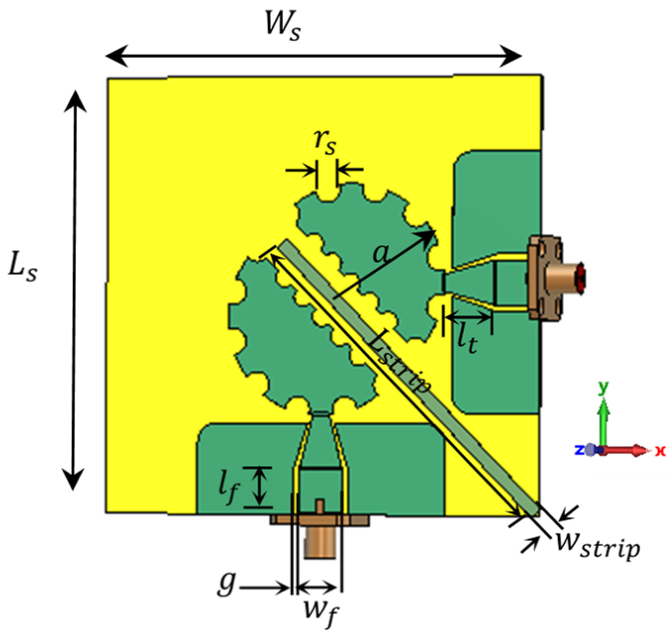
Figure 1. Geometric design of the proposed sensor.
Information 15 00467 g001
Figure 2. Fabricated prototype on conductive fabric and scattering parameters measurements. (a) Measurement setup. (b) Reflection coefficient. (c) Transmission coefficient.
Information 15 00467 g002
Figure 3. The proposed bra-tenna detection system.
Information 15 00467 g003
Figure 4. Proposed BC detection model.
Information 15 00467 g004
Figure 5. SVM classifier: (a) Data points are projected to calculate the distance to a hyperplane. (b) A diagram showing the maximum distance between SVMs to distinguish between various class divisions.
Information 15 00467 g005
Figure 6. Methodology of gathering datasets.
Information 15 00467 g006
Figure 7. The bra-tenna system analyzes distribution of the utilized dataset.
Information 15 00467 g007aInformation 15 00467 g007bInformation 15 00467 g007cInformation 15 00467 g007d
Figure 8. The bra-tenna system analyzes distribution of the utilized dataset.
Information 15 00467 g008aInformation 15 00467 g008bInformation 15 00467 g008cInformation 15 00467 g008d
Figure 9. ROC curve of various classifiers for HH S 11 .
Information 15 00467 g009aInformation 15 00467 g009b
Figure 10. ROC curve of various classifiers for HV: S 11 .
Information 15 00467 g010aInformation 15 00467 g010b
Figure 11. ROC curve of various classifiers for HH S 21 .
Information 15 00467 g011aInformation 15 00467 g011b
Figure 12. ROC curve of various classifiers for HV S 21 .
Information 15 00467 g012aInformation 15 00467 g012b
Figure 13. ROC curve of various classifiers for HH S 11 .
Information 15 00467 g013aInformation 15 00467 g013b
Figure 14. ROC curve of various classifiers for HH S 21 .
Information 15 00467 g014aInformation 15 00467 g014b
Figure 15. ROC curve of various classifiers for HV S 11 .
Information 15 00467 g015aInformation 15 00467 g015b
Figure 16. ROC curve of various classifiers for HV S 21 .
Information 15 00467 g016aInformation 15 00467 g016b
Figure 17. Highest accuracy for Scenario 1 and Scenario 2. (a) Performance variations of the SVM algorithm across different datasets, (b) Performance comparison of RF, GB, and XGBoost algorithms against the SVM algorithm.
Information 15 00467 g017
Table 1. Sample of original dataset BC.
Feature_1Feature_2Feature_3Feature_4Feature_5
−0.320734322071075–0.541588723659515i−0.323773860931396–0.549457371234894i−0.328166037797928–0.547743916511536i−0.330092638731003–0.545518636703491i−0.328741282224655–0.546375811100006i
−0.339545249938965–0.539299964904785i−0.345008134841919–0.54773360490799i−0.345800369977951–0.54529732465744i−0.34616020321846–0.542522668838501i−0.347417116165161–0.547296822071075i
Table 2. Sample of dataset breast cancer after pre-processing.
Feature_1Feature_2Feature_3Feature_4Feature_5
0.4236030.4232090.4294940.4331120.436930
0.4723820.4704310.4759640.4736920.475052
0.2518080.2543440.2494890.2483620.242685
0.4001510.3983280.4036050.409770.41290
0.2491650.2518670.2508150.239650.24348
Table 3. Pseudo-code for Scenario 1.
1. IMPORT LIBRARIES: numpy, pandas, sklearn.model_selection
2. DEFINE FILE PATHS: PATH_with, PATH_without
3. READ CSV FILES: df_with, df_without = read_csv(PATH_with, PATH_without)
4. CONVERT TO COMPLEX NUMBERS: df_with, df_without = convert_to_complex(df_with, df_without)
5. CALCULATE MAGNITUDES: df_with, df_without = calculate_magnitudes(df_with, df_without)
6. ADD TUMOR COLUMN: df_with[‘tumor’] = 1, df_without[‘tumor’] = 0
7. CONCATENATE DATAFRAMES: df = concatenate(df_with, df_without)
8. SHUFFLE ROWS: df = shuffle(df)
9. SPLIT DATA: train, test = split(df), test_size = 0.2
Table 4. Comparison of machine learning algorithms based on HH S 11 .
Class 0: Non-TumorClass 1: One Tumor
ModelsPrecisionRecallF1Precision RecallF1AccuracyAUC
Logistic Regression87%87%87%87%88%87%87%0.94
SVM97%99%98%99%97%98%98%1
Decision Tree84%85%85%82%80%81%83%0.83
Random Forest86%84%85%81%83%82%83%0.94
Ada Boost74%77%75%71%68%69%73%0.83
Gradient Boosting90%88%89%85%88%87%88%0.95
XG Boost87%86%87%84%85%84%86%0.95
CatBoost92%89%90%87%91%89%90%0.97
Table 5. Comparison of machine learning algorithms HV S 11 .
Class 0: Non-TumorClass 1: One Tumor
ModelsPrecisionRecallF1PrecisionRecallF1Accuracy AUC
Logistic Regression81%87%84%86%81%84%84%0.89
SVM95%92%94%93%96%94%94%0.96
Decision Tree76%82%79%82%76%78%79%0.79
Random Forest81%85%83%85%80%83%83%0.91
Ada Boost71%73%72%74%72%73%73%0.82
Gradient Boosting84%87%86%87%84%86%86%0.92
XG Boost85%83%84%84%86%85%85%0.94
CatBoost85%89%87%89%85%87%87%0.94
Table 6. Comparison of machine learning algorithms HH S 21 .
Class 0: Non-TumorClass 1: One Tumor
ModelsPrecision RecallF1Precision RecallF1Accuracy AUC
Logistic Regression60%78%68%78%60%68%68%0.75
SVM80%91%85%92%82%87%86%0.94
Decision Tree69%69%69%69%68%68%69%0.69
Random Forest81%77%79%78%81%80%79%0.87
Ada Boost63%61%62%62%64%63%63%0.65
Gradient Boosting79%81%80%81%79%80%80%0.87
XG Boost78%76%77%76%79%78%77%0.86
CatBoost83%80%82%81%84%82%82%0.89
Table 7. Comparison of machine learning algorithms HV S 21 .
Class 0: Non-TumorClass 1: One Tumor
ModelsPrecisionRecallF1Precision RecallF1Accuracy AUC
Logistic Regression87%82%84%83%88%85%85%0.91
SVM98%91%94%91%98%95%94%0.96
Decision Tree75%78%76%80%76%78%77%0.79
Random Forest80%81%81%83%82%82%81%0.91
Ada Boost72%72%72%75%75%75%74%0.81
Gradient Boosting84%85%85%87%86%86%83%0.92
XG Boost80%87%83%87%81%84%84%0.93
CatBoost77%80%79%82%79%80%79%0.90
Table 8. Comparison of machine learning algorithms HH S 11 .
Class 0: Non-Tumor Class 1: One Tumor Class 2: Two Tumors
ModelsPrec. RecallF1Prec. RecallF1Prec. RecallF1Accuracy
Logistic Regression85%66%75%70%87%78%75%74%74%76%
SVM97%99%98%99%97%98%100%100%100%99%
Decision Tree71%77%74%82%73%77%85%87%86%79%
Random Forest83%78%81%83%83%83%90%94%92%85%
Ada Boost52%53%52%58%52%55%65%70%67%58%
Gradient Boosting81%79%80%81%80%80%92%96%94%85%
XG Boost82%79%81%81%79%80%90%95%93%85%
CatBoost84%84%84%85%85%85%95%95%95%88%
Table 9. Comparison of machine learning algorithms HH S 21 .
Class 0: Non-Tumor Class 1: One Tumor Class 2: Two Tumors
ModelsPrec. RecallF1Prec. RecallF1Prec. RecallF1Accuracy
Logistic Regression67%76%71%72%63%67%100%100%100%80%
SVM58%94%71%83%31%45%100%100%100%75%
Decision Tree72%58%64%61%74%67%100%100%100%78%
Random Forest86%78%82%76%85%80%100%100%100%88%
Ada Boost57%66%61%53%44%48%100%100%100%72%
Gradient Boosting84%78%81%77%84%80%100%100%100%88%
XG Boost85%77%81%77%85%81%100%100%100%88%
CatBoost81%79%80%77%80%78%100%100%100%87%
Table 10. Comparison of machine learning algorithms for HV S 11 .
Class 0: Non-Tumor Class 1: One Tumor Class 2: Two Tumors
ModelsPrec. RecallF1Prec. RecallF1Prec. RecallF1Accuracy
Logistic Regression73%74%74%76%72%74%71%75%73%74%
SVM87%93%90%97%90%93%96%95%95%93%
Decision Tree52%61%56%54%57%55%66%50%57%56%
Random Forest73%67%70%75%72%73%72%80%76%73%
Ada Boost51%46%49%54%53%54%46%51%49%50%
Gradient Boosting73%78%75%79%77%78%79%76%77%77%
XG Boost76%80%78%77%79%78%80%72%76%77%
CatBoost71%74%72%75%75%75%74%70%72%73%
Table 11. Comparison of machine learning algorithms HV S 21 .
Class 0: Non-Tumor Class 1: One Tumor Class 2: Two Tumors
ModelsPrec. RecallF1Prec. RecallF1Prec. RecallF1Accuracy
Logistic Regression72%76%74%77%69%73%74%78%76%74%
SVM93%88%90%94%93%93%92%98%95%92%
Decision Tree95%56%60%48%77%59%68%37%48%57%
Random Forest79%74%77%82%71%76%69%84%76%76%
Ada Boost57%54%56%56%58%57%47%47%47%53%
Gradient Boosting77%83%80%83%77%80%75%74%75%78%
XG Boost75%80%77%81%78%79%76%73%75%77%
CatBoost71%74%72%75%77%76%71%66%69%72%
Table 12. Parameter of machine learning algorithms.
ParameterTime Complexity
(Training Phase)
Problem TypeModel Parameter
Models
LRn(O(d)) = O(nd)ClassificationParametric
SVMO( n 2 × d) or O( n 3 )Classification and regressionNon-parametric
DTO(m · n 2 )Classification and regressionNon-parametric
RFO(v × n log(n))Classification and regressionNon-parametric
Ada BoostO(Tf)Classification and regressionNon-parametric
GBMO(Td)Classification and regressionNon-parametric
XG BoostO(tdxlogn)Classification and regressionNon-parametric
CatBoostO(sn2)Classification and regressionNon-parametric
Disclaimer/Publisher’s Note: The statements, opinions and data contained in all publications are solely those of the individual author(s) and contributor(s) and not of MDPI and/or the editor(s). MDPI and/or the editor(s) disclaim responsibility for any injury to people or property resulting from any ideas, methods, instructions or products referred to in the content.