Article

A Collaborative Allocation Algorithm of Communicating, Caching and Computing Resources in Local Power Wireless Communication Network

1
State Key Laboratory of Networking and Switching Technology, Beijing University of Posts and Telecommunications, Beijing 100876, China
2
State Grid Ningxia Electric Power Co., Ltd., Yinchuan 750001, China
*
Authors to whom correspondence should be addressed.
Information 2024, 15(6), 309; https://doi.org/10.3390/info15060309
Submission received: 17 April 2024 / Revised: 19 May 2024 / Accepted: 22 May 2024 / Published: 27 May 2024
(This article belongs to the Special Issue Internet of Things and Cloud-Fog-Edge Computing)

Abstract

:
With the rapid development of new power systems, diverse new power services have imposed stricter requirements on network resources and performance. However, the traditional method of transmitting request data to the IoT management platform for unified processing suffers from large delays due to long transmission distances, making it difficult to meet the delay requirements of new power services. Therefore, to reduce the transmission delay, data transmission, storage and computation need to be performed locally. However, due to the limited resources of individual nodes in the local power wireless communication network, issues such as tight coupling between devices and resources and a lack of flexible allocation need to be addressed. The collaborative allocation of resources among multiple nodes in the local network is necessary to satisfy the multi-dimensional resource requirements of new power services. In response to the problems of limited node resources, inflexible resource allocation, and the high complexity of multi-dimensional resource allocation in local power wireless communication networks, this paper proposes a multi-objective joint optimization model for the collaborative allocation of communication, storage, and computing resources. This model utilizes the computational characteristics of communication resources to reduce the dimensionality of the objective function. Furthermore, a mouse swarm optimization algorithm based on multi-strategy improvements is proposed. The simulation results demonstrate that this method can effectively reduce the total system delay and improve the utilization of network resources.

1. Introduction

As an essential part of the new power system, the local power wireless communication network is responsible for carrying numerous new local power communication services, achieving the adaptation of different wireless communication protocols for terminals, and fulfilling the functions of power information perception and power data transmission. It serves as the data collection entrance for the new power system [1]. However, with the digitalization of the new power system, various new power services emerging in the power grid have brought massive data and diverse demands [2], imposing higher requirements on the service quality and processing capabilities of the network [3]. The traditional approach of centralized processing through the IoT management platform not only results in significant processing delays, making it difficult to meet business needs, but also puts tremendous pressure on the backbone communication network’s carrying capacity and the cloud server’s computing capabilities due to the transmission of massive data [4]. To meet the multi-dimensional resource and delay requirements of new power services and reduce transmission delays, it is necessary to allocate resources such as communication, storage and computing in the local communication network. However, in the local power communication network, on the one hand, due to the tight coupling of equipment and resources, resource allocation is not flexible enough. On the other hand, the limited resources of a single node in the network make it difficult to simultaneously satisfy the multi-dimensional resource requirements of new power services for communication, storage and computing. Therefore, the collaborative scheduling of communication, storage, and computing resources among nodes is required to make full use of the network resources of local nodes, improve the network service quality, and reduce the processing delay of service requests.
Currently, due to its high computational complexity, research on the collaborative allocation of multi-dimensional resources commonly involves separate calculations for service transmission paths and resource allocation decisions. This approach involves first calculating the transmission paths and then further determining the resource allocation decisions based on these pre-computed paths [5]. Another common solution method is to adopt a greedy strategy, transforming the problem into a solution that finds several local optimal values [6] or prioritizes different services based on their resource requirements or latency constraints, and applying different allocation strategies for different priorities [7,8]. The literature [7] combines multi-access edge computing technology and cloud computing technology to jointly process the computing, caching, communicating and control (4C) resources of multi-access edge computing servers. It formulates the joint 4C problem as an optimization problem targeting a linear combination of joint bandwidth resources and network latency. The original problem is transformed into an approximate upper-bound problem and solved using a block-wise continuous minimization upper-bound method, effectively reducing the network bandwidth resource consumption and network delay. The literature [9] considers the joint optimization problem of binary caching decisions, computing resources and bandwidth allocation in a multi-user caching-assisted mobile edge computing scenario aimed at minimizing the total energy consumption. It proposes an offline caching placement scheme based on deep learning, effectively reducing the system energy consumption. In [10], computing offloading, content caching and resource allocation strategies aimed at minimizing the total delay of computational tasks in mobile edge computing networks are investigated. It formulates this as a mixed-integer nonlinear programming problem and uses an improved branch-and-bound method to solve the asymmetric search tree. Additionally, an improved generalized bending decomposition method is applied to reduce the time complexity of the solution. There are also other methods for calculating resource allocation strategies [9,11,12,13,14,15,16,17].
Therefore, this paper proposes a collaborative allocation model for communicating, caching and computing resources in local power wireless communication network, along with a multi-objective joint optimization method for a collaborative allocation algorithm for communicating, caching and computing resources. The algorithm is based on a multi-strategy-improved RSO algorithm, which utilizes iterative chaotic mapping to improve the process of initializing the population. It also employs a mutation strategy based on the idea of differential evolution to enhance the iterative process used for individuals in the population. Furthermore, the control factors of RSO are nonlinearly optimized. The simulation results show that the proposed MRSO algorithm can reduce the total system cost and improve the utilization rate of network resources.
The rest of this paper is organized as follows. The collaborative allocation model for communicating, caching and computing resources is shown in Section 2. In Section 3, we provide details of the proposed MRSO algorithm. The simulation results are shown in Section 4 and the conclusions are discussed in Section 5.

2. Collaborative Allocation Model of Communicating, Caching and Computing Resources

As shown in Figure 1, a multi-user power local wireless communication network is considered, where various wireless communication networking modes coexist to provide services to users. Users are randomly distributed within the network coverage, and each user may generate different types of service requests. Each node in the network can provide users with communication, caching and computing services within its capabilities. The cloud server calculates the collaborative resource allocation strategy for service requests. Based on the allocation strategy, service requests are transmitted among nodes and use their resources for partial computing and caching, until the resources of different nodes meet the resource requirements of the service request within the constrained delay. This completes the collaborative resource allocation for the service requests among nodes.
G = ( N n ,L) is used to represent the network topology, where N d = { n d 1 , n d 2 , . . . , n d N } denotes the set of nodes in the network. Each network node n has the following attributes: the maximum communication bandwidth B n n ( M H z ) , the computing resource C n n (Gcycles/s), the caching resource S n n ( G B ) , and the caching rate R n n ( M b p s ) . Therefore, the node n can be represented as n d n = ( B n n ,   C n n ,   S n n , R n n ) . Matrix L = { l i , j | l i , j 0,1 , i j , i , j N } is used to represent the connectivity of nodes in the network, where l i , j = 0 indicates that node i and j are not directly connected, and l i , j =1 indicates that node i and j can be directly connected.
Service requests can be divided into two categories: large-bandwidth services and other services. Large-bandwidth services are characterized by their use of a large communication bandwidth and more computing and caching resources in the network, as well as strict delay constraints, often requiring processing that is separate from other services. Therefore, we use U = { u i | u i 0,1 , i [ 1 , M ] } to indicate whether the service request i is a large-bandwidth service. When u i = 1, it means that the service request i is a high-bandwidth service; otherwise, it is not. There are M service requests in the system at the current moment, and the service request set is represented as S r = { s r 1 , s r 2 , , s r M } . Each service request has the following attributes: communication bandwidth B m ( M b p s ) , computing resource C m ( c y c l e s ) , caching resource S m ( G B ) , amount of transmitted data D m ( M b i t ) , generating node O m , and delay constraint τ m ( m s ) . Therefore, a service request m can be described as s r m = ( B m , C m , S m ,   D m ,   O m , τ m ) . Each request can be transmitted and processed at different network nodes.

2.1. Resource Model

To avoid mutual interference between users, the communication bandwidth B n n of each node is orthogonally allocated to each service request that transmits through the node. P n indicates the uplink transmission power of node n. g n indicates the uplink channel gain of network node n, and σ 2 indicates the noise power of the terminal device. Since only service requests at the current time are considered, we assume that users remain stationary, and therefore the channel gain g n remains unchanged during transmission. According to Shannon’s theorem, the maximum uplink transmission rate of the service request at the network node n can be calculated as follows:
R n = B n n log 2 1 + P n g n σ 2
The transmission, caching, and computation processes of the service requests in the local power communication network will all result in delays. Therefore, the delay of each service request consists of transmission delay, computation delay, caching delay, and feedback delay.
The transmission delay is the delay generated when the data of service requests transmit between network nodes. The formula is as follows:
T m t = i N p m , i D m z m , i R i
In the above formula, matrix P = { p m , n | p m , n 0,1 is the transmission path of the service request in the communication network. If p m , n is 1, the service request m passes through node n; otherwise, it does not. The matrix Z = { z m , n | z m , n [ 0,1 ] } represents the proportion of bandwidth resources allocated from node n to request m to the B n n .
The computation delay refers to the delay generated by the computation of service requests in the node. The calculation formula is as follows:
T m c = i N x m , i C m C i n
where the matrix X = { x m , n | x m , n [ 0 , 1 ] } represents the proportion of computing resources allocated by node n to request m to C m .
Caching delay refers to the delay generated when the data of service requests are cached in network nodes, and its calculation formula is as follows:
T m s = i N y m , i S m R i n
where matrix Y = { y m , n | y m , n [ 0 , 1 ] } represents the proportion of storage resources allocated by network node n to service request m to S m .
The feedback delay is the delay generated when service requests return the result from the network node to the request-generating node. Since the amount of feedback data generated by a service request is usually small, we consider that the feedback delay of a service request is related to the transmission delay. The calculation formula is as follows, where μ is the proportional coefficient.
T m b = μ T m t

2.2. Collaborative Allocation Model of Communicating, Caching and Computing Resource

2.2.1. Three-Dimensional Resource Collaborative Allocation Model

X, Y, Z, and P represent the computing resource allocation strategy, caching resource allocation strategy, bandwidth resource allocation strategy, and transmission strategy for service requests, respectively. Since the total delay T m generated during the completion of a service request m is the sum of four parts of the delay, that is, T m = T m t + T m c + T m s + T m b , the delay of the service request m can be obtained as follows:
T m = i N 1 + μ p m , i D m z m , i R m + x m , i C m C i n + y m , i S m R i n
Then, the total delay generated by completing all service requests in the network at the current time is
f ( X , Y , Z , P ) = m M i N 1 + μ p m , i D m z m , i R m + x m , i C m C i n + y m , i S m R i n
Since the variables Z and P in the formula are coupled to each other, in order to reduce the computational complexity, the coupling relationship between the variables in the formula needs to be eliminated.

2.2.2. Two-Dimensional Resource Collaborative Allocation Model

Since there is a coupling relationship between variables Z and P in the optimization objective function f(X,Y,Z,P), they jointly determine the transmission path of the service request and the communication resources allocation decision on the path, while variables X and Y are not affected by the coupling relationship. Therefore, the computational characteristics of variables Z and P can be utilized to eliminate them from the function, thereby reducing the dimensionality of the optimization objective function. The method is as follows:
As can be seen from Formula (2), variables Z and P will jointly affect the transmission delay T m t of service request m, thereby affecting the total delay T m . However, T m is limited by the delay constraint τ m , which imposes restrictions on the range of network nodes that can be allocated on the transmission path of service request m. Therefore, the nodes in the allocable node set N m for the transmission path of service request m must satisfy the following constraints:
B m B n n , n N m
1 + μ i P m D m B m < τ m
Formula (8) indicates that the communication bandwidth supported by any node n in N m cannot be less than the bandwidth resource required by service request m. Formula (9) indicates that without considering the cache and computation process, the sum of the delay generated in the two stages, that is, service request m transmitting to the node and the result feeding back from the node, should not exceed the delay constraint τ m . P m is the set of nodes through which the request is transmitted, and all nodes in set P m also belong to N m .
After the above transformation, the total time delay of the system is as follows:
f X , Y = m M [ 1 + μ · i P m , n D m B m + i N m x m , i C m C i n + y m , i S m R i n ]
In practical application scenarios, ordinary power services usually have a minor impact on system throughput, while large-bandwidth services play a decisive role in system throughput due to their consumption of more system resources. To ensure that the network can meet the demands of large-bandwidth services while still reserving sufficient resources for other service requests, avoiding the phenomenon of blocking and timeout for other service requests caused by large-bandwidth services occupying most of the node resources, this paper aims to jointly optimize the total system delay and network load balancing as the optimization objectives. The resource utilization rate of each node is used to judge the degree of network load balancing. The objective function and constraint conditions of system optimization are as follows:
m i n X , Y m M 1 + μ · i P m , n D m B m + i N m x m , i C m C i n + y m , i S m R i n + λ i N v i 2 N
s.t.
C 1 : x m , n 0,1 C 2 : y m , n 0,1 C 3 : n N m x m , n = 1 C 4 : n N m y m , n = 1 C 5 : x m , n C m C n n C 6 : y m , n S m S n n C 7 : T m τ m
where v i represents the resource utilization of node i, and λ is the weight coefficient of the degree of network load balancing. Formula C1 and C2 limit the value range of each number in the computing and caching resource allocation matrix to the range of [0,1]. Formula C3 and C4 ensure that the resource allocation strategy obtained can meet the computing and caching resource requirements of service requests. Formula C5 and C6 ensure that the amount of computing and caching resources allocated to service request m does not exceed the resources the network nodes have. Formula C7 ensures that the delay of each service request does not exceed the delay constraint.

3. Multi-Strategy-Improved Rat Swarm Optimizer Algorithm

3.1. Rat Swarm Optimizer Algorithm

To address the continuous variable optimization problem proposed in this paper, considering the number of network requests generated at the same time in the local power wireless communication network and the network computing capabilities, the use of a more straightforward heuristic algorithm can ensure that the resource allocation strategy can be quickly obtained within the tolerable range of the network, reducing decision-making delay. Common algorithms for handling continuous variable optimization problems, such as Particle Swarm Optimization (PSO) and Simulate Anneal Arithmetic (SAA), have issues like a slow convergence speed and sensitivity to parameter values and initial values of individuals. However, the Rat Swarm Optimization (RSO) algorithm, as a relatively new swarm intelligence algorithm, has a faster convergence speed, better stability, fewer parameters, and more concise calculations. Therefore, a multi-strategy-improved RSO algorithm is adopted to solve the optimization objective function.
Aiming at the above optimization objective function, we propose a multi-strategy-improved rat swarm optimizer (MRSO) algorithm to solve the function [18]. The rat swarm optimizer algorithm is a relatively new swarm intelligence algorithm that simulates the behavior of rats chasing and attacking prey to solve the problem, and establishes the following two mathematical models.

3.1.1. Chasing Behavior

Each individual in the solution space is regarded as a rat individual in the population; the rat closest to the prey in the population is called the optimal individual and the other rats achieve the purpose of getting closer to the prey by constantly moving closer to the optimal individual in the population. This chasing behavior can be represented by the following mathematical formula.
P = A × P i t + C × P b e s t t P i t
A = a t × a T
C = 2 × r a n d ( )
where P b e s t t is the location of the optimal individual of the t-iteration rat population, and P i t is the current location of the rat at the t iteration. Two parameters, A and C, are used to maintain the dynamic balance between global search and local search. Parameter a is a random number in the range [1,5], function rand() produces a random number in the range [0,1], and T represents the maximum number of iterations.

3.1.2. Attack Behavior

When the rat individual determines the distance between its current position and the position to be moved to, it will update its own position to attack the prey. The attack process can be expressed as follows.
P i t + 1 = P b e s t t P
where P i t + 1 indicates the current position of individual mouse i in iteration t + 1.

3.2. Multi-Strategy-Improved Rat Swarm Optimizer

3.2.1. Problem Coding and Fitness Function

Q is used to represent the population, and the size of the population is represented by G. The individual i after t iterations is represented by vector P i t , that is Q t = ( P 1 t , P 2 t , , P G t ) , where Q t is the t-iteration population. Each individual in the population is composed of 2N gene values, which are the n-dimensional value of variable X and the n-dimensional value of variable Y.
P i t = x i t , y i t = ( x i , 1 t , x i , 2 t , , x i , N t , y i , 1 t , y i , 2 t , , y i , N t )
Each individual represents a resource allocation strategy. The quality of the resource allocation strategy is expressed by the fitness of the individual. The larger the fitness value of the individual, the more reasonable the resource allocation strategy it represents. The fitness function of the individual is calculated as follows:
F P m , i = 1 1 + μ · k = 1 | P | ( D m B m ) + j = 1 N ( x i , j C m C i n + y i , j S m R i n ) + λ i N v i 2 N

3.2.2. Improved Iterative Chaotic Mapping for Population Initialization

Due to its strong randomness and blindness, the traditional method of random population initialization has a high probability of causing clustered individual positions, a low coverage rate in the solution space, and a weakened individual diversity in the population. Therefore, an improved chaotic mapping method is adopted to initiate the population to improve the individual diversity of the population and expand the initial population coverage in the solution space. The following formula is used:
x n + 1 = | s i n ( b π x n ) |

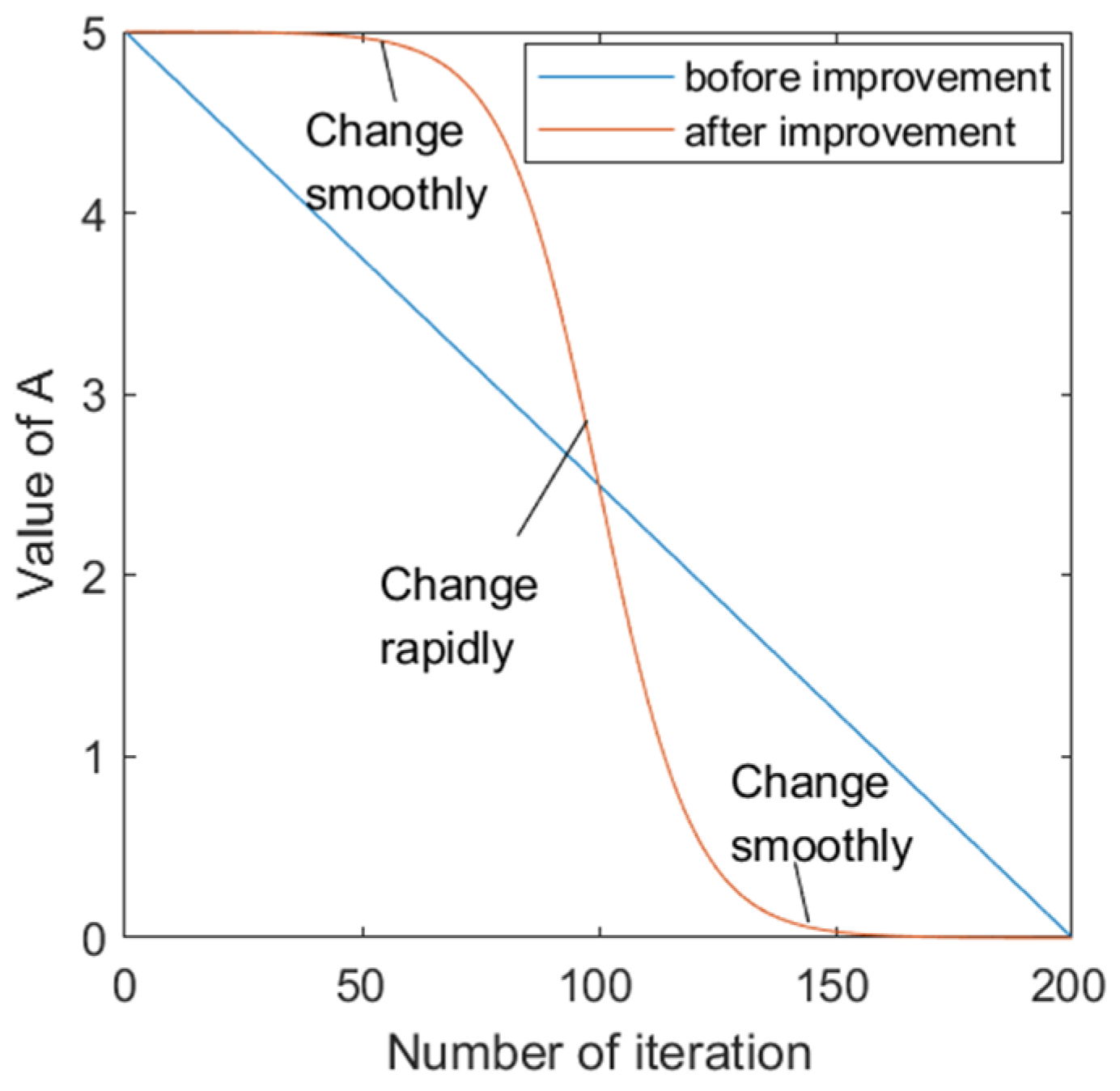
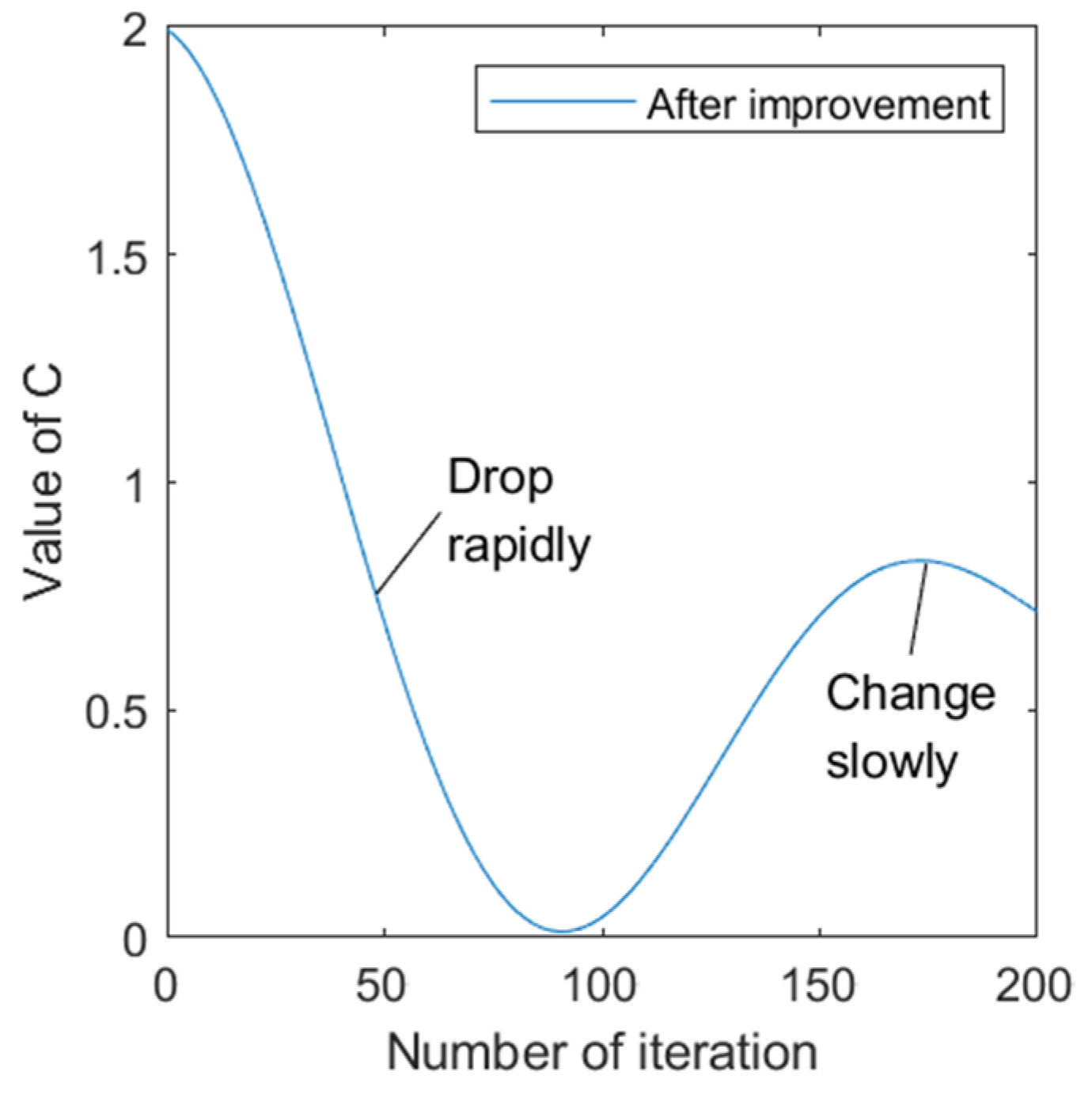
3.2.3. Nonlinear Improvement of Control Factors

In RSO, control factors A and C are used to control the dynamic balance of global search and local search in the iteration process. However, in the traditional calculation, parameter A presents a linearly decreasing relationship with the number of iterations, which lacks the flexibility of dynamic adjustment with the change in the current optimal solution. And parameter C is a random number between [0,2], which has large randomness and blindness. These may cause an imbalance between global search and local search in the iterative process, and reduce the search accuracy of the algorithm. In order to solve the above problems, the nonlinear improvement of parameters A and C is carried out, and the improved calculation formula is as follows.
A = A 0 1 + e 20 t T 10 + β × b p , q
C = C 0 + C 1 1 t T cos 2 π t T + γ t T b p , q
where A 0 and β are the dynamic adjustment factors of parameter A, with values of 5 and 0.2, respectively. b(p,q) is a function that generates random numbers with binomial distribution. C 0 , C 1 , and γ are the adjustment factors of parameter C, and their values are 0.69, 1.3, and 0.03, respectively. The change trend observed in parameters A and C after improvement is shown in Figure 2 and Figure 3.
As can be seen from the figure, the improved factor A takes a larger value when the number of iterations is small, ensuring a wider search range in the early iterations. However, as the change amplitude increases from small to large and the change speed increases from slow to fast, the algorithm converges rapidly. When searching near the optimal solution, the change speed and amplitude will decrease again, ensuring local search with a smaller amplitude near the optimal solution. On the other hand, the improved control factor C initially decreases rapidly from a larger value, enhancing the global search capability of the algorithm. The change trend slows down in the middle iterations, and the value gradually increases when the number of iterations is large, ensuring the local optimization ability of the algorithm. Through the cooperation of the improved parameters A and C, the dynamic balance between the global search and local search of the algorithm is further ensured, enhancing its global search and local optimization capabilities.

3.2.4. Iterative Strategy Based on Differential Evolution

In order to improve population diversity and prevent the iteration process from falling into local optimization prematurely, a gene oscillation mechanism based on differential evolution is introduced. Individuals in the population will be mutated with a certain probability to improve the convergence rate of the algorithm. The oscillation function is as follows:
P r t + 1 = P r t + F · P r 1 t P r 2 t ,   p c > v r P r t B · P , p c v r  
P = A × P r t + C × P b e s t t P r t
where parameter F is the scaling coefficient, which is a random number between 0.2 and 0.8. P r 1 t and P r 2 t are two random individuals in the t-generation population. When the value of the random number pc between [0,1] is greater than 0.9, the algorithm will randomly change the current position to reduce the probability of individuals in the population falling into the local optimal solution. When pc ≤ 0.9, parameter B is used to change the current position towards the direction of the optimal individual in the current population. Parameter B is calculated as follows:
B = 2 b r a n d ( ) b
b = 2 log 2 t T
where t is the current number of iterations of the population, and T represents the maximum number of iterations of the population. Both B and b obtained by the above calculation gradually decrease from slow to fast. Therefore, when pc ≤ 0.9, the search range of individuals in the population is larger when the number of iterations is small, which enables them to approach the optimal solution with a greater probability. With the increase in the number of iterations, the value of B decreases at a faster rate, and the individual search range will also decrease to near the current optimal solution, speeding up the convergence process.

3.2.5. Auxiliary Population
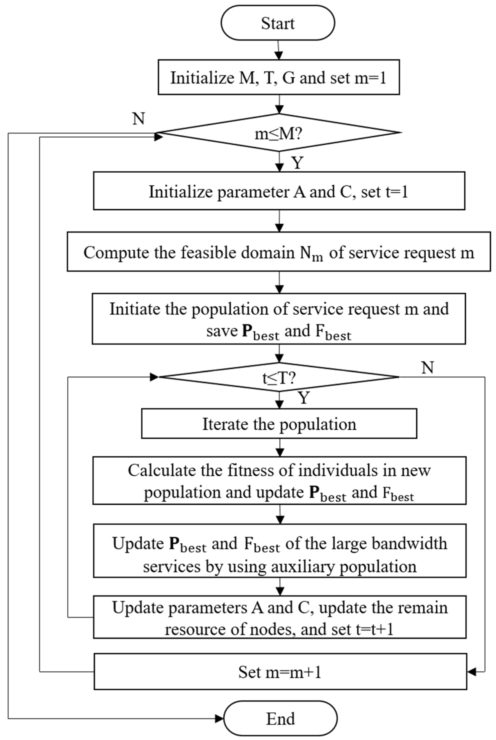
The auxiliary population is introduced to assist the calculation of large-bandwidth services in the iterative process [19]. After obtaining the optimal individual of the population through iteration, for high-bandwidth services, an auxiliary population will be used for further iteration. And the better individual in the auxiliary population will be used to replace the current optimal individual.
The new individual obtained through mutation and cross operation on P r t + 1 is preserved in the auxiliary population, and the mutation and cross processes follow the following formulas:
P r t , k = P r t + F · P r 1 t P r 2 t
v r , t ( i ) = u r , t i , rand 0 , 1 < cr x r , t i ,   otherwise
Individual P r t , k can be obtained by crossing the operation through (26) on individual P r t , k . After the auxiliary population G’ is obtained, the fitness of individuals in the population is calculated. Then, the individual with the highest fitness is selected as the individual P r t + 1 entering the next-generation population. And cr is the probability of mutation.
P r t + 1 = max F P r t , k , k 1,2 , , G

3.3. Algorithm Flow

The specific flow of the MRSO algorithm is as follows Algorithm 1 (Pseudo code):
Algorithm 1 MRSO
Input M, N, Nd, Sr, L, G, G’, T, vr, cr
Output P b e s t , F b e s t
01 for m = 1:M do
02  Initialization parameter A, C, P b e s t and F b e s t ;
03  Calculate N m according to formula (8), (9) and L;
04  for k = 1:G do
05   Randomly generated x k , 1 ;
06   for i = 2:2N do
07    Generate x k , i   according   to   x k , i 1 ,   N m and formula (18);
08     i i + 1;
09   end for
10   Preserve individual P k 0 = ( x k , 1 0 , x k , 2 0 , , x k , 2 N 0 ) ;
11    k k + 1;
12  end for
13  Preserve the optimal individual P b e s t and its fitness F b e s t ;
14  for t = 1:T do
15   for i = 1:G do
16    Calculate individual P i t according to (21) and (22);
17    Calculate fitness value F i t of individual P i ( t ) ;
18    if F i t > F b e s t do
19      P b e s t P i ( t ) ;
20      F b e s t F i t ;
21    end if
22    i i + 1;
23   end for
24   if u m = 1 do
25    for k = 1:G′ do
26   Calculate auxiliary individual P b e s t t , k of P b e s t according to (25) and (26);
27     Calculate fitness value F b e s t t , k of P b e s t t , k ;
28     k k + 1;
29    end for
30    Update P b e s t and F b e s t according to (27);
31   end if
32   Update A and C according to (19) and (20);
33   Update the remaining resources of nodes according to P b e s t ;
34   t t + 1;
35  end for
36 end for
And the following Figure 4 shows the flow chart of the algorithm.
For each service request s r m , it is necessary to conduct two processes: feasible region N m calculation and T iterations of the population. In the process of feasible region calculation, the Dijkstra algorithm is used to compute the nodes that meet the constraints, with a complexity of O( N 2 ). In each iteration of the population, when the optimal resource allocation strategy of the individual is obtained, the time complexity of generating the shortest transmission path is O( N 2 ). And the time complexity of performing iteration with the auxiliary population for large-bandwidth services is O(G′ × 2N), so the time complexity of the T iterations of the population of a service request is O(TG N 2 + 2TG′N). Therefore, the overall time complexity of the algorithm is O(M N 2 + MTG N 2 + 2MTG′N).

4. Simulation Experiment

4.1. Parameter Setting

The simulation environment is set as a square area with a side length of 500 m, containing four types of access networks: 5G, Wi-Fi, ZigBee and mesh networking. The number of nodes in the network is N = 12, and the number of service requests is M = 10. The locations of network nodes and service requests are randomly generated within the area. The communication bandwidth B n n (MHz), caching capacity S n n (GB), caching rate R n n (Mbps) and computing capacity C n n (Gcycle/s) of each network node follow normal distributions, specifically N 1 ~ = ( 2 × 10 3 ,   2 × 10 3 ) , N 2 ~ = ( 50 ,   2 × 10 3 ) , N 3 ~ = ( 100 ,   10 3 ) and N 4 ~ = ( 10 ,   2 × 10 2 ) . The settings for other parameters are shown in Table 1.

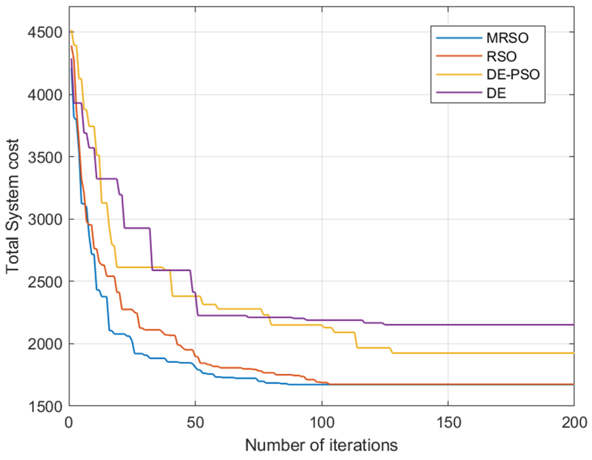
4.2. Simulation Result Analysis

The traditional Rat Swarm Optimization (RSO) algorithm [17], Differential Evolution (DE) algorithm [20] and Particle Swarm Optimization algorithm improved by the same oscillation function (DE-PSO) [21] are selected to compare the iterative effect with the proposed MRSO algorithm. In the experiment, iterations and population sizes that are too high can lead to a waste of computational power and time, while too few iterations and a small population size may result in incomplete searches and difficulties obtaining optimal solutions. Through experimentation, it is found that 200 iterations and a population size of 30 are appropriate values. Therefore, the maximum number of iterations of the above four methods is 200, and the population size is 30. The values of the variation rate (vr) and crossover rate (cr) in the differential evolution algorithm are 0.5 and 0.9, respectively. The number of nodes in the network is N = 12, and the number of service requests is M = 10.
As shown in Figure 5, the comparison of the iterative effects of the four algorithms is presented. Overall, all four algorithms began to converge intensively during the 30th to 100th iterations, converging to 1672, 1675, 1925 and 2152, respectively. Among them, the MRSO algorithm converges faster with a lower total system cost due to the use of multiple strategies to improve the iterative process. However, the traditional RSO algorithm is limited by the iteration strategy and parameter values, resulting in slower convergence compared to MRSO and the risk of falling into local optima. Both DE-PSO and DE exhibit an inferior iterative speed and convergence effects compared to the RSO method. As can be seen from the figure, the MRSO algorithm accelerates the convergence rate, improves the convergence accuracy, and effectively avoids falling into local optima, demonstrating a better iterative performance compared to the other three methods.
In this experiment, two common resource allocation methods, STS-RA [5] and PB-RA, based on the prioritization of service requests [6], were selected for comparison with the MRSO algorithm to verify the effectiveness of the proposed model and method.
As shown in Figure 6 and Figure 7, the system’s total cost and the average processing delay of service requests are presented for the three methods under different numbers of service requests when the number of network nodes N = 12. Overall, the total system costs of all three methods increase with the increase in the number of service requests. When M is set to 10, the total system costs of the three methods are 1671, 1815 and 2160, and the average delays of the service requests are 161 ms, 176 ms and 210 ms, respectively. The MRSO algorithm considers the overall load balancing of the system and can coordinate the allocation of computing, caching, and communication resources among multiple nodes. Therefore, as the number of service requests increases, the increase in the total system overhead is the smallest, and the average processing delay of service requests is also the smallest, with the slowest growth rate as the number of service requests increases. This indicates that the resource allocation strategy calculated by the MRSO algorithm can effectively reduce the total system cost and decrease the average processing delay of service requests.
Figure 8 shows the trend in the total system cost of the three methods, changing with the number of network nodes N when the number of service requests M = 10. On the whole, with the increase in N, the total cost of the system shows a downward trend. When N is set to 12, the total system cost of the three methods is 1675, 1816, and 2157, respectively. With the increase in the number of N, the available resources in the network increase, MRSO always maintains the lowest total system overhead, and the network has a better performance compared with the other two methods when the value of N is small. Also, the total system overhead decreases at a relatively faster rate, indicating the effectiveness of the MRSO algorithm in reducing the total system cost.
Figure 9 shows the changes in system resource utilization as the number of service requests M increases under a high volume of service requests. It can be observed from the figure that the system resource utilization increases with the increase in the number of service requests. However, when the number of service requests exceeds the network’s capacity under the current allocation method, newly generated service requests will be blocked due to timeouts, resulting in no further increase in resource utilization. The resource utilization stops increasing when the number of service requests processed by MRSO reaches 20, indicating that the resource allocation strategy calculated by the MRSO method can support the execution of 20 service requests in the network. Conversely, the other two methods are unable to continue resource allocation after the number of service requests reaches 14 and 18, respectively. This result demonstrates that the MRSO method proposed in this chapter can effectively improve system resource utilization and exhibit robustness in complex network environments.
As shown in Figure 10, the degree of network load balancing under different numbers of service requests is presented when the number of network nodes N = 12. When the number of service requests is small, the difference in the network load balancing among the three methods is not significant. However, as the number of service requests increases, the imbalance in the allocation of network node resources gradually increases, and the differences in the resource allocation strategies obtained by different algorithms become more apparent. With the emergence of more service requests, network node resources are continuously allocated, and the changes in the degree of network load balancing no longer show obvious regularity. However, on the whole, the standard deviation of the resource utilization among nodes using MRSO is the smallest, indicating the most balanced network. This demonstrates the effectiveness of the proposed MRSO in improving the load balancing of the system.

5. Conclusions

In order to address issues regarding the limited resources of individual nodes, inflexible resource allocation and low network resource utilization in local power wireless communication networks, a collaborative allocation model for communicating, caching and computing resources that aims to jointly optimize the system delay and network load balancing is put forward. Furthermore, a multi-strategy-improved Rat Swarm Optimization (MRSO) algorithm is introduced. The simulation results show that compared to the RSO, DE and DE-PSO algorithms, the MRSO algorithm achieves improvements in the solution efficiency of 28.6%, 41.0% and 42.3%, respectively. In addition, compared to the STS-RA and PB-RA resource allocation methods, the total system delay is reduced by 6.7% and 22.4%, respectively, and the utilization rate of network resources is also significantly improved.

Author Contributions

Methodology, J.T. and S.S.; Software, J.T.; Validation, S.S.; Formal analysis, Y.W.; Investigation, J.T. and S.W.; Resources, Y.W. and S.W.; Writing—original draft, J.T.; Supervision, S.G.; Project administration, S.S.; Funding acquisition, S.G. All authors have read and agreed to the published version of the manuscript.

Funding

This work was funded by Ningxia Natural Science Foundation (No. 2023AAC03859).

Institutional Review Board Statement

Not applicable.

Informed Consent Statement

Not applicable.

Data Availability Statement

The data presented in this study are available on request from the corresponding author.

Conflicts of Interest

Authors Ye Wang and Shuang Wu were employed by the company State Grid Ningxia Electric Power Co., Ltd. The remaining authors declare that the research was conducted in the absence of any commercial or financial relationships that could be construed as a potential conflict of interest.

References

  1. Yang, Q.; Zhu, C.; Liu, S.; Yian, J. Key Technologies of Heterogeneous Network in Power Communication Systems. Power Energy 2021, 42, 46–50. [Google Scholar]
  2. Culler, D.E. The Once and Future Internet of Everything. GetMobile Mob. Comput. Commun. 2017, 20, 5–11. [Google Scholar] [CrossRef]
  3. Amini, M.R.; Baidas, M.W. Performance Analysis of Grant-Free Random-Access NOMA in URLL IoT Networks. IEEE Access 2021, 9, 105974–105988. [Google Scholar] [CrossRef]
  4. Liao, Y.; Yu, Q.; Han, Y.; Leeson, M.S. Relay-Enabled Task Offloading Management for Wireless Body Area Networks. Appl. Sci. 2018, 8, 1409. [Google Scholar] [CrossRef]
  5. Han, Q.; Fang, X. Resource Allocation Schemes of Edge Computing in Wi-Fi Network Supporting Multi-AP Coordination. Comput. Syst. Appl. 2022, 31, 309–319. (In Chinese) [Google Scholar]
  6. Ji, W.; Tang, W.; Ding, S.; Wang, S.; Jiang, Q.; Zhou, A.; Sun, Q. Resource Cooperative Allocation Method and Device in Mobile Edge Computing Network. CN115022928A, 6 September 2022. [Google Scholar]
  7. Ndikumana, A.; Tran, N.H.; Ho, T.M.; Han, Z.; Saad, W.; Niyato, D.; Hong, C.S. Communication, Computation, Caching, and Control in Big Data Multi-Access Edge Computing. IEEE Trans. Mob. Comput. 2019, 19, 1359–1374. [Google Scholar] [CrossRef]
  8. Fan, Q.; Lin, J.; Feng, G.; Gao, Z.; Wang, H.; Li, Y. Joint Service Caching and Computation Offloading to Maximize System Profits in Mobile Edge-Cloud Computing. In Proceedings of the 2020 16th International Conference on Mobility, Sensing and Networking (MSN), Tokyo, Japan, 17–19 December 2020; pp. 244–251. [Google Scholar]
  9. Wang, C.; Liang, C.; Yu, F.R.; Chen, Q.; Tang, L. Computation Offloading and Resource Allocation in Wireless Cellular Networks With Mobile Edge Computing. IEEE Trans. Wirel. Commun. 2017, 16, 4924–4938. [Google Scholar] [CrossRef]
  10. Zhang, J.; Hu, X.; Ning, Z.; Ngai, E.-C.H.; Zhou, L.; Wei, J.; Chen, J.; Hu, B.; Leung, V.C. Joint Resource Allocation for Latency-Sensitive Services over Mobile Edge Computing Networks with Caching. IEEE Internet Things J. 2019, 6, 4283–4294. [Google Scholar] [CrossRef]
  11. Song, Y.; Li, X.; Ji, H.; Zhang, H. Joint Computing, Caching and Communication Resource Allocation in the Satellite-Terrestrial Integrated Network with UE Cooperation. In Proceedings of the 2022 IEEE/CIC International Conference on Communications in China (ICCC), Foshan, China, 11–13 August 2022; pp. 604–609. [Google Scholar]
  12. Xia, W.; Shen, L. Joint resource allocation using evolutionary algorithms in heterogeneous mobile cloud computing networks. China Commun. 2018, 15, 189–204. [Google Scholar] [CrossRef]
  13. Yang, Z.; Xie, J.; Gao, J.; Chen, Z.; Jia, Y. Joint Optimization of Wireless Resource Allocation and Task Partition for Mobile Edge Computing. In Proceedings of the 2020 IEEE/CIC International Conference on Communications in China (ICCC), Chongqing, China, 9–11 August 2020; pp. 1303–1307. [Google Scholar]
  14. Dab, B.; Aitsaadi, N.; Langar, R. Joint Optimization of Offloading and Resource Allocation Scheme for Mobile Edge Computing. In Proceedings of the 2019 IEEE Wireless Communications and Networking Conference (WCNC), Marrakesh, Morocco, 15–18 April 2019; pp. 1–7. [Google Scholar]
  15. You, C.; Huang, K.; Chae, H.; Kim, B.-H. Energy-Efficient Resource Allocation for Mobile-Edge Computation Offloading. IEEE Trans. Wirel. Commun. 2017, 16, 1397–1411. [Google Scholar] [CrossRef]
  16. Zhang, Y.; Li, Y.; Huang, H.; Zhuang, H. Joint optimization algorithm for task offloading and resource allocation in heterogeneous networks. J. Beijing Univ. Posts Telecommun. 2022, 45, 91–97. [Google Scholar]
  17. Dhiman, G.; Garg, M.; Nagar, A.; Kumar, V. A novel algorithm for global optimization: Rat Swarm Optimizer. J. Ambient Intell. Humaniz. Comput. 2021, 12, 8457–8482. [Google Scholar] [CrossRef]
  18. Xie, R.; Hai, B. The Path Planning of Robot Based on Multi-strategy Rat Swarm Optimizer. Mod. Mach. Tool Autom. Manuf. Tech. 2022, 10, 50–54. [Google Scholar]
  19. Guo, P. Research on Improvement of Differential Evolution Algorithm; Tianjin University: Tianjin, China, 2012. [Google Scholar]
  20. Zhang, J.; Zhao, H.; Li, T.; Zhao, X.; Wang, Y. Joint Task Offloading and Resource Allocation Method Based on Multi-Objective Optimization. J. Nanjing Norm. Univ. (Nat. Sci. Ed.) 2024, 47, 121–132. [Google Scholar]
  21. Zhang, L.; Wang, M. Joint Optimization Algorithm of Edge Computing Offloading and Computing Resource Allocation. J. Command Control 2023, 9, 323–334. [Google Scholar]
Figure 1. System scene diagram.
Information 15 00309 g001
Figure 2. The change trend of parameter A before and after improvement.
Information 15 00309 g002
Figure 3. The change trend of improved parameter C.
Information 15 00309 g003
Figure 4. Algorithm flow chart.
Information 15 00309 g004
Figure 5. Comparison of the solving efficiency of different algorithms.
Information 15 00309 g005
Figure 6. Influence of the number of service requests on total system cost.
Information 15 00309 g006
Figure 7. Influence of the number of service requests on average delay.
Information 15 00309 g007
Figure 8. Influence of the number of network nodes on total system cost.
Information 15 00309 g008
Figure 9. Influence of the number of service requests on the utilization rate of system resources.
Information 15 00309 g009
Figure 10. Influence of the number of service requests on the degree of system load balance.
Information 15 00309 g010
Table 1. Simulation parameters.
Parameter DescriptionSymbolValue/Unit
Bandwidth required by service request m B m 1~800 Mbps
Computing resource required by service request m C m 0.2~4 Gcycles
Caching resource required by service request m S m 1~10 GB
The amount of data transferred by the service request m D m 0.1~4000 Mbit
Maximum tolerated latency of service request m τ 10~300 ms
Weight coefficient λ 320
Noise power σ 2 2 × 10 13
Transmission power of node n P n 0.1~1 W
Proportional coefficientμ0.1
Disclaimer/Publisher’s Note: The statements, opinions and data contained in all publications are solely those of the individual author(s) and contributor(s) and not of MDPI and/or the editor(s). MDPI and/or the editor(s) disclaim responsibility for any injury to people or property resulting from any ideas, methods, instructions or products referred to in the content.

