Article

Analyzing Biomedical Datasets with Symbolic Tree Adaptive Resonance Theory

1
Department of Electrical and Computer Engineering, Missouri University of Science and Technology, Rolla, MO 65409, USA
2
Department of Neurology and Rehabilitation, University of Illinois at Chicago, Chicago, IL 60607, USA
3
Department of Science and Industry Systems, University of Southeastern Norway, 3616 Kongsberg, Norway
4
Engineering Program, Missouri State University, Springfield, MO 65897, USA
5
Honeywell Federal Manufacturing & Technologies, Kansas City, MO 64147, USA
*
Author to whom correspondence should be addressed.
Information 2024, 15(3), 125; https://doi.org/10.3390/info15030125
Submission received: 29 January 2024 / Revised: 9 February 2024 / Accepted: 10 February 2024 / Published: 23 February 2024

Abstract

:
Biomedical datasets distill many mechanisms of human diseases, linking diseases to genes and phenotypes (signs and symptoms of disease), genetic mutations to altered protein structures, and altered proteins to changes in molecular functions and biological processes. It is desirable to gain new insights from these data, especially with regard to the uncovering of hierarchical structures relating disease variants. However, analysis to this end has proven difficult due to the complexity of the connections between multi-categorical symbolic data. This article proposes symbolic tree adaptive resonance theory (START), with additional supervised, dual-vigilance (DV-START), and distributed dual-vigilance (DDV-START) formulations, for the clustering of multi-categorical symbolic data from biomedical datasets by demonstrating its utility in clustering variants of Charcot–Marie–Tooth disease using genomic, phenotypic, and proteomic data.

1. Introduction

Precision medicine depends upon a detailed unraveling of the relationships between diseases, phenotypes, genes, and the underlying proteins and biological pathways [1,2,3,4,5,6,7]. The ready availability of protein, disease, gene, phenotype, and biological pathway ontologies makes it possible to construct purpose-specific datasets for studying human disease. These can take the form of symbolic relationships that can be organized into formal ontologies that are instantiated as knowledge graphs defining the permissible relationships between classes and the instances within them [8].
However, many elements in these disease–gene–protein datasets are formatted as categorical rather than numerical variables, bringing a unique challenge to machine learning algorithms. Although tools exist to analyze and visualize categorical data [9], the tools for clustering these datasets depend heavily on recasting categories into real-valued spaces, which is largely unavoidable due to the definition of the problem statement; all modalities of machine learning assume distance metrics or similarity measures of their feature spaces, whereas categorical data contain symbols that do not belong to ordered sets, and thus, do not inhabit metric spaces. An important design choice then when working with mixed or fully categorical data is how to recast categorical features into spaces with similarity measures [10]. This recasting, whether by one-hot encoding, ordinal encoding, or another encoding scheme, can bring its own deleterious consequences; one-hot encoding of categories can generate large sparse feature vectors due to many different categories, while ordinal encoding can introduce measures of proximity between categories that do not intrinsically exist. Meta-analyses of symbolic datasets may yield similarity meta-metrics that are useful for clustering [11,12], but these meta-metrics require domain knowledge of the categories in the dataset, limiting both their transferability to other datasets and applicability to streaming learning. While statistical machine learning algorithms can compensate for some of these input feature space shortcomings through sophisticated machinery that relies on a large dataset size and a high degree of feature cardinality, these methods naturally suffer in regimes with small categorical datasets. Furthermore, these encoding schemes and the machine learning algorithms do not gracefully extend to instances of hierarchical or nested attributes such as occur with the variably sized association of diseases with phenotypes, genes, and proteins.
Adaptive resonance theory (ART) algorithms principally belong to the class of incremental neurogenesis clustering/unsupervised [13] algorithms, with many additional variants for use in supervised learning [14,15], reinforcement learning [16,17], and even self-supervised and multimodal applications [18]. The design of these algorithms allows them to update existing categories or create new ones from the data alone in a stable, incremental, and lifelong manner. With the notable exception of the binary-valued ART1 algorithm, most of these algorithms work upon real-valued preprocessed feature datasets via the use of fuzzy feature membership [19,20,21,22,23]. In contrast, the Gram-ART algorithm was designed for the meta-optimization of genetic algorithms, and thus, is designed to work with variable-length symbolic datasets [24], but it too has its shortcomings when tackling the large numbers of terminal symbols encountered in medical disease datasets.
With these myriad design challenges in mind, this article describes the design of a new ART algorithm named symbolic tree adaptive resonance theory (START) for the clustering of variable-length symbolic statements. This formulation of START also includes both dual-vigilance (DV-START) and distributed dual-vigilance (DDV-START) variants [25,26] along with their supervised modifications. This article also outlines methods for casting categorical disease–gene biomedical datasets into symbolic datasets for both unsupervised clustering and supervised training where labels are available.
The changes in START compared to the Gram-ART algorithm summarize the novel contributions of this article in addition to the use of this algorithm for the study of biomedical disease-variant data. START extends Gram-ART as a novel approach to analyzing biomedical disease-variant data in the following ways:
  • Both a match and activation function for the Gram-ART match rule.
  • Optimizations to the prototype-encoding scheme to mitigate memory complexity in grammars with large sets of terminal symbols.
  • A mechanism to grow prototype tree structures when novel production rule sets are encountered.
  • Both dual-vigilance and distributed dual-vigilance START variants [25,26].
  • A supervised modification for each unsupervised START variant.
This article is organized into the following sections: Section 2 provides a background of the literature pertinent to the formulation of START, while Section 3 describes the derivation and structure of START and its dual-vigilance and supervised variants. Section 4 outlines the datasets and experimental methodology utilized in the evaluation of START, including benchmark machine learning datasets and the target biomedical disease-variant datasets of the article, and Section 5 contains the results of these experiments. Section 6 discusses the experimental results and their biological plausibility, with Section 7 providing final conclusions on both START and the biomedical dataset analysis of the previous sections.

2. Background

2.1. Adaptive Resonance Theory

Adaptive resonance theory (ART) is a neurocognitive theory of how biological neural networks for self-stable representations learn without catastrophic forgetting, online and without supervision, through feedback and competitive dynamics [27,28,29,30,31,32,33,34,35]. Since its inception, a variety of machine learning models have been implemented using the theory as a basis [19,36,37,38]. Though these algorithms in large part belong to the class of incremental neurogenesis clustering/unsupervised algorithms, they have been adapted for applications in supervised, reinforcement, and even multimodal learning [19,39], tackling clustering issues from sample granularity [25,26] to distributed representations [40,41,42], pattern sequences [43], context recognition [44,45], and uncertainties [46,47,48]. Some algorithms based upon ART have even been combined with incremental cluster validity indices (ICVIs), metrics of clustering performance in the absence of supervised labels, to enable a variety of incremental, online, and multimodal clustering and biclustering applications [49,50,51,52,53,54]. ART algorithms are additionally well suited for lifelong learning (L2) applications because they are derived from theories on how biological neural networks address the stability–plasticity dilemma to mitigate catastrophic forgetting [55,56,57].
Nearly all ART formulations trade the explicit coarseness parameters of other clustering algorithms for a vigilance parameter ( ρ ( 0 , 1 ) ), which behaves as a threshold of agreement between a sample and expectations to determine whether to update existing knowledge or to create new categories altogether, a process known as the ART match rule [41]. Furthermore, nearly all ART formulations are intrinsically prototype-based machine learning algorithms, meaning that categories are defined by representative prototypes in the sample feature space. This has two important consequences: ART algorithms theoretically have unlimited memory because new prototypes may always be instantiated, but they generally have no representational capacity in the sense of manifold learning, relying instead on the assumption that the feature space being used for clustering is sufficiently well separated. Samples in this feature space are provided in a feature representation layer F 1 , which is compared with a category representation layer F 2 containing these prototypes through ART competitive dynamics that include a check against this vigilance parameter.

2.2. Gram-ART

Gram-ART is a clustering algorithm, based on ART learning dynamics, that defines its prototypes and input features as trees of parsed statements adhering to a formal grammar [24]. Originally designed to tackle the problem of comparing similarity between symbolic expressions for the meta-optimization of genetic algorithms, it is capable of accepting statements of an arbitrary length according to a user-defined context-free grammar (CFG) expressed in the Backus–Naur form (BNF). In the original formulation, Gram-ART samples are statements adhering to a CFG that are parsed into rooted syntax trees. These parsed samples are then compared according to ART learning rules to Gram-ART prototypes that are themselves rooted trees containing distributions of terminal symbols that are encountered at each node during learning. Gram-ART answers the questions of how to formulate prototype trees of varied shape, compute similarities of sample statements to prototypes of differing shapes, and update the terminal symbol distributions at each node during learning.
Gram-ART is the first ART algorithm capable of clustering inputs samples of arbitrary length, but it also inherits some problems from working with symbolic data. Terminal symbols under a grammar have no fuzzy membership or relation without an additional embedding scheme. Gram-ART tackles this by updating distributions of terminal symbols at each position along the rooted prototype trees during learning. However, this technique quickly grows in space and subsequent time complexity in grammars with sets of terminal symbols larger than the algebraic expressions that they were originally designed for.

3. Method

3.1. START: Symbolic Tree Adaptive Resonance Theory

This paper introduces a new formulation of the Gram-ART algorithm called START for the clustering of symbolic datasets. START is a prototype-based unsupervised clustering algorithm that when presented with a new sample utilizes ART dynamics to determine whether to update an existing template or to instantiate a new one. START targets symbolic expressions adhering to a context-free grammar CFG ( T , N , P , S ) with a complete set of terminal symbols T , non-terminal symbols N , production rules P , and a statement entry point S . The prototypes of START are rooted trees containing learned distributions of the encountered terminal symbols at each node representing a non-terminal position, and symbolic statements are parsed into rooted constituency parse trees that are subsequently processed against these prototypes using ART learning dynamics. With such a formulation, the method is naturally extended to the clustering of purely categorical datasets of variable length sequences, such as in the myriad categorical fields of disease–gene–protein data.

3.1.1. Motivation

The realm of clustering, and indeed machine learning as a whole, requires a serious consideration and study of the various forms that data may take [10]. Datasets are often modeled as samples of the state space defined by some measuring device. Many samples of data are naturally real-valued, such as the readings from imaging sensors for the purposes of computer vision, while others are categorical in nature, such as descriptor labels of the color of an object (e.g., red, blue, yellow). Datasets may have one or more feature dimensions, and they may even be multimodal, containing a combination of real-valued and categorical data in each sample. A notion of the proximity of features is critical to machine learning algorithms that utilize similarity measures to model and interpret samples; metric spaces are defined as sets that can have such a similarity measure defining the distance between points in the set, and indeed even categorical features may sometimes have distance metrics if they have an ordering (e.g., low, medium, high), though they often only have a strict equivalence relation for comparing categories (e.g., red = red, red ≠ blue). The presence of a distance metric is especially important in unsupervised learning scenarios such as clustering where an algorithm has nothing available to model a dataset aside from the features themselves. As a consequence, the clustering of data with unordered categorical features is difficult, and many clustering algorithms are designed with the assumption that at least some ordered features exist in the data [10].
Nevertheless, purely categorical datasets such as those containing only label descriptors do exist, and it is desirable to cluster them to extract meaning and structure. It is even more challenging when such datasets contain a varying number of features for each sample; algorithms that tackle real-valued datasets of variable length such as time-series data utilize techniques like convolutions and pooling to turn a varying number of features at runtime into a fixed model size, but these techniques are ill-defined for purely categorical data, especially when individual symbols are sparsely populated throughout the dataset.
Purely categorical datasets of variable feature dimensions arise commonly in human-annotated datasets, such as those generated from medical research. Human-prescribed categories of diseases, their variants, and other ontological features can contain missing entries when data are missing or inapplicable, and categories can even be nested; for example, the presence or absence of the symptom of pain may be further qualified by pain in specific regions of the body or of varying intensity according to some pain scale.
One realm that specifically deals with categorical data of variable length is the study of languages [58,59]. Syntactically, sentences in a language are interpreted as statements that adhere to a formal grammar that determines the rules of what is or is not a valid statement in a given language. The study of language also applies in the design of lexers and parsers, which are used in computer science for the design of programming languages to structure valid symbolic statements of arbitrary length written by a programmer for compilation or interpretation. Parsers are especially important as a mechanism of applying the rules of a grammar to interpret strings of symbolic statements as syntax trees defining their structure. These grammar rules, however, do not define a notion of how similar or dissimilar two statements are, so a clustering algorithm working in this space must introduce a mechanism for comparing statement similarity.
Given that START shares the objective of Gram-ART to cluster variable-length symbolic expressions, the key design challenges of START’s design are in how to formulate metrics of similarity between these symbolic expressions. In such a formulation, statements are collections of symbols sampled from unordered sets; individual symbols share no fuzzy membership, so similarity between symbols is dictated by strict equivalence in a set theoretic sense. Furthermore, though statements of equal length introduce a step-wise fuzziness when symbols in the same relative positions are identical, many datasets do not satisfy the assumption of equivalent non-terminal structure across all statements. In the pursuit of creating a clustering algorithm for variable-length symbolic datasets, START utilizes a prototype method as a proxy for direct comparison between statements, using ART-based competitive learning dynamics for determining when to update templates and when to instantiate new ones. As with all ART algorithms, START therefore inherits both the theoretically unlimited learning capacity of neurogenesis algorithms and the problems of category proliferation that they bring; though new prototypes can be instantiated for an arbitrary number of categories, this growing knowledge base incurs its own search time complexity [19,60].

3.1.2. START Algorithm

START shares the nomenclature of Gram-ART and other ART algorithms from its structure to its learning dynamics, so existing terminology is preferred where available. START also follows the procedure of most ART unsupervised clustering algorithms, with additional considerations for handling symbolic data. As in Gram-ART, START handles this symbolic data by working in the space of the syntactic trees representing the symbolic data as statements under a formal grammar. The shared notation of all START variants is listed in Table 1.
A START module is initialized to contain the CFG ( T , N , P , S ) rules of the target symbolic dataset statements. This grammar can be inferred from an existing dataset of statements if all relevant symbols and production rules are represented in the dataset. Statements from the dataset are parsed according to the production rules of the grammar into rooted constituency parse trees, the basic unit of which is known in Gram-ART and START as a TreeNode. Each parsed statement tree is presented incrementally to the START module, and each sample either mutates an existing prototype or is used to instantiate an entirely new prototype [19]. Prototypes in START are themselves rooted trees with a structure modified from the statement trees, the basic unit of which is known in Gram-ART as a ProtoNode. The stateful information of START TreeNodes and ProtoNodes can be seen in Table 2 and Table 3, respectively.
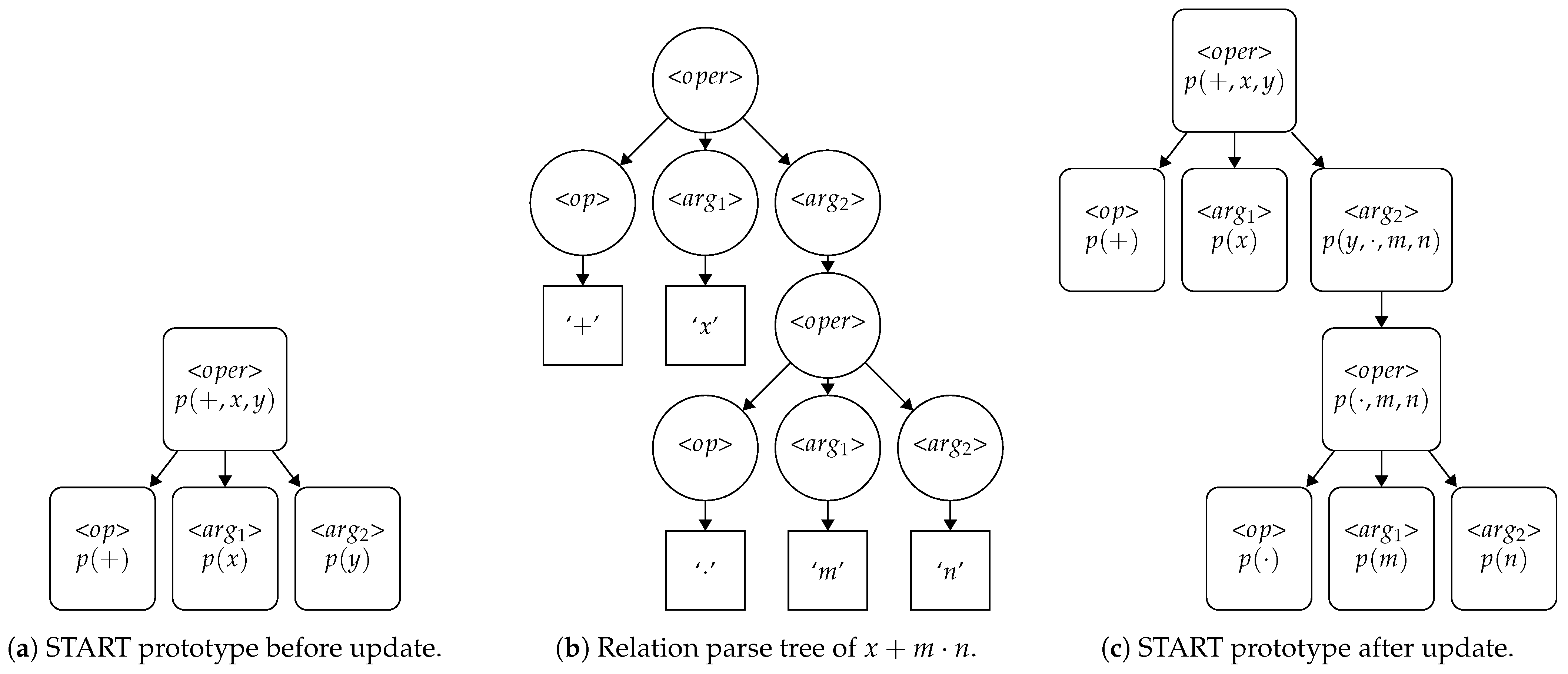
Here, START and Gram-ART differ on an important point in formulation: Gram-ART treats ProtoNodes and TreeNodes as modified dependency relation syntax trees where each node represents a terminal symbol, the children of which are the dependents of that symbol. This formulation is most apparent in the case of operators, such as in the algebraic statement x + y , where the operator terminal + would have branch dependents x and y. In START, however, ProtoNodes and TreeNodes are defined as relation parse trees with non-terminal symbols representing non-terminal positions and terminal symbols at the leaves of the rooted tree. The same algebraic statement x + y is then treated in START as a relation parse tree with non-terminal symbols for the operation and its three branches represent the operator and its two arguments, with leaf nodes realizing the terminal symbols at these non-terminal positions (Figure 1).
In START, sample symbolic statements are preprocessed into parse trees via a syntactic parser such as an Earley parser according to the production rules P of the grammar written most generally in an extended Backus–Naur form (EBNF) [61,62]. These syntax trees can be interpreted as concrete constituency relation parse trees belonging to constituency grammars, also known as phrase structure grammars, where branches of a parse tree are all non-terminal symbols in the grammar, including the statement entry point, and leaf nodes are terminal symbols [58,59]. These parse trees are then converted to statement trees via an inclusion of metadata at each node indicating the symbol to be terminal or non-terminal. Prototypes in START are rooted trees containing probability mass functions (PMFs) of terminal symbols encountered at and below the position of each ProtoNode on the tree. In contrast with Gram-ART, these START prototypes do not contain terminal symbol leaves; instead, the nodes of the prototypes represent the non-terminal positions of the grammar production rules applied to the node’s position on the tree, which reduces the effective size of each prototype tree while still encoding the occurrence of terminal symbols at and below those positions via their PMFs.
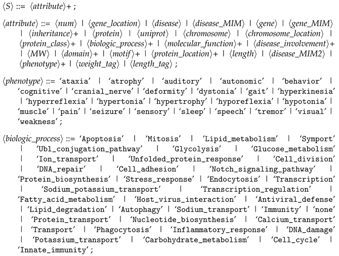
Listing 1. Formal grammar for parsing Charcot–Marie–Tooth disease–protein flat-file data. EBNF syntax is used for production rules with the exception of the regular expression symbol ‘+‘, which is used to denote one or more occurrences of the preceding symbol. Statements are composed of a series of one or more categorical attributes, all of which are listed in the non-terminal symbol <attribute>. When an attribute is missing or otherwise unknown for a CMT variant, then it is not included in the parsed syntax tree and handled accordingly by START. The production rules for two notable multi-category attributes, < p h e n o t y p e > and < b i o l o g i c _ p r o c e s s >, are listed to demonstrate how statements formulated from CMT disease-variant entries illustrate how a gene can be associated with multiple phenotypes and biologic processes. Other multi-category attributes are not listed for brevity.
Information 15 00125 i004

3.1.3. Derivation of the START Match Rule

A fundamental characteristic of ART algorithms is the use of a match rule, whereby a process of bottom-up activations drive the evaluation of how much the input sample matches existing top-down categories [41]. Because of the origins of these algorithms lies in the analysis of the competitive dynamics of biological neural networks, these activation and match functions are frequently analogized with bottom-up prediction and top-down expectation, respectively.
Gram-ART utilizes an activation function, while START introduces separate activation and match functions. The distinction between the two lies in the normalization scheme of the activation and match functions; for example, in ART1 the match function (Equation (2)) is the activation function (Equation (1)) normalized by the size of the input [19].
T j = x w j 1
M j = y F 1 1 x 1 = x w j 1 x 1
FuzzyART replaces the binary intersection with the fuzzy intersection in both equations and normalizes the activation by the magnitude of the weight vector [19]. When evaluated at a single node, an input terminal symbol can be interpreted as a one-hot binary vector encoding at the terminal symbol position, so the magnitude of the membership of sample x in weight w j is indeed the fuzzy intersection x w j 1 . This is computed in START for the terminal distribution of each ProtoNode climbing up from the aligned leaf representing the terminal symbol. In statements with many branches arising from non-trivial production rules, this means the evaluation of the activation at each ProtoNode for potentially multiple terminal descendants.
The activation is then normalized by the size of the input pattern, which can be realized in multiple manners requiring a design decision; with the rooted tree definition of parsed input statements, the size of the input pattern could be interpreted as the number of nodes in the parsed statement, the number of terminal symbols in the unparsed statement, or a more complex function of the number of terminals that could be realized beneath the non-terminal position of the node in question according to the production rules of the grammar of the sample. For simplicity, the remainder of this study utilizes the length of the unparsed statement itself as a normalizing factor, having the effect of discounting the disproportional contributions to the match value of increasingly longer statements. In grammars where statements are of equal length, such as in the processing of tables with single-category data, each decision trivially scales the required vigilance values to satisfy the vigilance criterion.
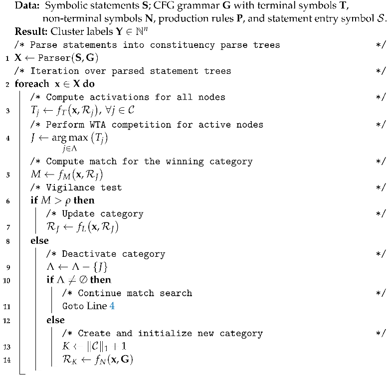
The remainder of the match rule follows the activation, competition, match, and vigilance test of unsupervised ART algorithms, as can be seen in Algorithm 1, with the exception of the dual-vigilance variants of START, which can be seen in Section 3.1.5 and Algorithm 2.

3.1.4. Derivation of the Weight Update

When a prototype is selected for learning according to the START match rule, the input TreeNode and selected ProtoNode are root-aligned and compared, similar to in the activation and match processes. The terminal symbols contributing to the activation and match functions of the winning prototype are used for updating the PMF at each non-terminal symbol position at each ProtoNode up the prototype tree. The instance count of the observed terminal symbol is incremented, and the PMF update is weighted by the instance count of each terminal of the distribution to renormalize. In Equation (3), the weight value w of the PMF indexed at terminal T in node i is updated with instance count N and a Kronecker delta δ T that is satisfied if the terminal symbol x being evaluated is equivalent to the PMF index T (Equation (4)).
w i T = w i T N + δ T x N + 1
δ T x = 1 if T = x 0 otherwise
Algorithm 1: START algorithm. A set of symbolic statements under a formal context-free grammar are parsed into their syntax trees. Prototypes are defined as learning dynamics otherwise follow the activation, competition, match, update, and initialization rules of unsupervised ART algorithms [19]. ART dynamics notation here largely follow the elementary ART algorithm outlined in [19]. Inference during classification follows the same match rule dynamics without the instantiation of new categories; in the case of complete mismatch, either an “unknown” label or the best matching unit (the category that maximizes the match criterion) may be returned. Please see Table 1 for full notation
Information 15 00125 i001
If no prototype satisfies the vigilance criterion, a new one is instantiated. START prototypes do not encode all combinations of non-terminal production evaluations during instantiation, as this would quickly combinatorially explode towards the Catalan number of the non-terminal production rules, and it could be infinite in some recursive grammars. Instead, prototypes are instantiated as structural clones of the input TreeNode without the inclusion of the terminal symbols at their leaves. This design decision is made to mitigate the time and memory complexity of the ProtoNode evaluation given that the non-terminal node preceding a terminal leaf already encodes all of the instances that the terminal symbol encounters. The new structural clone prototype is then trained upon the input sample, updating the PMFs of each ProtoNode for the first time. In the case that an existing winning prototype does not contain the input TreeNode as a structural subset (i.e., it is missing a non-terminal production rule path describing the parsed TreeNode), these new non-terminal paths are instantiated on the winning prototype and updated as usual.
Algorithm 2: Dual-Vigilance START algorithm. This algorithm combines Algorithm 1 with the dual-vigilance procedure of DVFA [25]. The vigilance test is split into a cascade of two vigilance checks for the current match candidate node. Passing the upper vigilance check updates the current category node, while passing only the lower vigilance check creates a new category node belonging to the same cluster label. Failing to pass both vigilance checks results in the instantiation of a new category node belonging to an incrementally new cluster label. Please see Table 1 for full notation
Information 15 00125 i002

3.1.5. Dual-Vigilance and Distributed Dual-Vigilance START

The FuzzyART algorithm provides a foundation for how to adapt ART learning rules to real-valued datasets [19]. Like most ART modules, FuzzyART utilizes the ART match rule evaluated at a single threshold value that is either the vigilance hyperparameter ρ or a function thereof. Dual-vigilance FuzzyART (DVFA) utilizes instead two vigilance parameters for the match rule evaluation, a lower bound ρ l b and upper bound ρ u b , which separates prototypes in a many-to-one mapping from categories to clusters and introduces the ability to compensate for differing granularity both within and between clusters [25]. Distributed dual-vigilance FuzzyART (DDVFA) advances this idea by representing entire clusters with FuzzyART modules governed by a global FuzzyART module, compensating for even varying granularity within different clusters and enabling the ability to learn arbitrary cluster shapes [26]. Each node in the global F2 layer competes for assignment of a provided sample through modified activation and match linkage methods, defining the relevant proximity measures of the sample to an entire F2 FuzzyART module node.
The principles of dual-vigilance and distributed dual-vigilance are extended here for START. In the dual-vigilance formulation (DV-START), the same cascading technique as in DVFA is used for determining category–cluster assignments through upper- and lower-bound vigilance hyperparameters during the ART match evaluation:
  • M J > ρ u b : if the current match candidate satisfies the upper vigilance threshold, then the winning category is updated according to the START weight update rules.
  • ρ u b > M J > ρ l b : if the current match candidate only satisfies the lower vigilance threshold but not the upper, then a new category prototype is instantiated that belongs to the same cluster as the winning node.
  • ρ l b > M J : if the current match candidate does not satisfy even the lower-bound vigilance threshold, then the normal mismatch procedure is followed, where a new category is instantiated belonging to an entirely new cluster.
In the distributed dual-vigilance formulation (DDV-START), additional modifications are made to accommodate the rooted tree structures of the prototypes. DDVFA utilizes a global FuzzyART module that represents nodes themselves as FuzzyART modules [26]. The basic units of DDV-START are the rooted ProtoNode trees, but global module dynamics are not restricted to their use; because the global module of DDV-START is largely agnostic to the formulation of the input samples, the global module may be approximated as a FuzzyART module coordinating the learning of its START F2 nodes. With the exception of the centroid linkage method, which in DDVFA is defined as a function of local FuzzyART weights, all other linkage methods from DDVFA can be utilized in DDV-START; by independently defining the activation and match values for each ProtoNode within an F2 START module, the global values can be compared using the hierarchical agglomerative clustering (HAC) methods of DDVFA, as can be seen in Table 4.

3.1.6. Supervised Variants

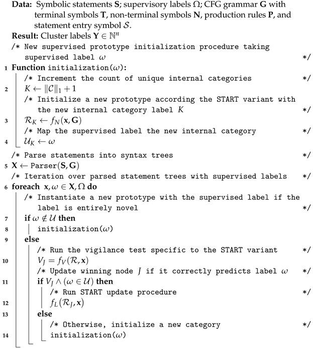
Most ART algorithms are designed as unsupervised clustering algorithms with variants and compositions of the elementary ART module motif providing supervised and reinforcement learning variants [19]. ARTMAP is a formulation of ART, comprised of two elementary ART modules and an inter-ART map field, that enables multidimensional mapping between two feature fields [63]. A simplified version of FuzzyARTMAP, where the second module A R T B is replaced with vectors representing class labels, provides a basic procedure for adapting unsupervised ART modules to simple supervised ARTMAP variants [64]. Though START is designed as an unsupervised clustering algorithm, it utilizes these supervised modifications for evaluation on the supervised machine learning benchmark datasets in Section 4.2 and in the Supplementary Materials of this paper. Algorithm 3 outlines this procedure of mapping the internal category representation labels to supervised labels for any START variant.
Because these supervised variants are derived from a procedure to modify an ART module to a simplified ARTMAP variant, their naming follows the same notation (e.g., START to Simplified STARTMAP).

3.1.7. Summary of START Variants

The previous sections have outlined three unsupervised algorithms for the clustering of categorical data of varying feature dimensionality: START, its dual-vigilance variant DV-START, and its distributed dual-vigilance variant DDV-START. The core START algorithm is outlined for clustering this categorical data using the incremental learning and update rules of ART algorithms with a single vigilance value; if a category match is found, that prototype is updated according to the ART match rule, and if there is instead a complete mismatch, a new category is instantiated. The dual-vigilance (DV-START) and distributed dual-vigilance (DDV-START) variants of this core algorithm follow as extensions of the algorithm through modifications of the prototype update method in a similar manner as FuzzyART is extended to DVFA and DDVFA [25,26]. In both dual-vigilance variants, two vigilance values (upper and lower) are instead used to determine how a single update should proceed, allowing for differing inter- and intra-cluster granularities. DV-START utilizes an internal category–cluster map for determining if a single prototype is updated, if a prototype is updated in an existing cluster, or if an entirely new cluster is instantiated. DDV-START, on the other hand, distinguishes between global and local nodes, where global nodes are themselves START modules and local nodes are their prototypes; this distinction necessitates the use of hierarchical agglomerative clustering (HAC) functions to determine the distance measures between START modules when evaluating the match and activation values of a sample, and the upper and lower vigilance values are used to determine which global and local nodes to update or instantiate.
Algorithm 3: Simplified supervised modification for all START variants (e.g., Simplified STARTMAP). The variation between START variants is captured in the evaluation of the vigilance test as a function f V ; if some node satisfies the match rule of the START variant, the sample is said to fall within the vigilance region of the prototype [19]. Complete mismatch instead occurs when no vigilance test is satisfied, and the prototype initialization procedure of the START variant is triggered. Inference after training is run through to the vigilance test procedure, reporting the supervised label mapping to the winning internal node category. In the case of complete mismatch, where no nodes satisfy the vigilance test of a supplied inference sample, either the supervised label mapping to the best matching unit (i.e., the node with the highest match value) or a custom mismatch signal may be reported depending on the desired application. Please see Table 1 for full notation
Information 15 00125 i003
Furthermore, these three unsupervised algorithms are extended to their own supervised variants using the procedure of Simplified FuzzyARTMAP to map internal category labels to supervised labels, and their nomenclature follows the same procedure (e.g., START to Simplified STARTMAP) [64]. Table 5 arranges the resulting six variants and their names in a table according to their learning modality and vigilance formulation.

3.1.8. Comparison of START Variants

Similar to the FuzzyART variants that they are inspired by, the six variants of START each have their own advantages and drawbacks according to the machine learning context at hand. Each algorithm is designed for learning upon purely categorical datasets where each sample may have a variable length; as a result, the use of these algorithms necessitates the design of a parser that may take such a dataset and transform it into a series of statements and their corresponding relation parse trees according to a context free grammar (CFG) that describes that dataset, which may be expressed in an a series of production rules in an extended Backus–Naur form (EBNF). When the entirety of the dataset is available, the CFG and its production rules may be immediately inferred from the data itself.
ART algorithms such as START are designed to completely learn upon a single sample at a time, which makes them suitable for streaming clustering applications. Because of its formulation, START tracks only distributions of symbols that it has encountered, without requiring full knowledge of the populations or distributions of symbols in advance, so new symbols may be added naturally in a streaming clustering context.
The unsupervised variants of START are naturally suited to symbolic clustering problems, and the supervised variants may be used in both supervised and multimodal contexts because the supervised modification is exterior to the weight update and instantiation process. When supervised labels are available, the label map is populated as a many-to-one mapping of internal categories to supervised labels, and when supervised labels are not available, updates to the label map correspond to updates to the internal labels. When no supervised labels are available in this scenario, the label map is populated as a one-to-one mapping of internal labels to supervised labels and is equivalent to running in the original unsupervised mode.
The selection of which vigilance formulation to use, however, is more nuanced; the original single-vigilance START formulation only has one hyperparameter to tune according to the application at hand, whereas DV-START and DDV-START have two. Furthermore, the use of dual-vigilance variants has a trade-off of variable cluster granularity versus computational and memory complexity; DDV-START, for example, is capable of capturing arbitrary cluster shapes, but this comes at the cost of the potential for prototype proliferation and the added computation necessary to compare global nodes. On the other hand, START is suited for capturing more globular clusters with fewer computations at the risk of excessive category proliferation when cluster densities vary. These considerations also apply to the supervised formulations of each variant, making the selection of which START variant to use dependent upon both the availability of supervised labels and the availability of a priori knowledge of the statistics of the dataset in question.

3.1.9. Comparison with Existing Methods

START is most directly comparable with Gram-ART for two important reasons: Gram-ART is the first and indeed only, prior to START, ART-based categorical data clustering algorithm, and the design of START uses Gram-ART as a basis with important modifications. Details on the design differences between START and Gram-ART can be seen in the Supplementary Materials section of this paper.
The related Cascade ARTMAP handles symbolic data rather than real-valued or binary input patterns, but it is designed to handle if–then rule-based knowledge datasets rather than the variable-length categorical data targeted by START [65].

4. Evaluation

START is evaluated here both on existing benchmark machine learning datasets with known labels (outlined in Section 4.2) and on a custom biomedical dataset (outlined in Section 4.3 and Appendix A).

4.1. Software Implementation

The START algorithm and the experiments outlined in this paper are implemented in a version-archived software repository [66]. In this repository, the START algorithm is implemented in the Julia scientific programming language [67] and utilizes the Lerche. jl package for implementing parsers [62] and AdaptiveResonance. jl for ART post-processing and analysis tools [39]. Clustering result analysis was also performed on the CMT dataset using the Python SHAP library (detailed in Section 4.5 and Section 5.3) [68]. Visualizations of the SHAP analysis and additional post-processing were performed with the Orange data mining toolbox [69] and the IBM SPSS toolbox.
All algorithms and tool dependencies are implemented in serial without parallel or GPU acceleration. Individual experiments involve parsing and clustering the dataset in question, and they are run on the scale of seconds with large vigilance parameter values and minutes with small vigilance parameter values when run with the single-thread performance of a desktop Ryzen 9 3950X CPU. This variation is a consequence of the variable number of categories instantiated, where small vigilance parameter values tend to over-partition the data into many categories and large vigilance parameter values tend to generalize the data as belonging to a small number of categories. These individual experiment iterations themselves were run in parallel on a university computing cluster for hyperparameter sweeps and for gathering performance statistics.

4.2. Benchmark Datasets

Purely categorical machine learning benchmark datasets are not as widespread and well-studied as real-valued benchmark datasets, and the START algorithm and its variants are not designed to handle real-valued data without modification. Therefore, START and its variants are evaluated on a combination of both real-valued clustering datasets and purely categorical datasets with caveats.
Gram-ART is originally verified upon a discretized version of the UCI Iris dataset, the UCI Mushroom dataset, and the UCI Unix User dataset [24,70,71,72]. For comparison, START is evaluated upon the following open-source machine learning benchmark datasets with existing labels: a set of real-valued clustering benchmark datasets [73,74], the categorical UCI Mushroom dataset [71], and a categorical lung cancer patient dataset [75]. Because benchmark datasets such as the Iris dataset’s elements are real-valued, each feature is range-normalized and binned into a set of terminal symbols representing each bin.
Both the written procedures for accommodating real-valued benchmark datasets for evaluation and the results of all real-valued and categorical benchmark evaluations can be viewed in the Supplementary Materials of this paper.

4.3. Charcot–Marie–Tooth Disease Dataset

To test the ability of START to cluster rows in a complex dataset with various multi-category fields of varying length, we created a test dataset based on Charcot–Marie–Tooth disease (CMT). CMT, also known as hereditary motor and sensory neuropathy, is one of the most common neurogenetic diseases, with a population prevalence of 1 in 2500 [76]. As a starting point, we began with 81 variants of CMT in the Online Mendelian Inheritance of Man (OMIM) phylogenetic series. A known genetic mutation characterizes each variant. The protein associated with the mutation is known in all but three variants. For each CMT variant, we added a row to a flat file with the following columns: variant name, OMIM number, gene, gene location, chromosome, mode of inheritance, phenotype, protein name, UniProtKB number, protein location, biological process in which the protein participates, protein molecular function, protein length, and protein weight. External data sources were identified to populate the dataset (Table 6), including the Online Inheritance in Man (OMIM), the Human Phenotype Ontology (HPO), UniProtKB, and the Human Protein Reference Database (HPRD) [77,78,79,80]. The final dataset had 81 rows and 17 columns, as shown in (Table 6). Seven columns were multi-categorical. Gene number (OMIM), phenotype number (HPO), protein number (UniProtKB), and variant number (OMIM) were not used in the clustering.
Example production rules resulting from the interpretation of this dataset as statements sampled from a grammar can be found in Appendix A. The following clustering methodology and analysis was performed on this CMT dataset using the original START unsupervised variant.
Each row of the flat file was interpreted as a statement of symbols corresponding to each column entry. In this manner, each statement was of variable length due to some rows missing entries while other entries contained more than one element. These statements of sequential symbols were then used to infer the grammar and production rules of the dataset; a statement could have one or more attributes (e.g., names of the columns containing data entries), which themselves could have one or more terminal symbols, to reflect how a disease variant could be associated with multiple different phenotypes, biologic processes, etc. The resulting grammar production rules seeded a parser that was used to process each statement into a parse tree. These trees were then interpreted as START TreeNodes (Figure 1) for clustering according to the prototype instantiation, comparison, and update procedures of the START algorithm (Figure 2, Algorithm 1), clustering in a single pass and updating weights or instantiating new prototypes at each incremental sample presentation. A hyperparameter sweep of the vigilance parameter with statistics generated by shuffled presentation order was performed to determine the most meaningful vigilance parameter selection for subsequent cluster analysis (Section 5.1).

4.4. Cluster Feature Means and Heat Maps

After clustering by START, a cluster membership (between 1 and 9) was assigned to each row. Multi-categorical features (see Table 6) were flattened into individual features by one-hot encoding. Feature means for each cluster were calculated using the AGGREGATE procedure from SPSS (version 29.0, IBM). The features were visualized using heat maps from Orange 3.35 [69]. For the heat maps, raw feature means were used for the categorical variables, and normalized feature means (in the interval [ 0 , 1 ] ) were used for the numerical variables (see Table 6).

4.5. SHAP Values

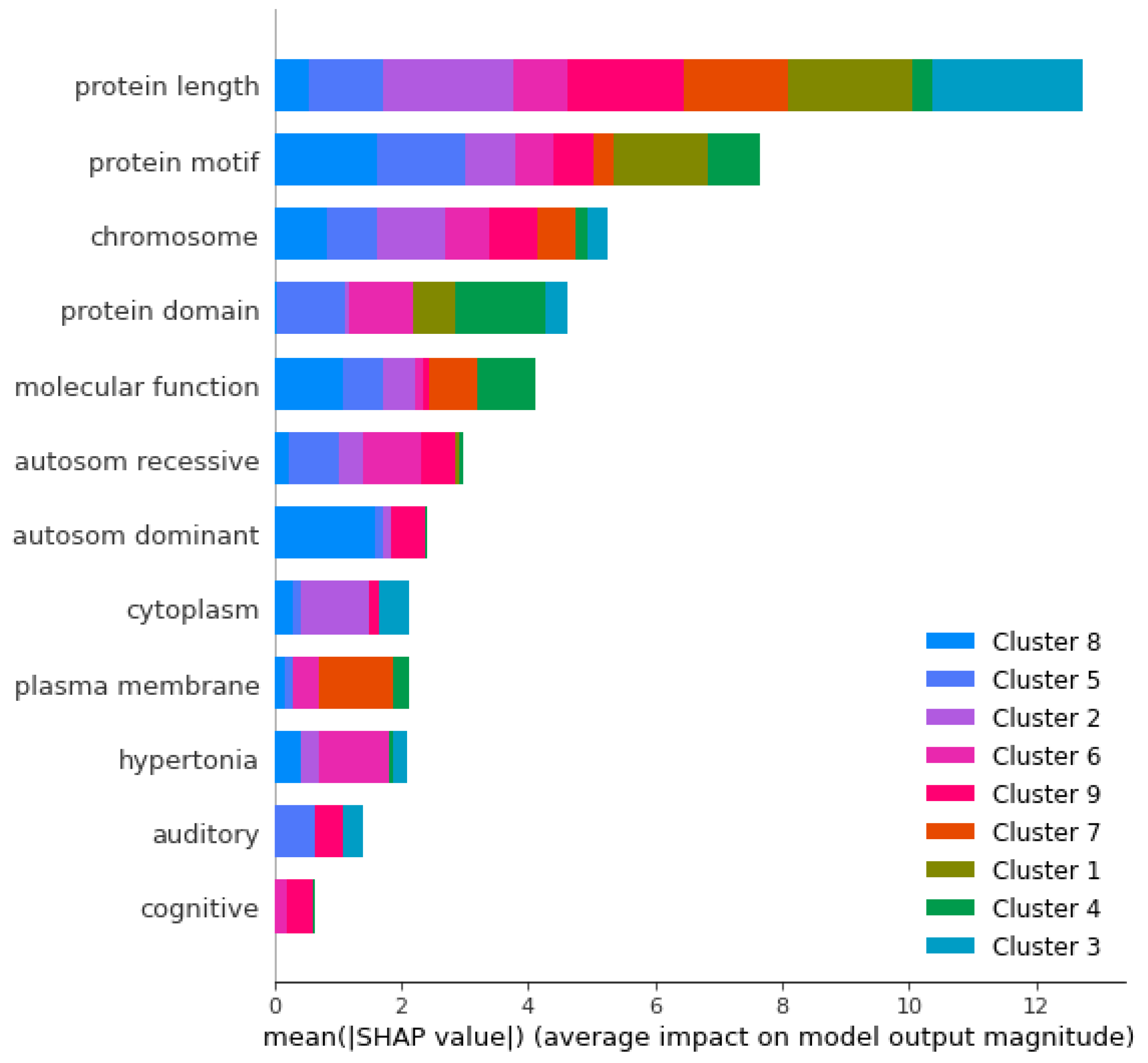
SHAP summary values were calculated using the method of Lundberg et al. [68]. START cluster membership was added to the flattened feature array (see above). The cluster configuration was fitted to the HistGradientBoostingClassifier (scikit-learn). The shap. TreeExplainer and the shap.summary_plot procedures were used to compute SHAP values and create the SHAP summary plot.

5. Results

5.1. Selection of Cluster Configuration for the CMT Dataset

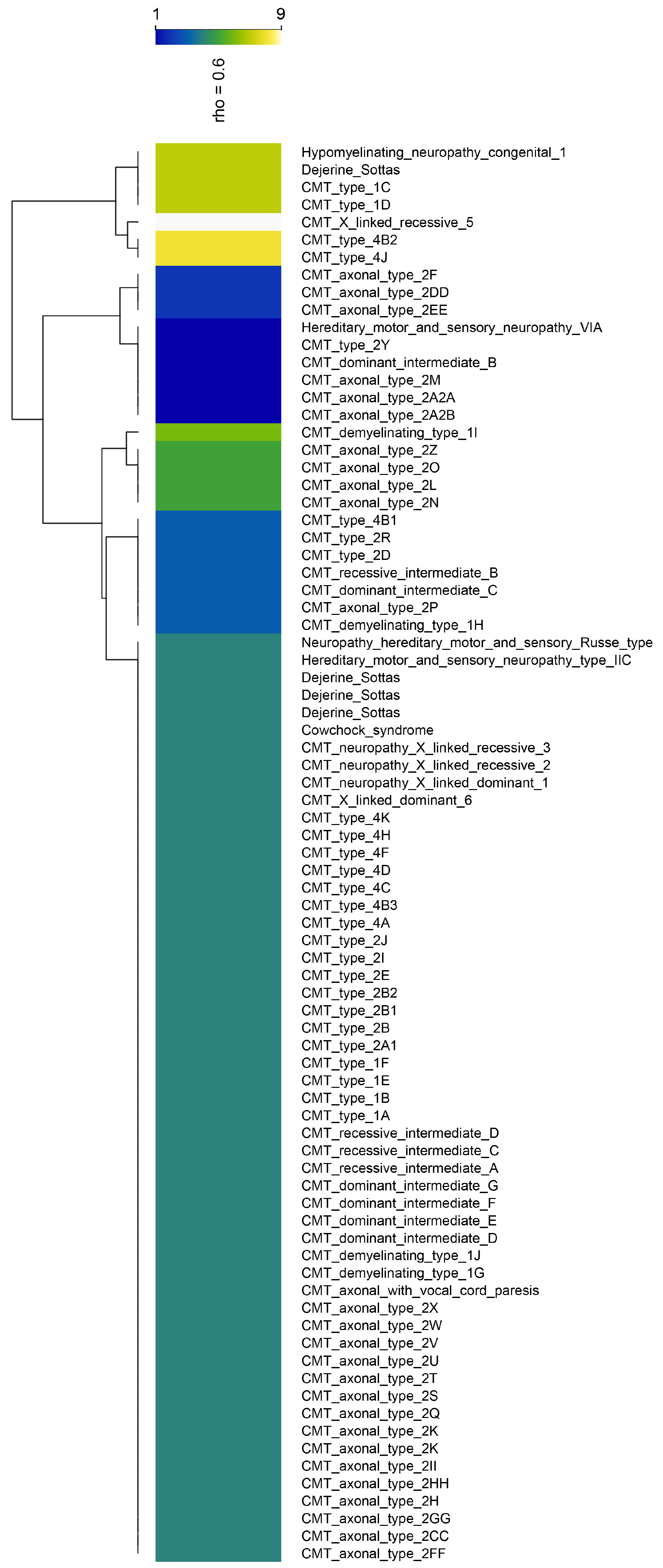
The vigilance parameter ρ was varied between 0.0 and 1.0 in a Monte Carlo of shuffled sample presentation order (Figure 3). To minimize the size of the largest cluster and minimize the number of clusters with one member, ρ = 0.6 was selected, yielding nine clusters (Figure 4).

5.2. Cluster Characterization by Feature Composition

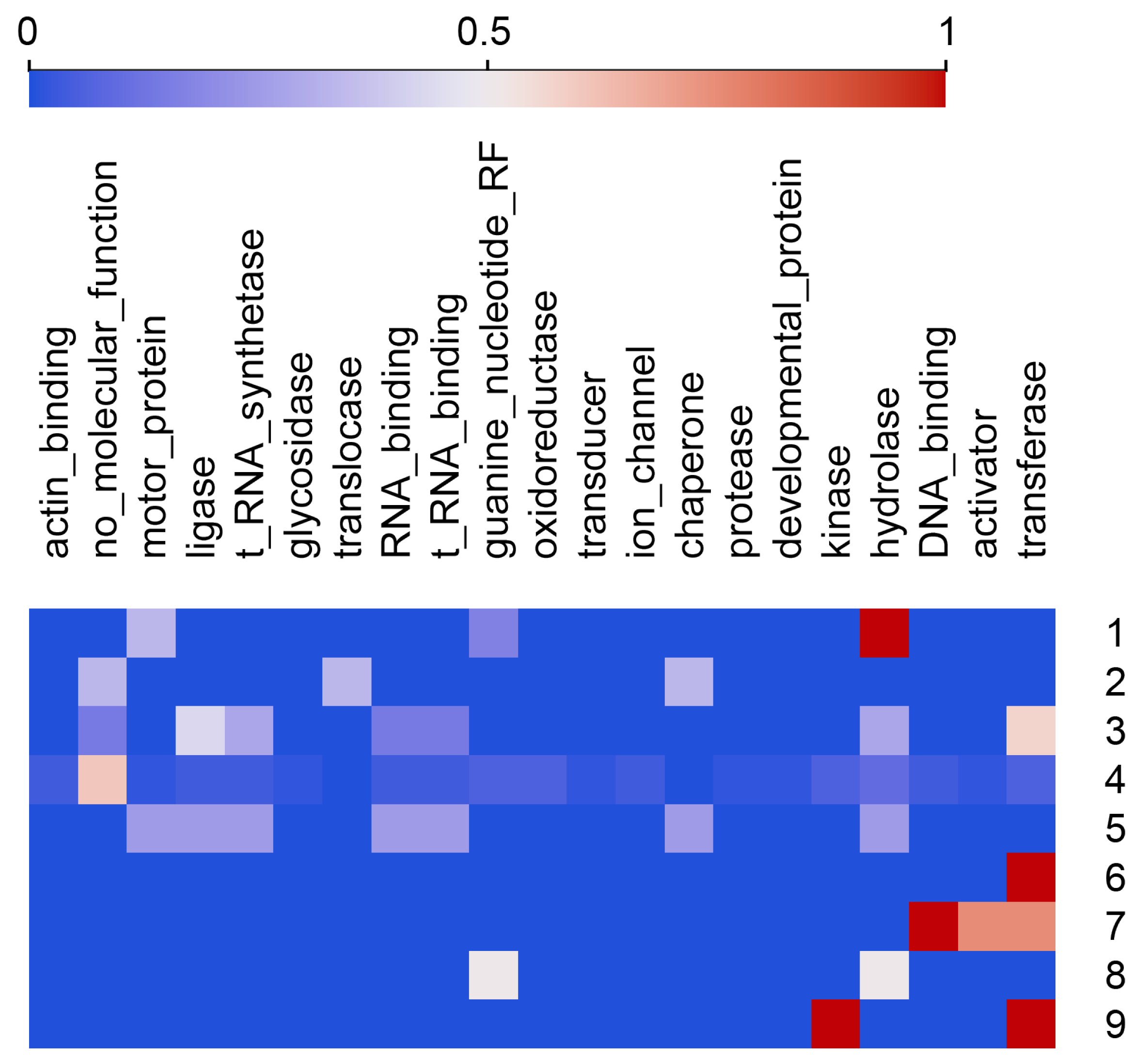
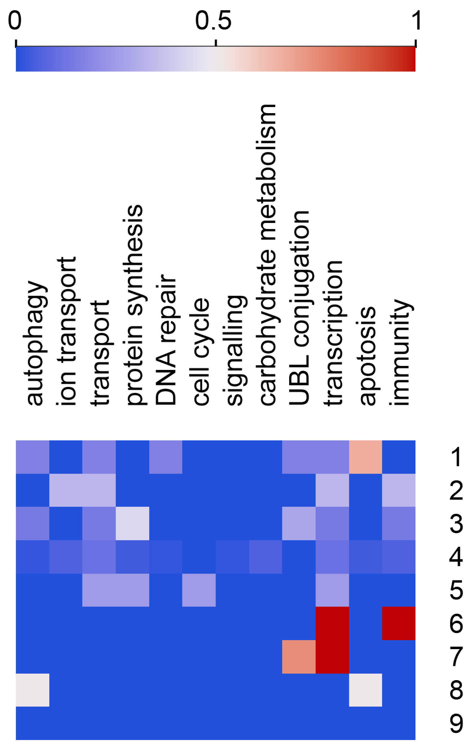
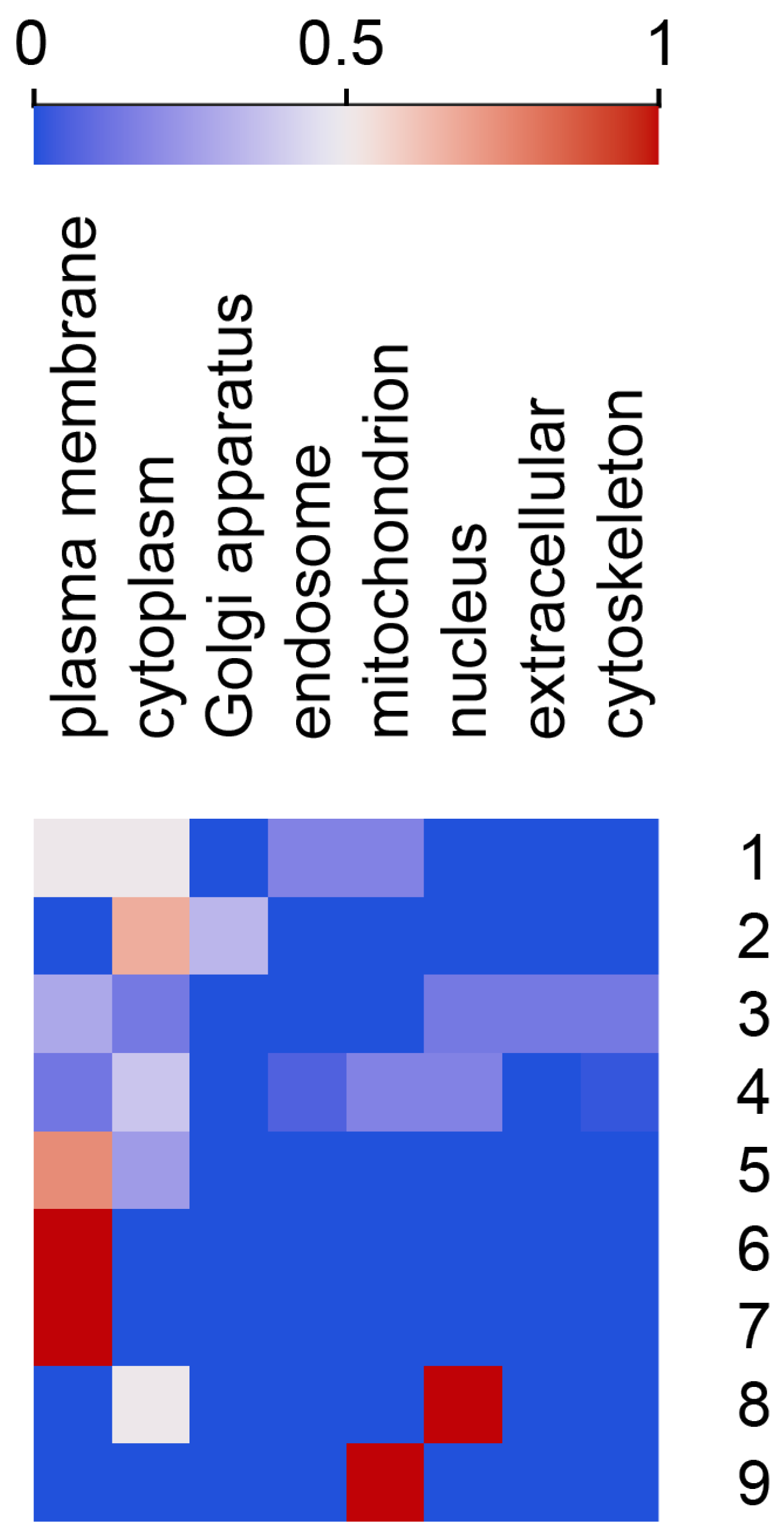
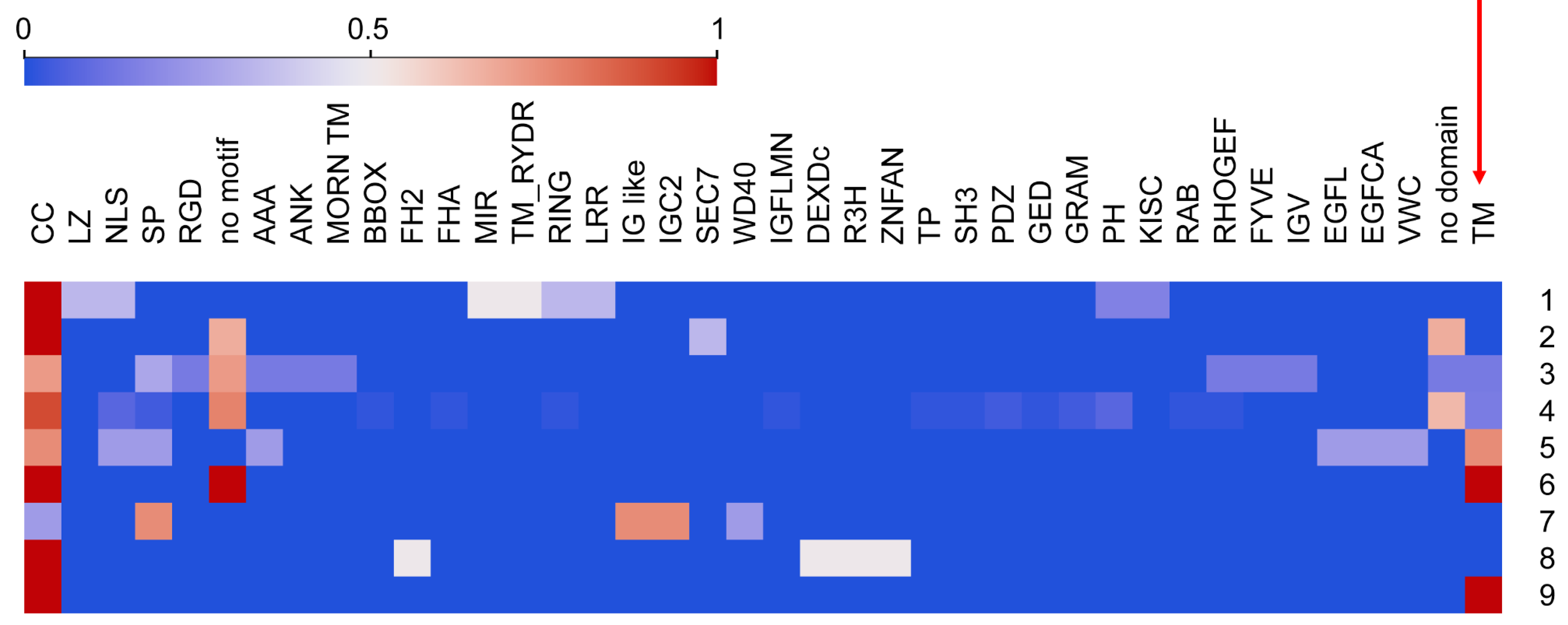
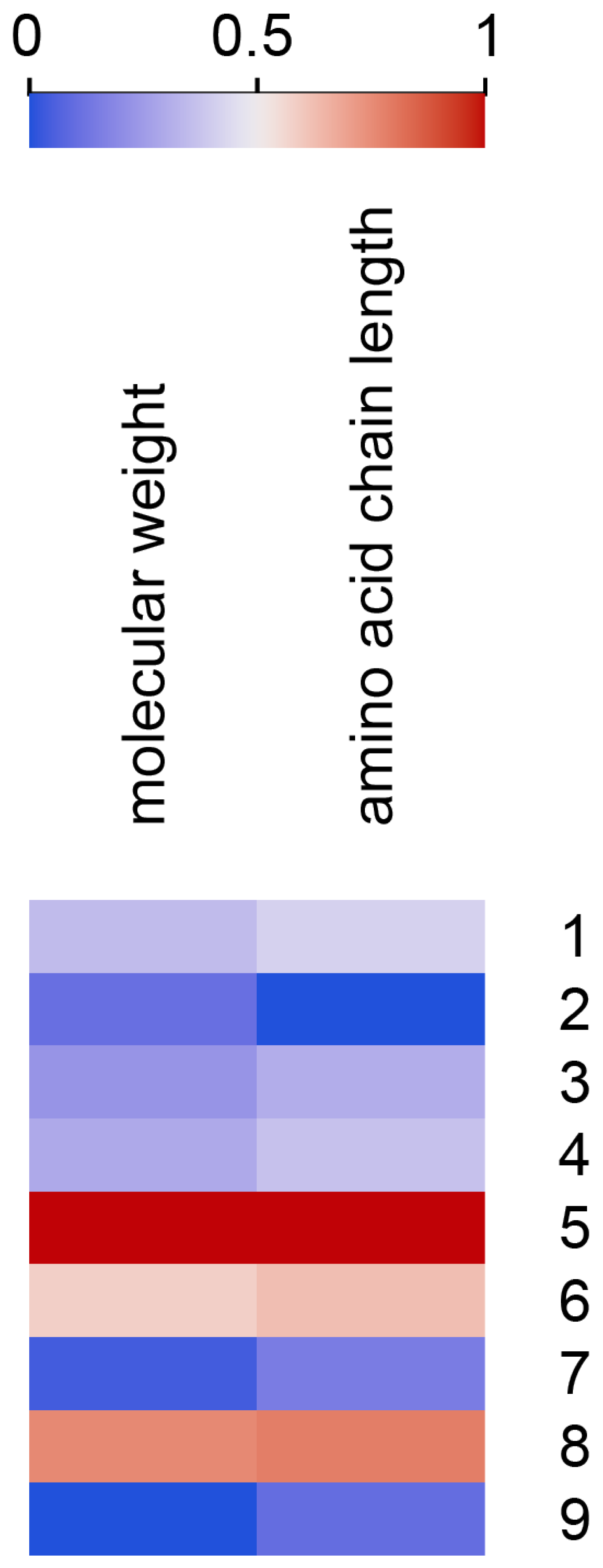
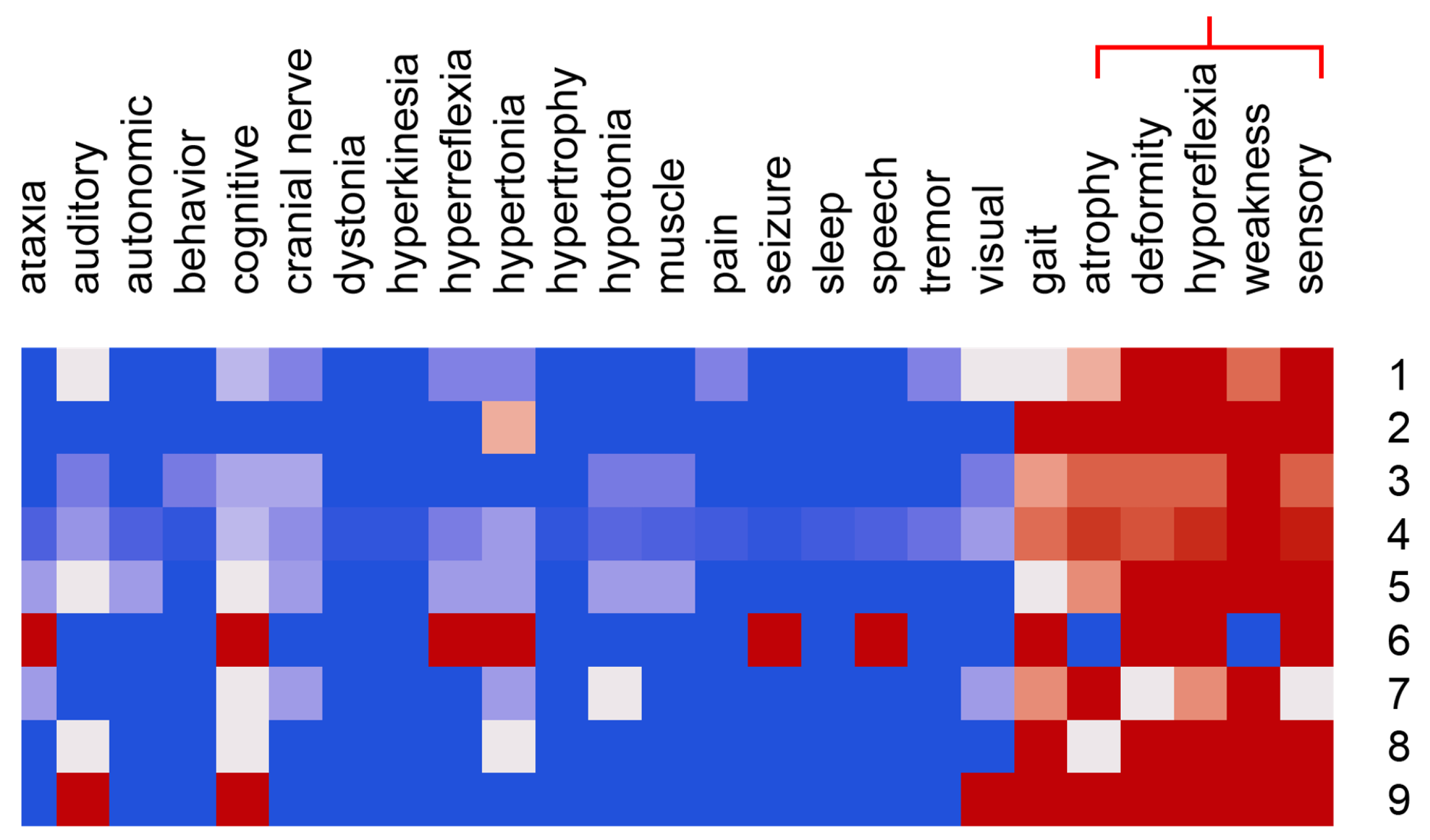
We used heat maps to visualize the features that characterized each cluster. The clusters differed in mode of inheritance, protein localization within the cell, protein participation in biological processes, protein length, molecular weight, motifs and domains in amino acid chains, phenotype, and protein molecular function (Figure 5, Figure 6, Figure 7, Figure 8, Figure 9, Figure 10, Figure 11 and Figure 12). The heat maps were used to create a narrative summary of each cluster’s most important feature characteristics (Table 7).

5.3. Identifying Features That Contributed the Most to Cluster Configuration

We used SHAP [68] to find the features that drove the cluster configuration. The SHAP summary plot (Figure 12) showed that protein length, chromosome number (autosomes 1 22 and X and Y), mode of inheritance (autosomal recessive and autosomal dominant), protein localization in the cell (cytoplasm and plasma membrane), and phenotype (hypertonia, auditory and cognitive) contributed the most to cluster formation.

6. Discussion

6.1. Feasibility of Clustering Multi-Categorical Biomedical Data with START

START demonstrates several important capabilities that make it particularly useful for the clustering of multi-categorical data. Firstly, it directly represents the categorical data without an intermediate encoding representation and all the problems introduced therein; categorical data by definition does not define distance metrics or fuzzy membership between categories and feature dimensions. The problem is circumvented here by the definition of prototype parse trees tracking the distributions of symbols from learned statements using the ART match and learning rules.
Secondly, it naturally compensates for data points with missing elements entries in its fields; rather than requiring a special encoding scheme for missing fields or removing data points altogether, START can represent missing fields as unused non-terminal positions when representing multi-categorical datasets as statements containing one or more attributes, which has the effect of penalizing the degree to which samples with missing features match existing prototypes while still accommodating prototypes of varying sizes.
Thirdly, and as a consequence of the previous point, START can handle symbolic data of varying length when interpreted as statements under a grammar; in fact, this paper demonstrates an analysis of multi-categorical datasets of depth 2 due to the nature of the CMT data available, but categorical datasets of arbitrary depth can be analyzed with START when treating categories as themselves non-terminal symbols with production rules mapping to other sets of categories. This can be interpreted as processing hierarchical symbolic databases where individual fields can themselves link to other symbolic database tables.

6.2. Biological Interest and Plausibility of Derived Clusters

When the START vigilance parameter was set to ρ = 0.6 (Figure 3), we obtained nine clusters (Table 7). Cluster 4, the largest, had 53 members, and clusters 6 and 9 were singleton clusters. The fact that cluster 4 is large is not surprising since most cases of CMT are similar and have similar core symptoms of weakness, sensory loss, hyporeflexia, orthopedic abnormalities, atrophy, and gait abnormalities in common [76]. Although it is usual to differentiate clinically between axonal forms (involving the neuron axon) and demyelinating forms (involving the myelin sheath of the axon) of CMT, it is not surprising that we did not find axonal and demyelinating clusters of CMT since we did not input electromyographic data into the clustering algorithm. The finding of small clusters of CMT variants with auditory, hypertonic, or cognitive phenotypes is interesting and plausible biologically and is consistent with clinical observations.
The clusters differed in inheritance (Table 7) in biologically plausible ways and consistent with clinical practice. Since each variant of CMT was due to a gene mutation and since each gene coded for a unique protein, protein weight, protein length, protein configuration (motifs and domains), protein involvement in biological processes, protein molecular function, and protein locations could be examined for each CMT cluster and compared to the observed phenotype (Figure 5, Figure 6, Figure 7, Figure 8, Figure 9, Figure 10, Figure 11 and Figure 12, and Table 7). Although these observations are intriguing, they do not offer a precise path to connect protein function, location, and process to the neurological phenotype in CMT. As an example of explainable AI [82], the SHAP plots in Figure 12 provide biologically plausible explanations for how START relied on certain features to form clusters.

6.3. Limitations

One limitation of this work is that START is used to cluster a small biomedical dataset without ground truth labeling. Although the diagnosis of each row (CMT disease variant) is known, cluster membership for the dataset as a whole is unknown. As a result, this work cannot contain an analysis of either truth in cluster membership and structure or performance of START with respect to such a ground truth. The reader is referred to the Supplementary Materials of this article for a study of the START algorithm on various other machine learning benchmark datasets, including fully symbolic and real-valued datasets including details of the procedure necessary to adapt the START algorithm to real-valued data.
Another limitation of this work is that all available features are used as inputs to the START clustering algorithm. A separate study is warranted to study how withholding some of the features as meta-features would allow potentially interesting cluster composition analyses.
Furthermore, the results of clustering and analyzing the CMT dataset with START has limited generalizability to other diseases datasets. It is seldom expected of clustering models or indeed machine learning models as a whole to generalize to distinct domains from which they were trained, outside of research areas such as lifelong machine learning that tackle this specific issue [83]. Nevertheless, some transferability should be expected to related datasets of the class of neurogenetic diseases that CMT belongs to, but this transferability is limited in two ways: by the format of the selected data and the START methodology itself. Biomedical data are themselves notoriously multifaceted, and the creation of generalizing models in this field depends on the narrowed problem statement and subsequent dataset at hand. For example, this work considers the clustering of data with categorical membership in specifically phenotype–gene relationships; with respect to the OMIM elements, each entry in the CMT dataset subsumes a variable number of clinical studies that generate the datapoints, discarding the qualitative aspects of the various individuals studied and the other clinical features that are inconsistently included between entries. This is a consequence not of the quality of the OMIM database but rather of the project of aggregating vastly disparate clinical data.
In addition to this, an ontological level of granularity is necessarily selected by the researcher when working with any clinical features; for example, a full hierarchy of pain may be studied as symptoms of a disease with respect to an individual patient from the location, duration/periodicity, and subjective intensity according to some pain scale, etc. Taking the location of pain as an example, some studies describe the location of pain with a varying degree of specificity; in the hierarchy of location on the human body, should one hypothetical study citing simply pain and another citing leg pain be considered the same by virtue of belonging on the same hierarchy or different by virtue of being two different points on that hierarchy? If neither is true, then what is the distance metric along this hierarchy until two points are considered distinct? Even clinical definitions of the term pain itself vary and are subject to debate [84]. As a result, simplifying assumptions must be made for any learned model of clinical data, such as the ontological subsumption of the phenotype of pain in this study, and the interpretation of clustering results and its usefulness for the treatment of a disease is tied to the selection of ontological granularity.
Lastly, the methodology of the START algorithm successfully tackles the clustering of the resulting variable-size categorical datasets, but it does so at the level of the symbols themselves without forming a feature-transformed intermediate representation of them. Additional similar phenotype–gene datasets could be clustered with an existing model trained on this CMT dataset, but relationships between them would only be found if they shared exactly the same symbols, such as gene locations and disease phenotypes. Completely disparate datasets with no shared symbols may indeed be clustered by the same START model after appropriate modifications to its parser’s grammar, but this would be functionally equivalent to clustering with two separate START models; this benefit of START is also to its detriment, as if there are no shared symbols between data points, they are treated as having no shared features for computing similarities.

6.4. Future Work

This paper demonstrates that START can work with data from a knowledge graph or ontology when flattened into a rectangular file, even with missing or nested elements. Alternatively, knowledge graphs and ontologies can be converted into triplets as subject–object–predicate triplets, which retains the underlying graph architecture. In the future, we plan to determine whether START can successfully cluster these triplets derived from knowledge graphs into meaningful clusters.
Additional future work includes an evaluation of START clustering on large multi-categorical datasets with a known ground truth cluster membership and further experiments on datasets in which some features are withheld from input and retained as meta-features for post-clustering analysis.

7. Conclusions

This work introduces the START algorithm for the clustering of symbolic data with arbitrary length statements. This work also introduces dual-vigilance and distributed dual-vigilance variants of START along with a supervised modification for each. Because START is designed for symbolic datasets, it is naturally suited for the clustering of both categorical and multi-categorical datasets where each sample feature may realize multiple values. This multi-categorical clustering capability is demonstrated on a curated biomedical dataset of Charcot–Marie–Tooth disease variants and their disease–gene attributes, such as disease phenotypes and protein molecular functions.
For a dataset such as the CMT dataset used here, START is useful as a tool for studying structural relationships between disease variants for guiding future clinical research or in the formulation of useful models of those diseases via the hierarchies, clusters, and outliers identified during the clustering process; for example, distinct gene locations with shared phenotypes between two groups of disease variants may illustrate to a researcher some other shared molecular mechanism for future research, which could guide drug research in a data-driven manner.

Supplementary Materials

The following supporting information can be downloaded at: https://www.mdpi.com/article/10.3390/info15030125/s1, Listing S1: Discretized Iris dataset grammar illustrating the symbolic binning procedure of real-valued data used to evaluate START and Gram-ART; Table S1: Hyperparameters for each START variant during supervised train/test evaluation. Table S2: Performance statistics of the supervised implementations of each START variant derived in the original paper on a set of benchmark real-valued and categorical machine learning datasets.

Author Contributions

Conceptualization, D.B.H., S.P. and D.C.W.II; methodology, S.P. and D.B.H.; software, S.P. and D.B.H.; validation, S.P.; formal analysis, S.P. and D.B.H.; investigation, S.P. and D.B.H.; resources, D.B.H. and D.C.W.II; data curation, D.B.H.; writing—original draft preparation, S.P. and D.B.H.; writing—review and editing, S.P., D.B.H., T.O.-A., M.A.B., E.J.T., W.E.M., M.S. and D.C.W.II; visualization, S.P. and D.B.H.; supervision, D.C.W.II; project administration, D.C.W.II and E.J.T.; funding acquisition, S.P. and D.C.W.II. All authors have read and agreed to the published version of the manuscript.

Funding

This work is funded by the Department of Energy’s Kansas City National Security Campus, operated by Honeywell Federal Manufacturing & Technologies, LLC, under contract number DE-NA0002839.

Institutional Review Board Statement

Not applicable.

Informed Consent Statement

Not applicable.

Data Availability Statement

Disease–protein datasets are gathered from the openly available Online Mendelian Inheritance in Man (OMIM) knowledge base [85]. All data, code, and documentation related to the experiments outlined in this paper are contained in a version-archived repository [66].

Conflicts of Interest

The authors declare no conflicts of interest.

Abbreviations

The following abbreviations are used in this manuscript:
ARTAdaptive resonance theory
BNFBackus–Naur form
CFGContext-free grammar
CMTCharcot–Marie–Tooth disease
DDVFADistributed dual-vigilance FuzzyART
DDV-STARTDistributed dual-vigilance symbolic tree adaptive resonance theory
DVFADual-vigilance FuzzyART
DV-STARTDual-vigilance symbolic tree adaptive resonance theory
EBNFExtended Backus–Naur form
F1ART Feature input layer (field 1)
F2ART Category representation layer (field 2)
HACHierarchical agglomerative clustering
L2Lifelong learning
MLMachine learning
PMFProbability mass function
START          Symbolic tree ART
WTAWinner-take-all

Appendix A. Charcot–Marie–Tooth Dataset Grammar

An analysis of the Charcot–Marie–Tooth (CMT) dataset a posteriori demonstrates the process used in this article for interpreting tabular multi-categorical data as statements sampled from a context-free grammar that can be expressed as a set of EBNF production rules, which can be seen in Grammar Listing 1. Gene–protein disease data are gathered for 81 variants of CMT with categorical attributes (Table 6). Categories such as phenotype are subsumed where hierarchically relevant to reduce attribute feature dimensionality (e.g., variants of “pain" symptomology are subsumed to one feature belonging to the “phenotype" attribute). This process results in a 81-row flat-file dataset of features with multi-categorical attributes represented as piped entries for each disease variant, including attributes with missing entries.

References

  1. Robinson, P.N. Deep phenotyping for precision medicine. Hum. Mutat. 2012, 33, 777–780. [Google Scholar] [CrossRef]
  2. Sonawane, A.R.; Weiss, S.T.; Glass, K.; Sharma, A. Network medicine in the age of biomedical big data. Front. Genet. 2019, 10, 294. [Google Scholar] [CrossRef]
  3. Collins, F.S.; Varmus, H. A new initiative on precision medicine. N. Engl. J. Med. 2015, 372, 793–795. [Google Scholar] [CrossRef]
  4. Carrasco-Ramiro, F.; Peiró-Pastor, R.; Aguado, B. Human genomics projects and precision medicine. Gene Ther. 2017, 24, 551–561. [Google Scholar] [CrossRef]
  5. Phillips, C.J. Precision medicine and its imprecise history. Harv. Data Sci. Rev. 2020, 2, 1–10. [Google Scholar]
  6. Ginsburg, G.S.; Phillips, K.A. Precision medicine: From science to value. Health Aff. 2018, 37, 694–701. [Google Scholar] [CrossRef] [PubMed]
  7. Polster, A.; Cvijovic, M. Network medicine: Facilitating a new view on Complex Diseases. Front. Bioinform. 2023, 3, 47. [Google Scholar]
  8. Healy, M.J.; Caudell, T.P. Ontologies and worlds in category theory: Implications for neural systems. Axiomathes 2006, 16, 165–214. [Google Scholar] [CrossRef]
  9. Bezdek, J.C. Elementary Cluster Analysis: Four Basic Methods That (Usually) Work; River Publishers: Gistrup, Denmark, 2022. [Google Scholar]
  10. Xu, R.; Wunsch, D.C. Clustering; John Wiley & Sons, Inc.: Hoboken, NJ, USA, 2009; pp. 1–21. [Google Scholar]
  11. Gowda, K.; Diday, E. Symbolic clustering using a new similarity measure. IEEE Trans. Syst. Man Cybern. 1992, 22, 368–378. [Google Scholar] [CrossRef]
  12. Chidananda Gowda, K.; Diday, E. Symbolic clustering using a new dissimilarity measure. Pattern Recognit. 1991, 24, 567–578. [Google Scholar] [CrossRef]
  13. Carpenter, G.A.; Grossberg, S. The ART of adaptive pattern recognition by a self-organizing neural network. Computer 1988, 21, 77–88. [Google Scholar] [CrossRef]
  14. Carpenter, G.A.; Grossberg, S.; Markuzon, N.; Reynolds, J.H.; Rosen, D.B. Fuzzy ARTMAP: A neural network architecture for incremental supervised learning of analog multidimensional maps. IEEE Trans. Neural Netw. 1992, 3, 698–713. [Google Scholar] [CrossRef] [PubMed]
  15. Tan, A.H. Adaptive resonance associative map. Neural Netw. 1995, 8, 437–446. [Google Scholar] [CrossRef]
  16. Subagdja, B.; Tan, A.H. iFALCON: A neural architecture for hierarchical planning. Neurocomputing 2012, 86, 124–139. [Google Scholar] [CrossRef]
  17. Subagdja, B.; Tan, A.H. Planning with iFALCON: Towards a neural-network-based BDI agent architecture. In Proceedings of the 2008 IEEE/WIC/ACM International Conference on Web Intelligence and Intelligent Agent Technology, Sydney, Australia, 9–12 December 2008; IEEE: Los Alamitos, CA, USA, 2008; Volume 2, pp. 231–237. [Google Scholar]
  18. Kim, T.; Hwang, I.; Lee, H.; Kim, H.; Choi, W.S.; Lim, J.J.; Zhang, B.T. Message passing adaptive resonance theory for online active semi-supervised learning. In Proceedings of the International Conference on Machine Learning. PMLR, Virtual, 18–24 July 2021; pp. 5519–5529. [Google Scholar]
  19. Brito da Silva, L.E.; Elnabarawy, I.; Wunsch, D.C. A Survey of Adaptive Resonance Theory Neural Network Models for Engineering Applications. Neural Netw. 2019, 120, 167–203. [Google Scholar] [CrossRef]
  20. Carpenter, G.A.; Grossberg, S.; Rosen, D.B. Fuzzy ART: Fast stable learning and categorization of analog patterns by an adaptive resonance system. Neural Netw. 1991, 4, 759–771. [Google Scholar] [CrossRef]
  21. Bezdek, J.C.; Keller, J.; Krisnapuram, R.; Pal, N. Fuzzy Models and Algorithms for Pattern Recognition and Image Processing; Springer Science & Business Media: New York, NY, USA, 1999; Volume 4. [Google Scholar]
  22. Ruspini, E.H.; Bezdek, J.C.; Keller, J.M. Fuzzy clustering: A historical perspective. IEEE Comput. Intell. Mag. 2019, 14, 45–55. [Google Scholar] [CrossRef]
  23. Keller, J.M.; Yager, R.R.; Tahani, H. Neural network implementation of fuzzy logic. Fuzzy Sets Syst. 1992, 45, 1–12. [Google Scholar] [CrossRef]
  24. Meuth, R.J. Adaptive Multi-Vehicle Mission Planning for Search Area Coverage. Ph.D. Thesis, Missouri University of Science and Technology, Rolla, MO, USA, 2007. [Google Scholar]
  25. Brito da Silva, L.E.; Elnabarawy, I.; Wunsch, D.C. Dual vigilance fuzzy adaptive resonance theory. Neural Netw. 2019, 109, 1–5. [Google Scholar] [CrossRef]
  26. Brito da Silva, L.E.; Elnabarawy, I.; Wunsch, D.C. Distributed dual vigilance fuzzy adaptive resonance theory learns online, retrieves arbitrarily-shaped clusters, and mitigates order dependence. Neural Netw. 2020, 121, 208–228. [Google Scholar] [CrossRef]
  27. Grossberg, S. How Does a Brain Build a Cognitive Code? Psychol. Rev. 1980, 87, 1–51. [Google Scholar] [CrossRef] [PubMed]
  28. Grossberg, S.; Grossberg, S. How does a brain build a cognitive code? In Studies of Mind and Brain: Neural Principles of Learning, Perception, Development, Cognition, and Motor Control; Springer: Dordrecht, The Netherlands, 1982; pp. 1–52. [Google Scholar]
  29. Cohen, M.A.; Grossberg, S. Absolute stability of global pattern formation and parallel memory storage by competitive neural networks. IEEE Trans. Syst. Man Cybern. 1983, SMC-13, 815–826. [Google Scholar] [CrossRef]
  30. Grossberg, S. Nonlinear neural networks: Principles, mechanisms, and architectures. Neural Netw. 1988, 1, 17–61. [Google Scholar] [CrossRef]
  31. Grossberg, S.T. Studies of Mind and Brain: Neural Principles of Learning, Perception, Development, Cognition, and Motor Control; Boston Studies in the Philosophy and History of Science Springer Dordrecht: Dordrecht, Holland, 1982; Volume 70. [Google Scholar]
  32. Grossberg, S.; Versace, M. Spikes, synchrony, and attentive learning by laminar thalamocortical circuits. Brain Res. 2008, 1218, 278–312. [Google Scholar] [CrossRef] [PubMed]
  33. Grossberg, S. Adaptive Resonance Theory: How a brain learns to consciously attend, learn, and recognize a changing world. Neural Netw. 2013, 37, 1–47. [Google Scholar] [CrossRef] [PubMed]
  34. Grossberg, S. The resonant brain: How attentive conscious seeing regulates action sequences that interact with attentive cognitive learning, recognition, and prediction. Atten. Percept. Psychophys. 2019, 81, 2237–2264. [Google Scholar] [CrossRef]
  35. Grossberg, S. Conscious Mind, Resonant Brain: How Each Brain Makes a Mind; Oxford University Press: Oxford, UK, 2021. [Google Scholar] [CrossRef]
  36. Carpenter, G.A.; Grossberg, S. A massively parallel architecture for a self-organizing neural pattern recognition machine. Comput. Vis. Graph. Image Process. 1987, 37, 54–115. [Google Scholar] [CrossRef]
  37. Carpenter, G.A.; Grossberg, S. Pattern Recognition by Self-Organizing Neural Networks; The MIT Press: Cambridge, MA, USA, 1991. [Google Scholar]
  38. Carpenter, G.; Grossberg, S. Adaptive Resonance Theory; Technical report; Boston University Center for Adaptive Systems and Department of Cognitive and Neural Systems: Boston, MA, USA, 1998. [Google Scholar]
  39. Petrenko, S.; Wunsch, D.C. AdaptiveResonance.jl: A Julia Implementation of Adaptive Resonance Theory (ART) Algorithms. J. Open Source Softw. 2022, 7, 3671. [Google Scholar] [CrossRef]
  40. Park, G.M.; Kim, J.H. Deep Adaptive Resonance Theory for learning biologically inspired episodic memory. In Proceedings of the 2016 International Joint Conference on Neural Networks (IJCNN), Vancouver, BC, Canada, 24–29 July 2016; pp. 5174–5180. [Google Scholar] [CrossRef]
  41. Carpenter, G.A. Distributed learning, recognition, and prediction by ART and ARTMAP neural networks. Neural Netw. 1997, 10, 1473–1494. [Google Scholar] [CrossRef]
  42. Carpenter, G.A.; Milenova, B.L.; Noeske, B.W. Distributed ARTMAP: A neural network for fast distributed supervised learning. Neural Netw. 1998, 11, 793–813. [Google Scholar] [CrossRef] [PubMed]
  43. Healy, M.J.; Caudell, T.P.; Smith, S.D. A neural architecture for pattern sequence verification through inferencing. IEEE Trans. Neural Netw. 1993, 4, 9–20. [Google Scholar] [CrossRef]
  44. Grossberg, S.; Huang, T.R. ARTSCENE: A neural system for natural scene classification. J. Vis. 2009, 9, 6. [Google Scholar] [CrossRef] [PubMed]
  45. Petrenko, S.; Brna, A.; Aguilar-Simon, M.; Wunsch, D. Lifelong Context Recognition via Online Deep Feature Clustering. TechRxiv 2023, 14, 1–15. [Google Scholar] [CrossRef]
  46. Brna, A.P.; Brown, R.C.; Connolly, P.M.; Simons, S.B.; Shimizu, R.E.; Aguilar-Simon, M. Uncertainty-based modulation for lifelong learning. Neural Netw. 2019, 120, 129–142. [Google Scholar] [CrossRef]
  47. Brown, R.; Brna, A.; Cook, J.; Park, S.; Aguilar-Simon, M. Uncertainty-Driven Control for a Self-Supervised Lifelong Learning Drone. In Proceedings of the IGARSS 2022—2022 IEEE International Geoscience and Remote Sensing Symposium, Kuala Lumpur, Malaysia, 17–22 July 2022; pp. 5053–5056. [Google Scholar] [CrossRef]
  48. Aguilar-Simon, M.; Brna, A.; Brown, R.; Folsom, L.; Cook, J.; Park, S.; Yanoschak, A.; Shimizu, R.; Scientific, T.; Imaging, L. Adaptive Learning Through Active Neuromodulation (ALAN); Air Force Research Laboratory, Sensors Directorate: Wright-Patterson Air Force Base, OH, USA, 2022. [Google Scholar]
  49. Petrenko, S.; Wunsch, D.C. ClusterValidityIndices.jl: Batch and Incremental Metrics for Unsupervised Learning. J. Open Source Softw. 2022, 7, 3527. [Google Scholar] [CrossRef]
  50. Brito da Silva, L.E.; Rayapati, N.; Wunsch, D.C. Incremental Cluster Validity Index-Guided Online Learning for Performance and Robustness to Presentation Order. IEEE Trans. Neural Netw. Learn. Syst. 2022, 34, 6686–6700. [Google Scholar] [CrossRef]
  51. Brito da Silva, L.E.; Rayapati, N.; Wunsch, D.C. iCVI-ARTMAP: Using Incremental Cluster Validity Indices and Adaptive Resonance Theory Reset Mechanism to Accelerate Validation and Achieve Multiprototype Unsupervised Representations. IEEE Trans. Neural Netw. Learn. Syst. 2022, 34, 1–14. [Google Scholar] [CrossRef]
  52. Yelugam, R.; Brito da Silva, L.E.; Wunsch, D.C. TopoBARTMAP: Biclustering ARTMAP with or without Topological Methods in a Blood Cancer Case Study. In Proceedings of the 2020 International Joint Conference on Neural Networks (IJCNN), Virtual, 19–24 July 2020; pp. 1–8. [Google Scholar] [CrossRef]
  53. Yelugam, R.; Brito da Silva, L.E.; Wunsch II, D.C. Topological biclustering ARTMAP for identifying within bicluster relationships. Neural Netw. 2023, 160, 34–49. [Google Scholar] [CrossRef]
  54. Some new indexes of cluster validity. IEEE Trans. Syst. Man Cybern. Part B (Cybern.) 1998, 28, 301–315. [CrossRef]
  55. Chen, Z.; Liu, B. Lifelong Machine Learning; Morgan & Claypool Publishers: San Rafael, CA, USA, 2018; pp. 1–207. [Google Scholar]
  56. Kudithipudi, D.; Aguilar-Simon, M.; Babb, J.; Bazhenov, M.; Blackiston, D.; Bongard, J.; Brna, A.P.; Chakravarthi Raja, S.; Cheney, N.; Clune, J.; et al. Biological underpinnings for lifelong learning machines. Nat. Mach. Intell. 2022, 4, 196–210. [Google Scholar] [CrossRef]
  57. Baker, M.M.; New, A.; Aguilar-Simon, M.; Al-Halah, Z.; Arnold, S.M.; Ben-Iwhiwhu, E.; Brna, A.P.; Brooks, E.; Brown, R.C.; Daniels, Z.; et al. A domain-agnostic approach for characterization of lifelong learning systems. Neural Netw. 2023, 160, 274–296. [Google Scholar] [CrossRef]
  58. Chomsky, N. Syntactic Structures; Mouton: Oxford, UK, 1957. [Google Scholar]
  59. Chomsky, N. On the Notion" Rule of Grammar"; American Mathematical Society: Providence, RI, USA, 1961. [Google Scholar]
  60. Wolpert, D.; Macready, W. No free lunch theorems for optimization. IEEE Trans. Evol. Comput. 1997, 1, 67–82. [Google Scholar] [CrossRef]
  61. ISO/IEC 14977:1996 (E); Information Technology-Syntactic Metalanguage-Extended BNF. ISO/IEC: Geneva, Switzerland, 1996.
  62. Hester, J.R.; Shinan, E. Lerche: Generating data file processors in Julia from EBNF grammars. J. Open Source Softw. 2021, 6, 3497. [Google Scholar] [CrossRef]
  63. Carpenter, G.A.; Grossberg, S.; Reynolds, J.H. ARTMAP: Supervised real-time learning and classification of nonstationary data by a self-organizing neural network. In Proceedings of the IEEE Conference on Neural Networks for Ocean Engineering, Miami, FL, USA, 9–11 December 1991; pp. 341–342. [Google Scholar] [CrossRef]
  64. Kasuba, T. Simplified Fuzzy ARTMAP. AI Expert 1993, 8, 19–25. [Google Scholar]
  65. Tan, A.H. Cascade ARTMAP: Integrating neural computation and symbolic knowledge processing. IEEE Trans. Neural Netw. 1997, 8, 237–250. [Google Scholar]
  66. Petrenko, S. AP6YC/OAR: V0.1.0. Zenodo, 5 January 2024. [Google Scholar] [CrossRef]
  67. Bezanson, J.; Edelman, A.; Karpinski, S.; Shah, V.B. Julia: A fresh approach to numerical computing. SIAM Rev. 2017, 59, 65–98. [Google Scholar] [CrossRef]
  68. Lundberg, S.M.; Erion, G.; Chen, H.; DeGrave, A.; Prutkin, J.M.; Nair, B.; Katz, R.; Himmelfarb, J.; Bansal, N.; Lee, S.I. From local explanations to global understanding with explainable AI for trees. Nat. Mach. Intell. 2020, 2, 56–67. [Google Scholar] [CrossRef] [PubMed]
  69. Demšar, J.; Curk, T.; Erjavec, A.; Črt Gorup; Hočevar, T.; Milutinovič, M.; Možina, M.; Polajnar, M.; Toplak, M.; Starič, A.; et al. Orange: Data Mining Toolbox in Python. J. Mach. Learn. Res. 2013, 14, 2349–2353. [Google Scholar]
  70. Fisher, R.A. Iris; UCI Machine Learning Repository: Irvine, CA, USA, 1988. [Google Scholar] [CrossRef]
  71. Mushroom; UCI Machine Learning Repository: Irvine, CA, USA, 1987. [CrossRef]
  72. Lane, T. UNIX User Data; UCI Machine Learning Repository: Irvine, CA, USA, 1988. [Google Scholar] [CrossRef]
  73. Ilc, N. Datasets Package. Available online: https://www.researchgate.net/publication/239525861_Datasets_package (accessed on 5 January 2024).
  74. Fränti, P.; Sieranoja, S. K-Means Properties on Six Clustering Benchmark Datasets. Appl. Intell. 2018, 48, 4743–4759. [Google Scholar] [CrossRef]
  75. Ahmad, A.S.; Mayya, A.M. A new tool to predict lung cancer based on risk factors. Heliyon 2020, 6, e03402. [Google Scholar] [CrossRef] [PubMed]
  76. Rossor, A.M.; Polke, J.M.; Houlden, H.; Reilly, M.M. Clinical implications of genetic advances in Charcot–Marie–Tooth disease. Nat. Rev. Neurol. 2013, 9, 562–571. [Google Scholar] [CrossRef] [PubMed]
  77. Amberger, J.S.; Bocchini, C.A.; Scott, A.F.; Hamosh, A. OMIM.org: Leveraging knowledge across phenotype–gene relationships. Nucleic Acids Res. 2019, 47, D1038–D1043. [Google Scholar] [CrossRef]
  78. Köhler, S.; Gargano, M.; Matentzoglu, N.; Carmody, L.C.; Lewis-Smith, D.; Vasilevsky, N.A.; Danis, D.; Balagura, G.; Baynam, G.; Brower, A.M.; et al. The human phenotype ontology in 2021. Nucleic Acids Res. 2021, 49, D1207–D1217. [Google Scholar] [CrossRef] [PubMed]
  79. The UniProt Consortium. UniProt: The Universal Protein Knowledgebase in 2023. Nucleic Acids Res. 2023, 51, D523–D531. [Google Scholar] [CrossRef] [PubMed]
  80. Keshava Prasad, T.; Goel, R.; Kandasamy, K.; Keerthikumar, S.; Kumar, S.; Mathivanan, S.; Telikicherla, D.; Raju, R.; Shafreen, B.; Venugopal, A.; et al. Human protein reference database—2009 update. Nucleic Acids Res. 2009, 37, D767–D772. [Google Scholar] [CrossRef]
  81. Robinson, P.N.; Mungall, C.J.; Haendel, M. Capturing phenotypes for precision medicine. Mol. Case Stud. 2015, 1, a000372. [Google Scholar] [CrossRef]
  82. Gunning, D.; Stefik, M.; Choi, J.; Miller, T.; Stumpf, S.; Yang, G.Z. XAI—Explainable artificial intelligence. Sci. Robot. 2019, 4, eaay7120. [Google Scholar] [CrossRef]
  83. New, A.; Baker, M.; Nguyen, E.; Vallabha, G. Lifelong Learning Metrics. arXiv 2022, arXiv:2201.08278. [Google Scholar]
  84. Raja, S.N.; Carr, D.B.; Cohen, M.; Finnerup, N.B.; Flor, H.; Gibson, S.; Keefe, F.J.; Mogil, J.S.; Ringkamp, M.; Sluka, K.A.; et al. The revised International Association for the Study of Pain definition of pain: Concepts, challenges, and compromises. Pain 2020, 161, 1976–1982. [Google Scholar] [CrossRef]
  85. Hamosh, A.; Scott, A.F.; Amberger, J.S.; Bocchini, C.A.; McKusick, V.A. Online Mendelian Inheritance in Man (OMIM), a knowledgebase of human genes and genetic disorders. Nucleic Acids Res. 2005, 33, D514–D517. [Google Scholar] [CrossRef]
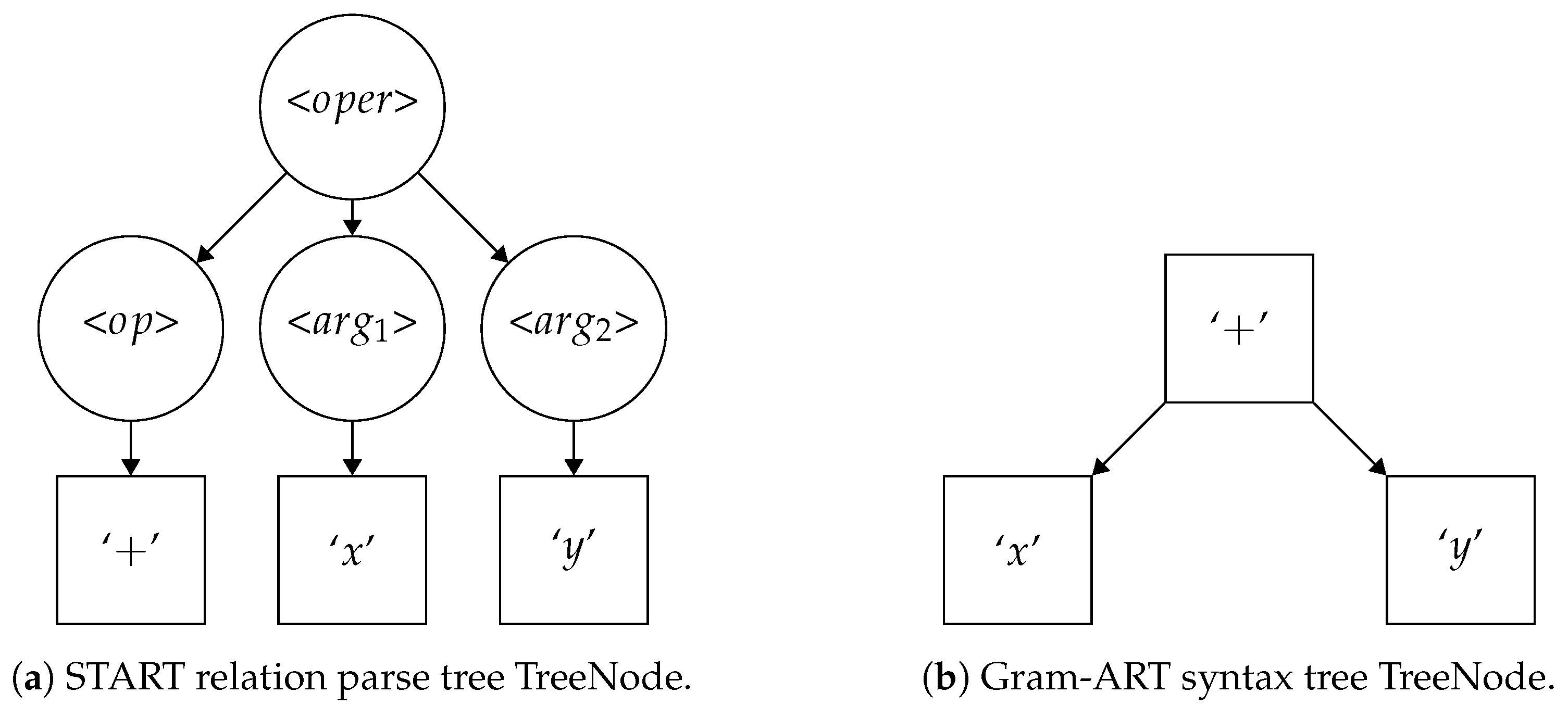
Figure 1. Comparison of the constituency relation parse trees of START (a) to the dependency parsing syntax trees of Gram-ART (b) for the simple algebraic statement x + y . START TreeNodes are full constituency relation parse trees containing terminal symbols at the leaves of the tree, while START ProtoNodes contain only non-terminal symbols at non-terminal positions on the parse tree. As in the Grammar Listing 1, non-terminal symbols are surrounded by arrows <·> and terminal symbols are in single quotations. Here, < o p e r > denotes “operation”, < o p > denotes “operator,” and < a r g 1 > and < a r g 2 > denote the two “arguments” of the operator.
Information 15 00125 g001
Figure 2. A set of figures demonstrating the evaluation and update of a START prototype on a new sample. (a (left)) demonstrates a START prototype as a rooted tree of ProtoNodes instantiated on the algebraic statement x + y (a). ProtoNodes are labeled by a non-terminal symbol, and they contain a probability mass function (PMF) of the terminal symbols generated both by that non-terminal and by any descendant non-terminals, where p x , y is shorthand for the PMF of the set of outcomes S = x 1 , x 2 , x n that gives p x 1 , x 2 , x n = P X = x | x S . (b (center)) demonstrates the relation parse tree of a new algebraic statement x + m · n . The rooted trees of the prototype and parsed statement are aligned and compared as a graph intersection at the non-terminal positions. The START match rule (Section 3.1.3) then determines the activation and match values of this graph intersection as a function of the PMFs at each non-terminal position and the terminal symbols at the leaf nodes of the sample, and the hypothetical prototype of (a) is selected from a pool of other candidate prototypes. (c (right)) demonstrates the prototype after update, accommodating the new non-terminal symbol positions of the sample and updating the PMFs at each non-terminal position according to the START weight update rule (Equations (3) and (4)).
Information 15 00125 g002
Figure 3. Effect of vigilance parameter ρ on number of clusters. A Monte Carlo of shuffled sample presentation order was run to generate 1 σ intervals of the results at each vigilance parameter value. As ρ was increased from 0.0 to 1.0 , the maximum cluster size decreased, the number of clusters increased, and the number of singleton clusters increased. A value of ρ = 0.6 (yellow dashed line) was selected to yield 9 clusters with only two singleton clusters. Larger ρ values gave too many singleton clusters, and smaller ones put too many cases into one cluster.
Information 15 00125 g003
Figure 4. With ρ = 0.6 , clustering by START yielded nine clusters from 81 variants of CMT. Each cluster is a different color on the heat map. Order of clusters on heat map is 7, 9, 8, 2, 1, 6, 5, 3, 4, with ordering by Euclidean distance between cluster centroids [69]. The largest cluster is 4 (dark green), with 53 members. Singleton clusters are 9 (white) and 6 (pea green). A shortened variant name is shown in the right margin. Dejerine–Sottas disease appears four times in the heat map because it is caused by four distinct mutations in the MPZ, PMP22, PRX, and EGR2 genes.
Information 15 00125 g004
Figure 5. Heat map of molecular function for proteins in CMT clusters. Kinase function is associated with cluster 9, hydrolase function with clusters 1 and 8, DNA binding with cluster 7, activator function with cluster 7, and transferase function with cluster 9.
Information 15 00125 g005
Figure 6. Heat map of biological process for proteins by CMT cluster. Cluster 1 is apoptosis, cluster 8 is autophagy and apoptosis, cluster 3 is protein synthesis, cluster 6 is transcription and immunity, and cluster 7 is UBL protein conjugation and transcription.
Information 15 00125 g006
Figure 7. Heat map of protein locations by CMT cluster. Cluster 2 is cytoplasm, clusters 5, 6, and 7 are plasma membrane, cluster 8 is nucleus, and cluster 9 is mitochondrion.
Information 15 00125 g007
Figure 8. Heat map showing protein motifs and domains by CMT cluster. Motifs and domains are characteristics of configurations of the amino acid chains that make up proteins and are often associated with a specific function. Note the over-representation of the transmembrane (TM) domains in clusters 5, 6, and 9 (red arrow). The CC motif is found in most proteins except for cluster 7.
Information 15 00125 g008
Figure 9. Heat map of molecular weights and amino acid chain lengths for proteins for CMT clusters.
Information 15 00125 g009
Figure 10. Phenotype scores for each of the nine clusters for the 81 variants of CMT. Scores have been normalized to the interval 0 , 1 , where 1 indicates 100 % and 0 indicates 0 % . Note, as expected, that gait, atrophy, deformity, hyporeflexia, weakness, and sensory loss are common features in most cases (red bracket). Cluster 6 with one case and cluster 9 with one case are different because they manifest auditory and cognitive symptoms (cluster 9) or ataxia, cognitive, hyperreflexia, hypertonia, seizures, and speech symptoms (cluster 6). Cluster 6 is also of interest because it lacks weakness and atrophy, two of the core symptoms of CMT. Cluster 2 (3 cases) is also interesting because subjects have hypertonia. Cluster 4, with 53 cases, is the most common pattern and shows a typical phenotype of gait, atrophy, deformity, hyporeflexia, weakness, and sensory symptoms, which is characteristic of CMT.
Information 15 00125 g010
Figure 11. Modes of inheritance for the nine CMT clusters. Cluster 8 is largely autosomal recessive. Cluster 9 is X-linked recessive. Clusters 5, 6, and 7 are autosomal dominant inheritance.
Information 15 00125 g011
Figure 12. SHAP cluster summary plot for the 9 clusters derived from CMT dataset with ρ = 0.6 . The SHAP plot shows which features contributed the most to the cluster configuration by cluster. Important features are protein length, chromosome, mode of inheritance (autosomal dominant and recessive), protein location (cytoplasm and plasma membrane), and certain phenotypes (auditory, cognitive, and hypertonia). The domain expert rated these features as highly biologically plausible. SHAP plots were created using the method of Lundberg et al. [68].
Information 15 00125 g012
Table 1. Shared START notation. The learning dynamics of START and its variants follow the activation, competition, match, update, and initialization rules of unsupervised ART algorithms, so the notation here largely adheres to the elementary ART algorithm notation outlined in [19]. Dual-vigilance lower bound ρ l b and upper bound ρ u b follow the notation in DVFA [25] and DDVFA [26].
R : set of prototype nodes.
R: a single prototype node.
C : set of prototype node indices.
Λ : subset of active ART module node indices Λ C .
ρ : START vigilance threshold, ρ ( 0 , 1 ) .
ρ l b : dual-vigilance lower-bound vigilance threshold ρ u b > ρ l b > 0 .
ρ u b : dual-vigilance upper-bound vigilance threshold 1 > ρ u b > ρ l b .
n: number of input dataset statements.
X : statements parsed as syntax trees with terminal metadata.
Parser · : syntactic parsing algorithm taking a set of statements and a grammar and producing rooted constituency parse trees.
fT · : activation function.
fM · : match function.
fN · : node initialization function.
fL · : node weight update function.
fV · : the vigilance test function.
U : internal supervised category indices.
L : set of cluster indices.
Table 2. A simple UML diagram of the stateful information of one START TreeNode [24]. A symbol in a TreeNode in START is realized by either a terminal or non-terminal symbol at the syntax tree position of the node. A rooted tree of TreeNodes in this regard contains the minimum information necessary to describe the syntax tree of a statement parsed with a prescribed grammar.
TreeNode
Symbol: GrammarSymbol
Children: Vector{TreeNode}
Table 3. A simple UML diagram of the stateful information of one START ProtoNode, which is the basic element of the rooted trees constituting the prototypes of START [24]. A rooted tree of START ProtoNodes encodes only through the non-terminal positions of the syntax tree of a TreeNode tree. Each ProtoNode encodes a PMF of terminal symbols encountered at and below the non-terminal position of the ProtoNode itself, with instance counts of each terminal encoded for the renormalization of the PMF when learning occurs at the node itself.
ProtoNode
Symbol: NonTerminalGrammarSymbol
Distribution: Dictionary{TerminalGrammarSymbol, Float}
InstanceCount: Dictionary{TerminalGrammarSymbol, Integer}
Children: Vector{ProtoNode}
Table 4. Distributed dual-vigilance START activation and match linkage methods where hierarchical agglomerative clustering (HAC) functions and distributed dual-vigilance notation are shared with DDVFA [26]. Global activation T i g and match M i g functions are defined via the generic function h i g for the global F2 node index i as a function of inner node indices j = 1 k , where k is the number of F 2 nodes in the local START module i. Each HAC method then is a “function of functions” evaluated at each F2 node in the global module to determine either the match or activation value in the global module match rule dynamics.
HAC Method h i g
Single max j f j i
Complete min j f j i
Median median j f j i
Average 1 k i j = 1 k i f j i
Weighted 1 j = 1 k i p j f j i
1 p j = n j i n i g , where n j i is the number of samples (i.e., instance count) encoded by j of the local START module at global F2 index i and n i g = j n j i .
Table 5. A summary of the START variants and their abbreviations. Three vigilance formulations are developed, starting with a core START algorithm and extending it with dual-vigilance and distributed dual-vigilance variants (Section 3.1.5). These three variants are intrinsically incremental, unsupervised clustering algorithms, but a supervised procedure in the vein of Simplified FuzzyARTMAP (summarized in Section 3.1.6) generates a supervised variant for each of these three algorithms as well.
Vigilance FormulationUnsupervisedSupervised
Single-VigilanceSTARTSimplified STARTMAP
Dual-VigilanceDV-STARTSimplified DV-STARTMAP
Distributed Dual-VigilanceDDV-STARTSimplified DDV-STARTMAP
Table 6. Table of features and their characteristics in CMT flat file. Protein numbers were from UniProtKB [79]. Variant and gene numbers were from OMIM [77]. The phenotype numbers were from HPO [1,81]. Since genes, proteins, and diseases have multiple names, the names were normalized to the standard form. Most of the features were categorical, and some were multi-categorial. The features were formatted as integers or strings of variable or fixed length.
FeatureTypeFormatLengthMulti-Category
variant namecategoricalstringvariableno
variant numbercategoricalstringfixedno
gene namecategoricalstringvariableno
gene numbercategoricalintegerfixedno
protein namecategoricalstringvariableno
protein numbercategoricalstringfixedno
protein lengthnumericalintegervariableno
protein weightnumericalintegervariableno
protein locationcategoricalstringvariableyes
protein molecular functioncategoricalstringvariableyes
protein biological processcategoricalstringvariableyes
protein classcategoricalstringvariableyes
mode of inheritancecategoricalstringvariableyes
phenotypecategoricalstringvariableyes
phenotype numbercategoricalstringvariableyes
chromosomecategoricalstringvariableno
chromosome locationcategoricalstringvariableno
Table 7. Summary of features that characterize CMT clusters. k is the cluster number and N is the count of members in each cluster. Phenotype Plus lists signs and symptoms in addition to weakness, atrophy, deformities, sensory loss, and hyporeflexia that characterize most cases of CMT. AD is autosomal dominant inheritance; AR is autosomal recessive; XLR is X-linked recessive. TM is the transmembrane protein domain. GNRF is the guanine nucleotide-releasing factor. Note that some of the characteristics identified by the SHAP analysis, including cognitive, hypertonia, auditory, plasma membrane, autosomal recessive, and autosomal dominant (Figure 12), recur in this summary table.
kNProcessFunctionLocationDomainInheritPhenotype Plus
16apoptosishydrolase  ADauditory, visual
23  cytoplasm ADhypertonia
37proteintransferase  AD, AR 
  synthesis     
453  plasmaTMAD, AR 
    membrane   
54  plasmaTMADcognitive, auditory
    membrane   
61immunitytransferaseplasma ADcognitive, ataxia,
  transcription membrane  seizure, hypertonia,
       speech, hyperreflexia
74transcriptionDNA bindingplasma AD, ARcognitive, hypotonia
    membrane   
   transferase    
82autophagyhydrolasenucleus ARcognitive, auditory,
  apoptosisGNRF   hypertonia
91 transferasemitochondrionTMXLRcognitive, auditory
Disclaimer/Publisher’s Note: The statements, opinions and data contained in all publications are solely those of the individual author(s) and contributor(s) and not of MDPI and/or the editor(s). MDPI and/or the editor(s) disclaim responsibility for any injury to people or property resulting from any ideas, methods, instructions or products referred to in the content.