Article

A Particle-Swarm-Optimization-Algorithm-Improved Jiles–Atherton Model for Magnetorheological Dampers Considering Magnetic Hysteresis Characteristics

1
College of Mechanical and Electronic Engineering, Nanjing Forestry University, Nanjing 210037, China
2
China-Pakistan Belt and Road Joint Laboratory on Smart Disaster Prevention of Major Infrastructures, Southeast University, Nanjing 210096, China
*
Author to whom correspondence should be addressed.
Information 2024, 15(2), 101; https://doi.org/10.3390/info15020101
Submission received: 11 January 2024 / Revised: 2 February 2024 / Accepted: 7 February 2024 / Published: 8 February 2024

Abstract

:
As a typical intelligent device, magnetorheological (MR) dampers have been widely applied in vibration control and mitigation. However, the inherent hysteresis characteristics of magnetic materials can cause significant time delays and fluctuations, affecting the controllability and damping performance of MR dampers. Most existing mathematical models have not considered the adverse effects of magnetic hysteresis characteristics, and this study aims to consider such effects in MR damper models. Based on the magnetic circuit analysis of MR dampers, the Jiles–Atherton (J-A) model is adopted to characterize the magnetic hysteresis properties. Then, a weight adaptive particle swarm optimization algorithm (PSO) is introduced to the J-A model for efficient parameter identifications of this model, in which the differential evolution and the Cauchy variation are combined to improve the diversity of the population and the ability to jump out of the local optimal solution. The results obtained from the improved J-A model are compared with the experimental data under different working conditions, and it shows that the proposed J-A model can accurately predict the damping performance of MR dampers with magnetic hysteresis characteristics.

1. Introduction

Magnetorheological (MR) fluid, first invented and developed by Rabinow, is a type of solid/liquid two-phase suspension consisting of ferromagnetic particles, base fluid, and additives [1]. Its most important feature is that under the action of the applied magnetic field, the ferromagnetic particles in the MR fluid are transformed from random ordering to an orderly arrangement along the direction of the magnetic field and show a chain-like structure [2], and then return to the flow state when the magnetic field is withdrawn. Based on the MR effect, MR dampers are widely used as a kind of semi-active control device in various vibration-damping areas [3,4].
However, the magnetic hysteresis nonlinearity brought by MR material is also a key factor limiting its better application in engineering. Hysteresis nonlinearities for MR dampers arise from two main sources: hysteresis nonlinearities between the damping force and the velocity and hysteresis nonlinearities between the magnetic induction and the magnetic field strength. The hysteresis nonlinearity of the damping force and velocity is mainly caused by the nonlinear rheological properties of the MR fluid, and the effect can be eliminated by modelling the hysteresis dynamics. As for the hysteresis nonlinearity between the magnetic induction and magnetic field strength, it is due to the magnetic properties of the ferromagnetic particles in the MR fluid, which leads to hysteresis nonlinearity between the magnetic induction and the magnetic field’s magnetic induction during the magnetization process, which can be eliminated by modelling the hysteresis characteristic of the MR dampers to eliminate the effect it brings.
The hysteresis phenomenon refers to when the magnetization of ferromagnetic particles in MR fluid reaches a certain degree and after reaching the saturation magnetization, then the magnetic field strength is gradually reduced so that the ferromagnetic particles are in a demagnetised state, and the magnetic induction in the demagnetised state is greater than that in the same magnetic field strength during the magnetization process, which indicates that the magnetization state of the ferromagnetic particles is always lagging behind the change to the applied magnetic field. For the MR damper, the most obvious effect of the hysteresis characteristic is that the output damping force of the MR damper has a large error with the desired damping force; however, this error is not constant, and when the magnetic field strength changes slowly, and the magnetization state of the ferromagnetic particles in the MR fluid can keep up with the change of the magnetic field, this error is not obvious.
Currently, many models have been proposed for the mathematical modelling of MR dampers. The Bouc–Wen model and its improved model use the Bouc–Wen operator to reflect the hysteresis properties of MR dampers to characterize the force–velocity relationship curve [5]. The hysteresis double viscosity model characterizes the force–velocity relationship with a continuous segmented function [6]. Non-parametric models include polynomial models, Sigmoid models and neural network models [7]. These models are all based on the force–displacement and force–velocity relationships, but the non-linear relationship between the current and the internal magnetic induction of the MR dampers, which is called the magnetic hysteresis characteristic, is neglected. According to the experimental data, ignoring the magnetic hysteresis characteristic of MR dampers, there is a large gap between the mechanical model and the experimental data. Therefore, it is necessary to consider the hysteresis property of the damper in the mechanical model.
For modelling the hysteresis characteristics of MR dampers, many scholars have proposed models and improved upon them. Common hysteresis models are the Jiles–Atherton hysteresis model (J-A), the Preisach hysteresis model, the energetic hysteresis model and the magnetic domain minimization model. The Preisach hysteresis model was proposed in 1935 by the German physicist Preisach F [8]. The classical Preisach model assumes that a magnetic material consists of a number of dipoles as a series of hysteresis operators, and argues that the magnetic induction of a magnetic material is equal to the sum of the magnetic induced strengths exhibited by all the hysteresis operators. The Stoner–Wohlfarth model [9,10] was proposed by Stoner and Wohlfarth in 1948, and is a vector hysteresis model that can be used to simulate the process of material magnetization. The J-A hysteresis model is a differential equation model based on the domain wall theory proposed by Jiles and Atherton [11]. The model suggests that the hysteresis phenomenon arises due to the change in impedance during magnetization, mainly due to the domain walls being held back and secondarily due to the interaction between the magnetic moments [12,13]. The J-A hysteresis model has been widely used in the modelling of hysteresis materials by virtue of its simple parameter identification, small computational effort and short time-consumption.
Although the J-A hysteresis model can clearly represent the physical significance of ferromagnetic materials, it is based on the fact that it is a differential equation model, which requires the determination of the values of five parameters, and its computational process is complicated, which brings a lot of inconvenience for its application in engineering [14]. Therefore, in order to improve the accuracy of the J-A hysteresis model, the identification of its parameters has also become a top priority [15]. In recent years, there have also been many scholars using different algorithms to achieve the identification of the key parameters of the J-A hysteresis model. Leite [16] used a Genetic Algorithm to identify the unknown parameters of the J-A hysteresis model; the identification results have small error and high accuracy, but the classical Genetic Algorithm cannot solve the local optimal solution problem. Trapanese [17] introduced chaos theory and a simulated annealing algorithm to the classical genetic algorithm, which solved the problem of the classical genetic algorithm [18] and improved the accuracy of identification, but the calculation speed is slow and the convergence time is long; Chen [19] proposed an improved J-A hysteresis model, so that the number of parameters to be identified increased from five to seven, and the key parameters were identified using a differential evolutionary algorithm, which was able to identify the parameter values more quickly, but it had a large error in accuracy and the algorithm had a complicated calculation process. Wang [20] used a neural network to identify the key parameters of the J-A hysteresis model, and the identification results were highly accurate, and the fitted hysteresis curves were in good agreement with the measured curves of the real test, but the neural network relied too much on the training dataset, and it could not work when the data were insufficient, which could easily lead to the loss of information [21]. In addition to this, there are many emerging intelligent algorithms being studied. Wu [22] proposed a lithium battery light-up estimation method based on REF and GWO-PF based on the gray wolf algorithm, and the study showed that the improved algorithm always has an average error within 0.15%, and possesses a better accuracy in battery power estimation; Aggarwal [23] proposed an adaptive Fruit Fly Optimization Algorithm (FOA)to optimize a workflow scheduling model and the results show that the algorithm is superior in terms of minimum flow time; Deng [24] introduced a dynamic stochastic search technique based on the Slime Mold Algorithm(SMA), and the results show that the multi-objective SMA outperforms other algorithms in terms of convergence as well as accuracy.
The J-A hysteresis model is chosen for simulation in this paper. Based on the classical PSO, this paper introduces weight adaptation in the initial stage of the algorithm to update the inertia weights in each iteration; at the same time, it integrates differential evolution and Cauchy’s variations to maintain the diversity of particle swarms, which helps the swarms to be able to jump out of the locally optimal solutions and converge better. Finally, the effectiveness of the method is verified by experiments, and the improved algorithm has been proven to show better performance.

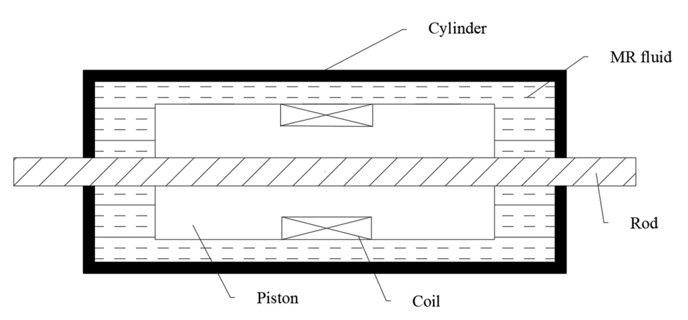
2. Mathematical Model of MR Damper

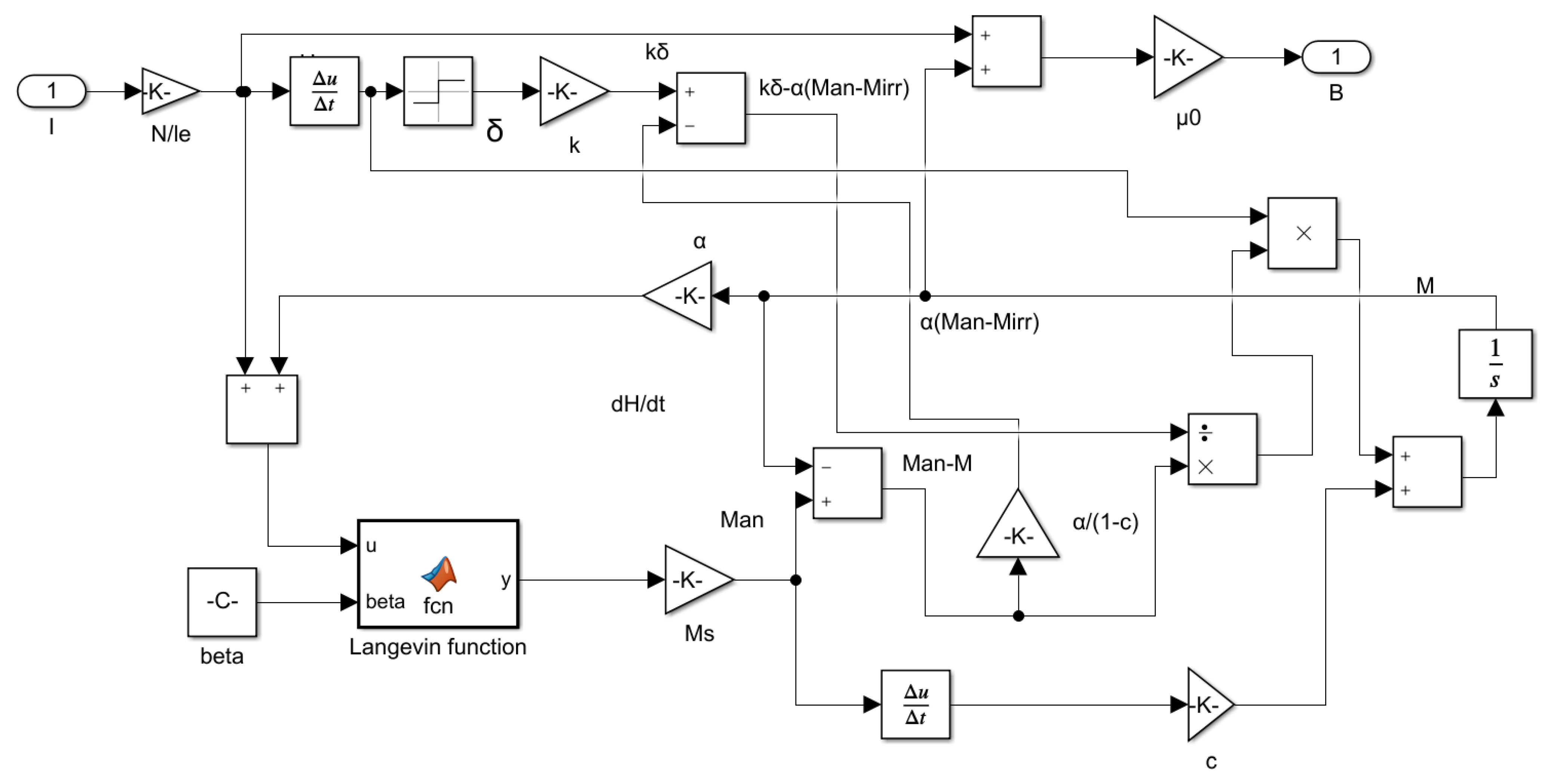
2.1. Jiles–Atherton Hysteresis Model
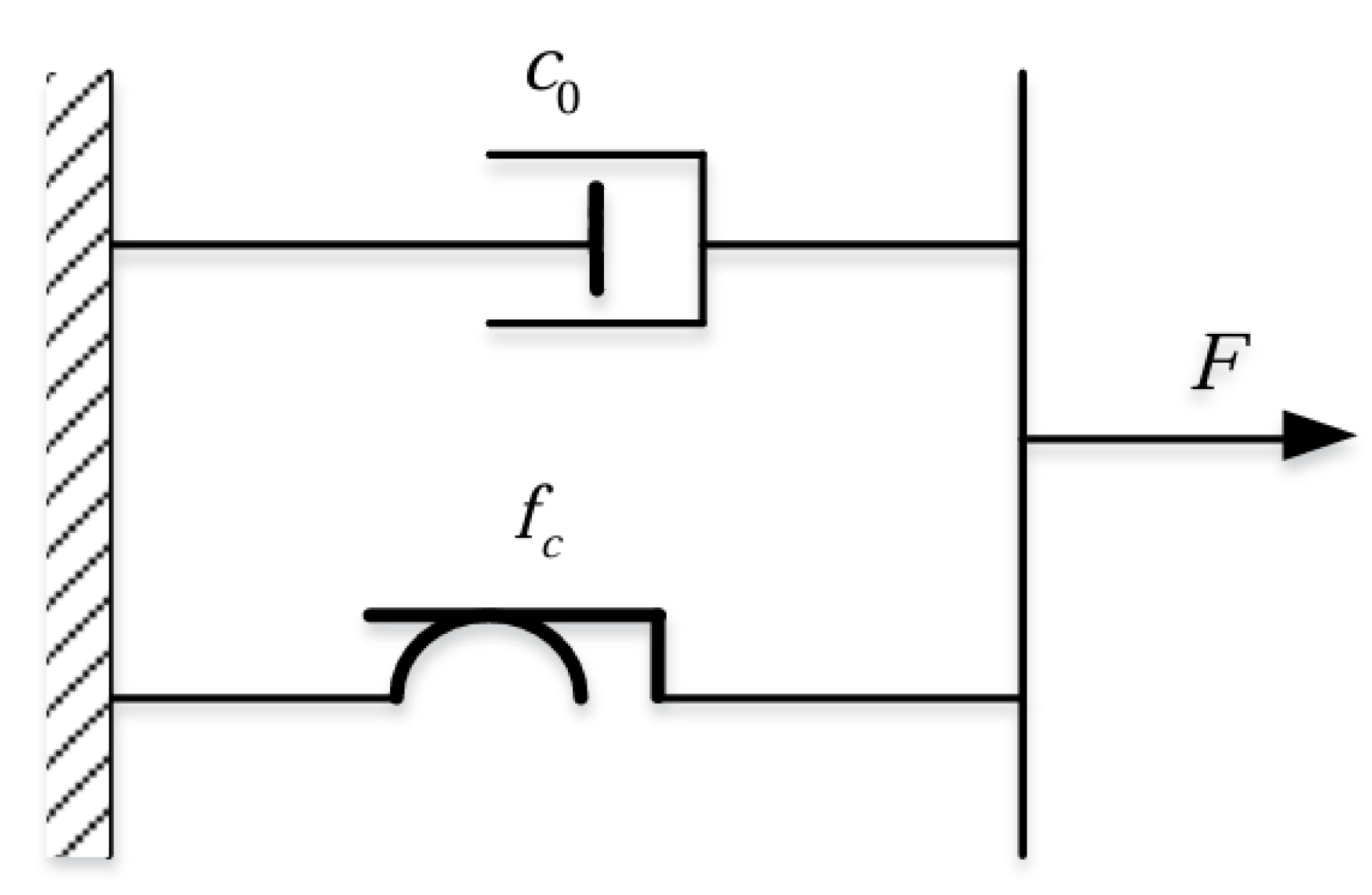
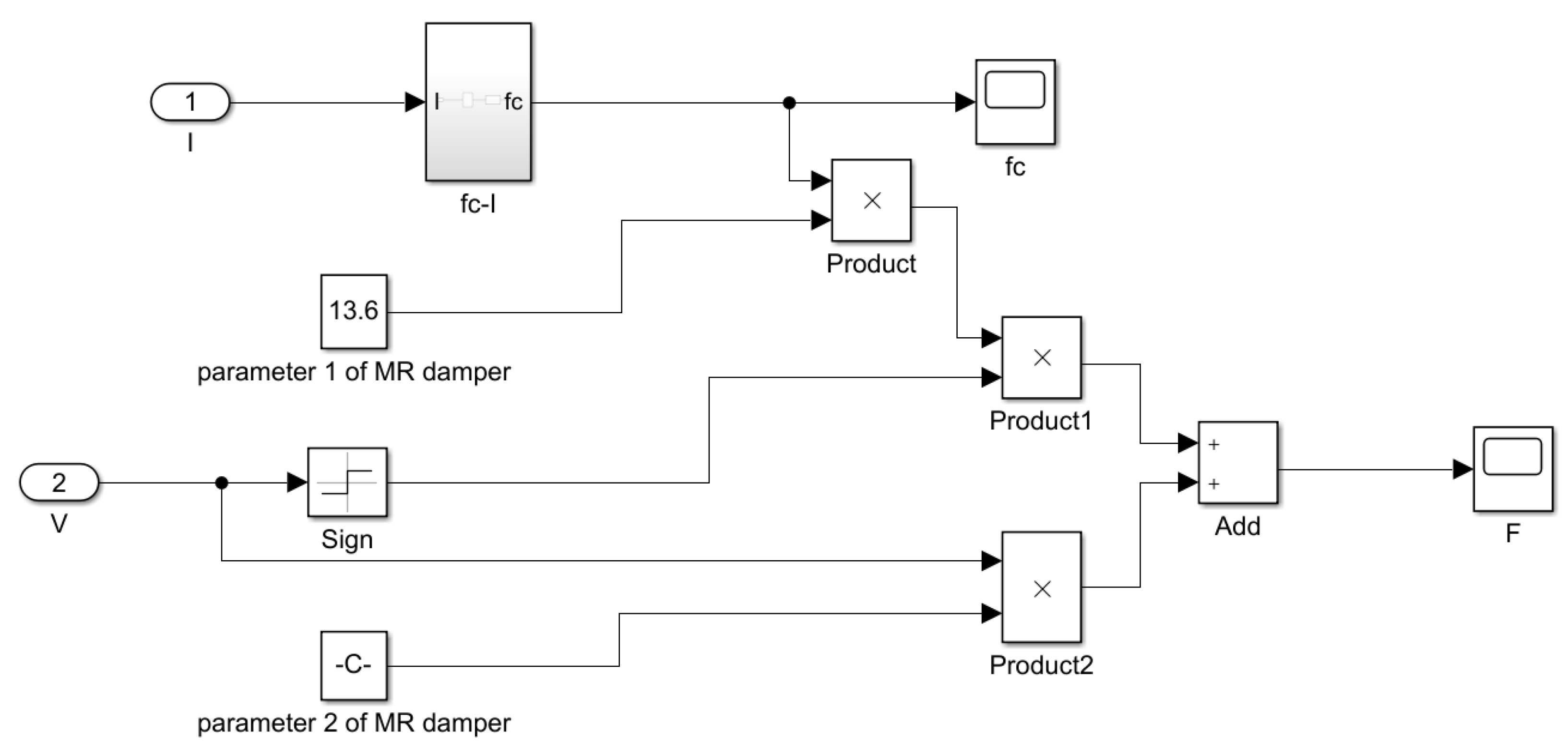
MR dampers have a variety of operating modes and structures, and the most common structure at present is the shear valve single-cylinder double-outlet rod form, as shown in Figure 1, which is mainly composed of MR fluid, a piston rod, sleeve, coil and piston. Under the action of the magnetic field, when the piston moves in a straight line relative to the sleeve, the MR fluid is converted from a Newtonian fluid to a solid-like fluid, which results in the formation of a yield stress. The hysteresis characteristics of the MR fluid will in turn affect the output accuracy of the damper during the change in the magnetic field, so it is extremely critical to model the hysteresis of the MR fluid before performing the mechanical analysis of the MR dampers.
The J-A model splits the actual magnetization M into a reversible magnetization component Mrev and an irreversible magnetization component Mirr [25]:
M = M rev + M irr
Mrev and Mirr can be obtained from the hysteresis-free magnetization Man:
M rev = c ( M an M irr )
where c is the reversible magnetization factor.
The Man is described by a modified Langevin function [26]:
M an = M S coth ( H e β ) β H e
where M S is the saturation magnetization. H e is the effective magnetic field strength, and β is the shape parameter of the hysteresis-free magnetization.
H e can be expressed as:
H e = H + α M
where α is the domain–wall interaction coefficient and H is the magnetic field strength.
μ 0 M d H e = μ 0 M an d H e μ 0 k δ d M i r r d H e d H e
where k is the hysteresis loss parameter, μ 0 is the vacuum permeability, and δ is a parameter indicating the direction of change of the magnetic field; when d H / d t > 0 , (the magnetic field gradually increases with time), δ = 1 ; and when d H / d t < 0 , (the magnetic field gradually decreases with time), δ = 1 .
The derivation of Equation (5) is obtained:
d M i r r d H e = M a n M k δ
Based on the above equations, the differential equation for the J-A model is expressed as:
d M d H = ( M an M ) + c k δ d M a n d H e k δ α ( M a n M )
From electrodynamics, it is clear that
B = μ 0 ( H + M )
The calculated metric for the magnetic field strength in a magnetic circuit is:
H = N I L e
where I is the excitation current, and L e is the effective magnetic circuit length.
According to Equations (8) and (9), the M-H equation in the J-A hysteresis model can be converted to the B-I equation. Considering that the J-A hysteresis model is a time-based differential equation in the actual simulation, the conversion of Equation (7) to differentiation with respect to time t yields
d M d t = ( 1 c ) M an M irr k δ α ( M an M irr ) d H d t + c d M an d t M an = M S coth ( H e β ) β H e

2.2. Bingham Model

In this paper, the Bingham model [27] is adopted as the mathematical model of MR dampers. As shown in Figure 2. the model consists of a Coulomb friction element as well as a linear viscous unit, and the physical meaning of the parameters characterized by the Bingham model is clear and precise and the number of variable parameters is small, which can satisfy most of the engineering requirements and is widely used. Its mathematical expression is [28]
F = f c sgn ( γ ˙ ) + c 0 γ ˙
where F is the output damping force of the model, f c is the static friction force of the friction element and c 0 is the damping coefficient of the damper element. γ ˙ is the shear strain rate.
The MR damper force–displacement relationship can be further derived as [29]:
F = 3 A P L f c h d sgn ( γ ˙ ) + 12 η L A P 2 π D h d 3 γ ˙
where Ap is the effective area of the piston, L is the effective length of the piston; hd is the effective clearance between the piston and the cylinder; and D is the diameter of the piston.
The MRD-SEU-D050 MR damper used in this article is shown in Figure 3. It adopts the MR fluid developed by Professor Xu Zhao Dong’s team, whose expression for the yield stress versus the magnetic induction is [30]
f c = 146960 B 0.5811 V 1.706 ρ 0.2 M s 0.8 + 1083.2 V 287.03
where B is the magnetic induction, V is the volume fraction of ferromagnetic particles in the MR fluid and ρ is the particle diameter of the ferromagnetic particles.
MRD-SEU-D050 MR damper is a three coil MR damper with a maximum piston stroke of 40 mm, which can output a large damping force. The force–displacement curves under different constant currents are shown in Figure 4.
As shown in Figure 5, the J-A model can characterize the B-I relationship, and B is an important parameter in the force–displacement relationship of the MR damper, so the MR damper force–current relationship can be easily obtained by fusing the J-A model with the MR damper model.
According to Equation (10), it can be seen that in the J-A hysteresis model, k, β , α , Ms and c are five key parameters that affect the accuracy of the hysteresis curve. In order to enable the J-A hysteresis model to characterize the hysteresis properties of the MR damper well, it is necessary to identify the five key parameters in the J-A hysteresis model. In this study, an improved PSO is used to identify these five parameters.

3. Particle Swarm Optimization Algorithm

3.1. Classical Particle Swarm Optimization Algorithm

The Particle Swarm Optimization Algorithm (PSO) is a classical intelligent algorithm, but as researchers delve deeper, more intelligent algorithms are being developed. Compared with the Grey Wolf Algorithm, the PSO has a better global search ability, which can be better applied to the multi-peak optimization problem; compared with the Wale Optimization Algorithm, which has the drawbacks of slow computation time and poor interpretability, the PSO can make up for these problems; compared with the Fruit-fly Optimization Algorithm, some improvements to the PSO can avoid neglecting the differences between different individuals while still maintaining high objectivity. Therefore, this paper chooses PSO as the optimization algorithm for parameter identification.
In PSO, the fitness value of each particle is calculated iteratively, tracking the individual extremes and the population extremes to update its position and velocity until an optimal solution is obtained [31].
The formula for updating the velocity and position of particle i in the nd dimension j is
υ i j ( d + 1 ) = ω υ i j ( d ) + c 1 r 1 p i j ( d ) x i j ( d ) + c 2 r 2 p g j ( d ) x i j ( d ) x i j ( d + 1 ) = x i j ( d ) + υ i j ( d + 1 ) 1 i n 1 j D
where d is the current iteration number, c 1 , c 2 are acceleration factors, r 1 , r 2 are uniform random numbers in the range [0, 1] used to increase the randomness of the particles while flying, n is the number of particles and d is the decision dimension, and ω is inertia factor. υ i j ( d ) denotes the j th dimensional component of the velocity vector of the particle i flight at the d th iteration; x i j ( d ) denotes the j th dimensional component of the velocity vector of the flight of particle i at the d th iteration; p i j ( d ) denotes the historical optimal solution searched by particle i up to the d th iteration; and p g j ( d ) is the global optimal solution searched by the whole particle swarm.
In this study, the root-mean-square error of the measured and calculated magnetic induction is used as the fitness function of the improved PSO, so that the parameter identification problem is converted into a minimum value optimization problem with the fitness function
F _ obj = i = 1 n ( B exp B s i m ) 2 N
where B exp is the experimental value of magnetic induction; B s i m is the calculated value of magnetic induction; and N is the amount of experimental data.
Classical particle swarm searches for the global optimum by following the current optimal solution; the rules of this algorithm are simpler, and it is widely used for its easier implementation, high accuracy, fast convergence, etc. However, the PSO also leads to the problem that it is easy to lose the diversity of the particles and fall into the local optimal solution due to the advantage of the fast convergence speed. Therefore, in order to make the identified parameters more accurate, the PSO needs to be improved.

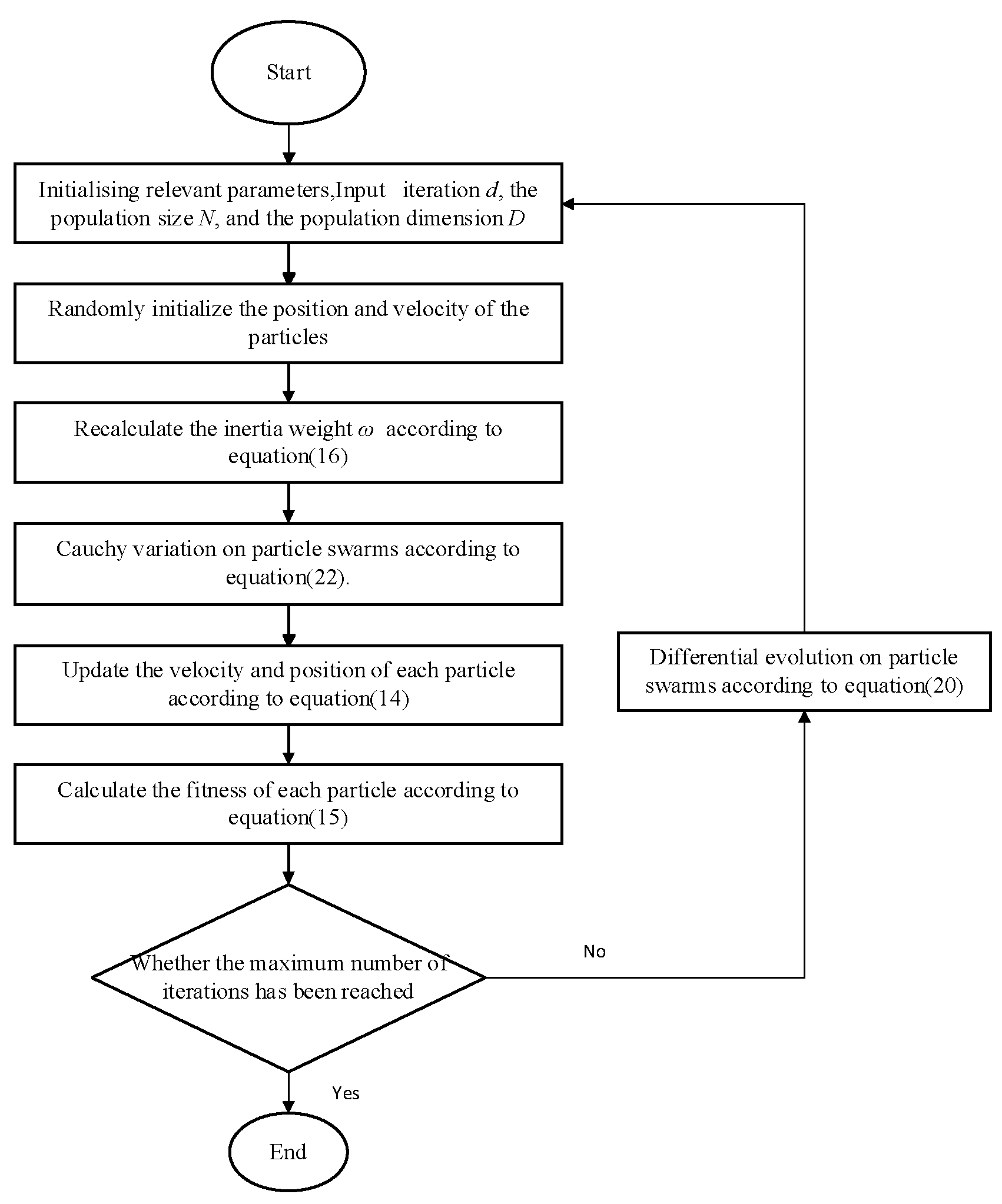
3.2. Improved Particle Swarm Optimization Algorithm

(1)
Weight Adaptation
When the inertia weights are large, the algorithm has a strong global search ability and can search a large area, and when the inertia weights are small, the algorithm has a strong local optimization ability and can search finely around the optimal solution. Therefore, in the last few steps of optimization, in order to improve the accuracy, the inertia weight of the PSO should be gradually reduced. In this paper, a linear decreasing weight method is chosen [32], and its mathematical expression is entered as shown in the following equation:
ω = ω max ω max ω min × d d max
In this paper, ω max is taken as 0.8 and ω min is taken as 0.2, and at each iteration ω is recalculated.
(2)
Differential Evolution
As the number of iterations increases, the population diversity decreases and the particle swarm tends to fall into local optimal solutions. Differential evolution is able to maintain population diversity during iterative search, so incorporating differential evolution improves the global search ability of the particle swarm. Differential evolution is improved on the basis of genetic algorithm [33], and its core parts are all variation, crossover and selection operators; in this paper, the specific definitions of variation, crossover and selection operators of differential evolution are as follows.
(a)
Population Initialization
During the initialization phase, it is necessary to randomly form M individuals with constraint requirements in an n-dimensional space. The specific implementation measures are
q i j ( 0 ) = randl i j ( 0 , 1 ) ( q i j U q i j L ) + q i j L ( 1 )
q i j U , q i j L represent the upper and lower bounds of the j th chromosome, respectively; randl i j ( 0 , 1 ) is a random number in the range [0, 1].
(b)
Mutation
The more common differencing strategy is to select two different individuals among the parent individuals to perform a vector difference operation to generate a difference vector, and then select another individual to be summed with the difference vector to generate a new variant individual. The mathematical description is:
h i j ( d + 1 ) = q p 1 j ( d ) + F ( q p 2 j ( d ) q p 3 j ( d ) )
where h i j ( d + 1 ) denotes the i th individual in the d + 1st generation of the mutant population, q j ( d ) represents the parent individual, p1 p2, p3 are three mutually exclusive random numbers and F is the scaling factor.
(c)
Crossover
The purpose of the crossover operation is to randomly select an individual. Specifically, it is to select the child variant vector for each component according to a certain probability to generate a test individual, and the specific crossover operation formula is
u i j ( d + 1 ) = h i j ( d + 1 ) if   r a n d ( 0 , 1 ) C R x i j ( d ) o t h e r w i s e
where CR is the crossover probability, which is used to control the selection of the variant vector values and the original vector values.
(d)
Selection
The selection operand selects individuals to enter the next generation of the population based on the magnitude of the fitness value.
x i j ( d + 1 ) = u i j ( d + 1 ) if   f ( u i j ( d + 1 ) ) f ( x i j ( d ) ) x i j ( d )  
(3)
Cauchy Variation
The particle aggregation in the late iteration of the algorithm is obvious and shows strong convergence, and it is easy to fall into the premature convergence state, so after the algorithm falls into premature convergence, the Cauchy variation operation [34] is introduced to maintain the diversity of the particle population, so that the algorithm has the ability to jump out of the local optimum.
The longer distribution at both ends of the Cauchy density function not only gives individuals a higher probability of jumping out of the local optimum, but also the variant produces greater variability between the offspring and the parents, and thus the Cauchy variant is more perturbing. In this paper, the one-dimensional Cauchy density function is used, and its mathematical expression is
f ( x ) = 1 π 1 x 2 + 1 < x <
The new positional solution generated using the Cauchy variation is
x i j ( d + 1 ) = x i j ( d ) + x i j ( d ) c a u c h y ( 0 , 1 )
where c a u c h y ( 0 , 1 ) is the standard Cauchy distribution function and denotes the multiplicative implication. x i j ( d ) is the global optimal solution of the d-th iteration of particle swarm optimization.
The specific flow chart is as Figure 6.

4. Numerical Analysis

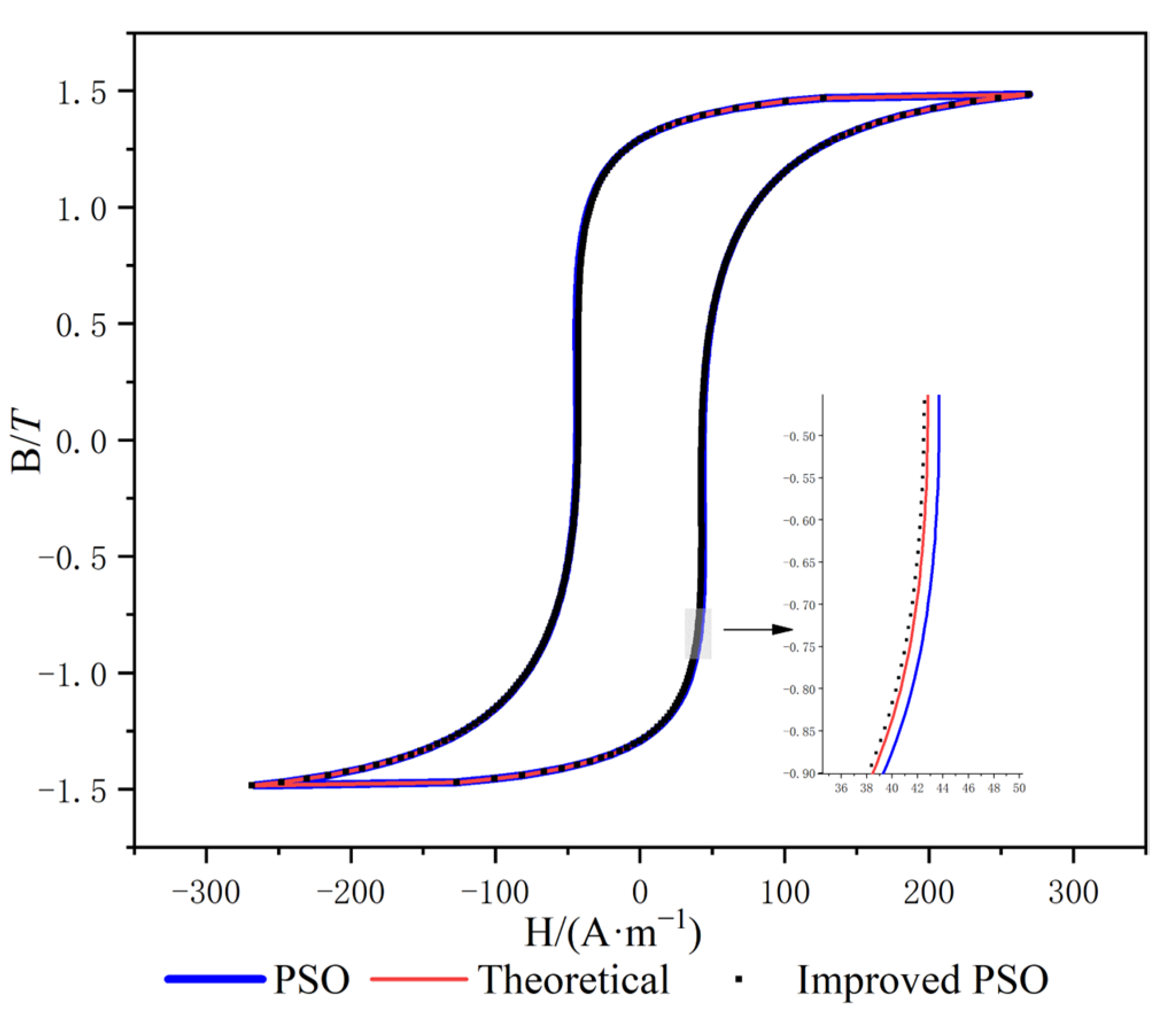
4.1. Algorithm Verification

In order to verify the feasibility of the algorithm, the PSO was initialized, the population size was set to 30, the maximum number of iterations was 150, the search space for each of the five model parameters was set to a region within ±100% of its true value, and for the ω, a linear decrease was taken between 0.8 and 0.2 during the iterations and c1 = c2 = 2 was taken.
In order to verify the effectiveness of the proposed improved particle swarm optimization algorithm in the parameter identification of the J-A hysteresis model, a J-A hysteresis model with known parameters is used as a fitting object according to the parameters in the literature [35]. Based on this B-H curve, the improved particle swarm optimization algorithm is used to identify the parameters of the B-H curve of this J-A hysteresis model, and the corresponding B-H curve as well as the parameter error are calculated. The results of parameter identification are shown in Table 1. The errors of the parameter identification results are shown in Table 2. The B-H curves fitted by the two algorithms are shown in Figure 7, and the algorithm adaptation curves are shown in Figure 8.
According to the results of parameter identification, of the two algorithms at the end of 150 iterations, the improved PSO algorithm that identified the parameter values with the theoretical parameter error is smaller and more accurate, and the fitted B-H curves are more overlapping and more effective.
According to Figure 8, it can be seen that when the algorithm enters the local optimal solution at the beginning of the iteration, the improved particle swarm preferentially jumps out of the local optimal solution, and the objective function converges towards the minimum value, and in the iteration of up to 78 generations, the objective function converges to 0.07, whereas the classical PSO, although it has been fluctuating, cannot achieve the convergence, and the value of fitness is still maintained at 0.422 after the completion of 150 iterations. It is difficult to go further to obtain more accurate results.
According to Table 2, the accuracy of the PSO and the improved PSO for the identification of key parameters in the J-A model can be compared more intuitively. The results obtained by using the improved PSO are more accurate, and the overall relative error of the identification results is smaller; the largest relative error arises from the β, which is only 5.8%. Compared with the PSO, the relative error is reduced by 40.2%.

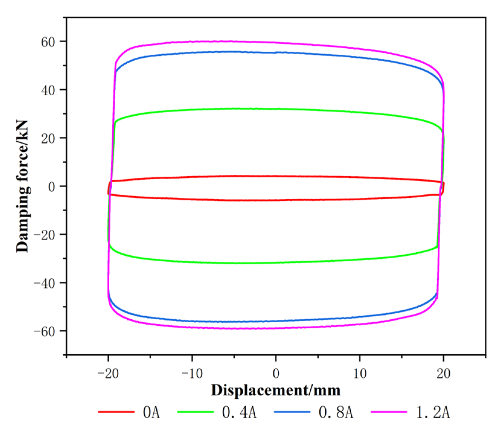
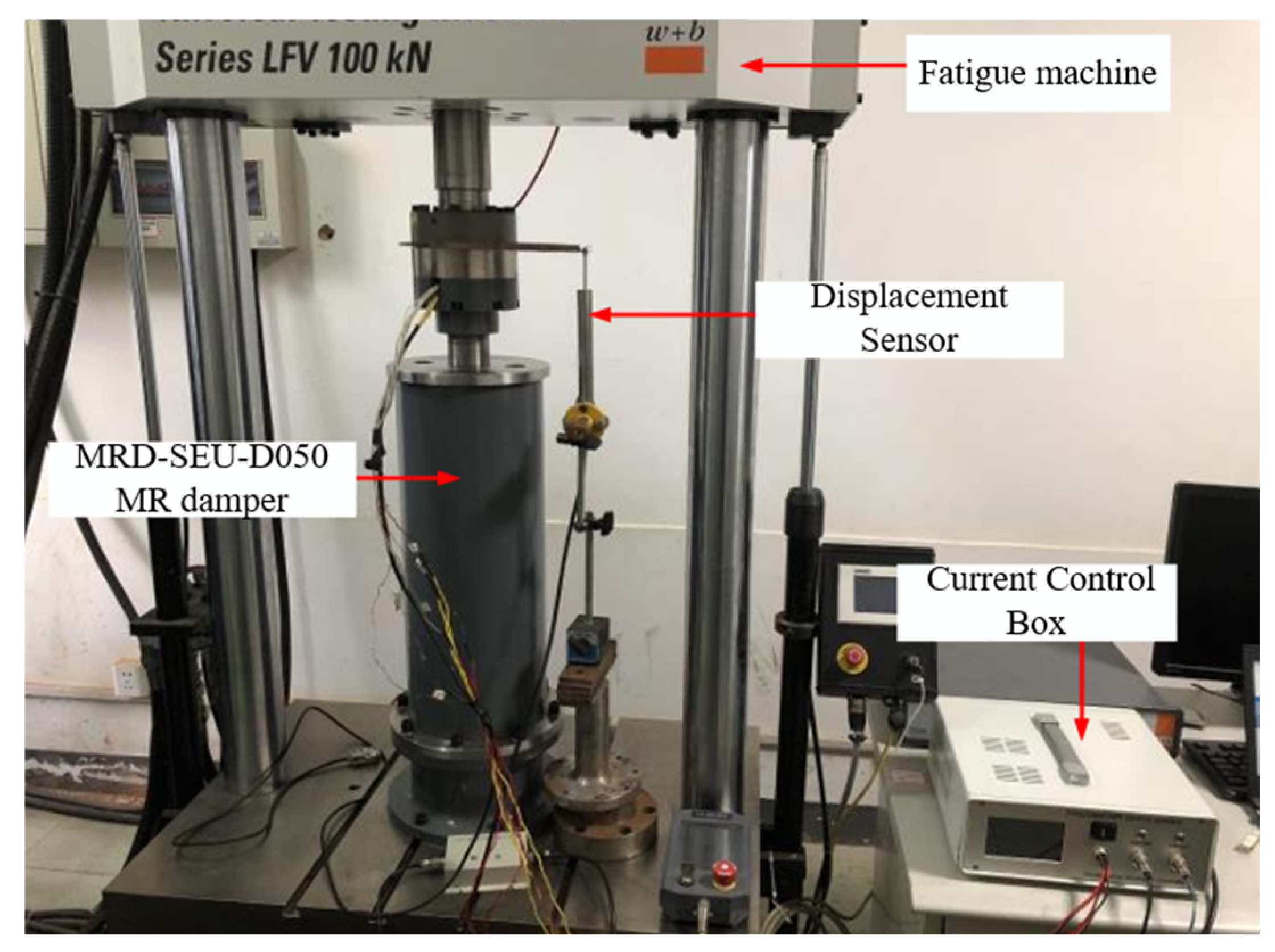
4.2. Experimental Comparison

The above simulation verifies the accuracy of the improved PSO in identifying the parameters of the J-A model. In order to verify its ability to improve the accuracy of the output damping force of the MR dampers, the simulation of the Bingham mechanical model of the MR damper and the J-A hysteresis model are established in Simulink, the specific block diagram of the Bingham mechanical model is shown in Figure 9 and that of the J-A hysteresis model is shown in Figure 10. In Figure 9, “in1” module is the current input module. “in2” module is the velocity input module. Since this model is a velocity-dependent shape model, it is necessary to derive the displacement to obtain the velocity under the relative time. The “parameter 1 of MR damper” module and “parameter 2 of MR damper” module are calculated from the MR damper’s own parameters, which are related to the magnetorheological damper. The subsystem fc-i incorporates the J-A model and is derived from Equation (13). In Figure 10, the “out” module is a magnetic induction output module. The “function” module is used in simulink to express the Langevin function. The J-A hysteresis model is combined into the Bingham mechanical model. For the key parameters in the J-A hysteresis model, the values identified by classical particle swarm and improved particle swarm are used, respectively, and the results simulated by the two algorithms are compared and analyzed with the experimental values and the theoretical values without considering the hysteresis characteristics. In order to accurately measure and more accurately test the experimental value of the output damping force of the magnetorheological damper, this paper adopts the MTS electro-hydraulic servo material performance test fatigue machine as the signal generating experiment, and adopts the LVDT displacement meter to monitor the change in the displacement and to achieve the purpose of variable output current through the intelligent control box. The experimental system is shown in Figure 11. The specific parameters of the MR fluid in the MRD-SEU-D050 magnetorheological vibration damping device used in this test are shown in Table 3. The control current changed with the change of displacement, and its correspondence is shown in Table 4. The fatigue machine was used to apply displacement signals to the MR dampers at different working conditions for the performance test, respectively, and the control current changed with the change in displacement, and its correspondence is shown in Table 4. The damping force–displacement curves generated under the different working conditions are shown in Figure 12.
According to Figure 12, it can be seen that when the frequencies of the displacement excitation signal are 0.05 Hz, 0.1 Hz and 0.2 Hz, respectively, the curves fitted using the model proposed in this paper have a large error with the experimental curves. This is because, when the frequency of the displacement excitation signal is low, the control current changes slowly, the magnetic field generated by the excitation coil changes slowly, the change in the magnetization state of the ferromagnetic particles in the MR fluid can keep up with the change of the applied magnetic field, and the hysteresis characteristics have a small effect on the accuracy of the output damping force of the magnetorheological damper. In order to verify the effect of response frequency on the hysteresis characteristics, this paper resets the frequency of the excitation signal, and the fatigue machine generates a sine wave with a frequency of 1 Hz as the excitation signal, and the force–displacement curve at 1 Hz is shown in Figure 13. It was found that the force–displacement curves at 1 Hz were similar to those at a constant current. This is because the instantaneous response of the magnetic induction is difficult to capture when the displacement excitation signal is accelerated by the current change corresponding to high frequency, so the damping force will be similar to that in the case of constant current. Therefore, this paper does not consider the effect of the response frequency of the excitation signal on the hysteresis characteristics, so the test parameters can be reset, and a comparative analysis of the test carried out under 0.5 Hz operating conditions. The damping force–displacement curves generated at 0.5 Hz working condition are shown in Figure 14.

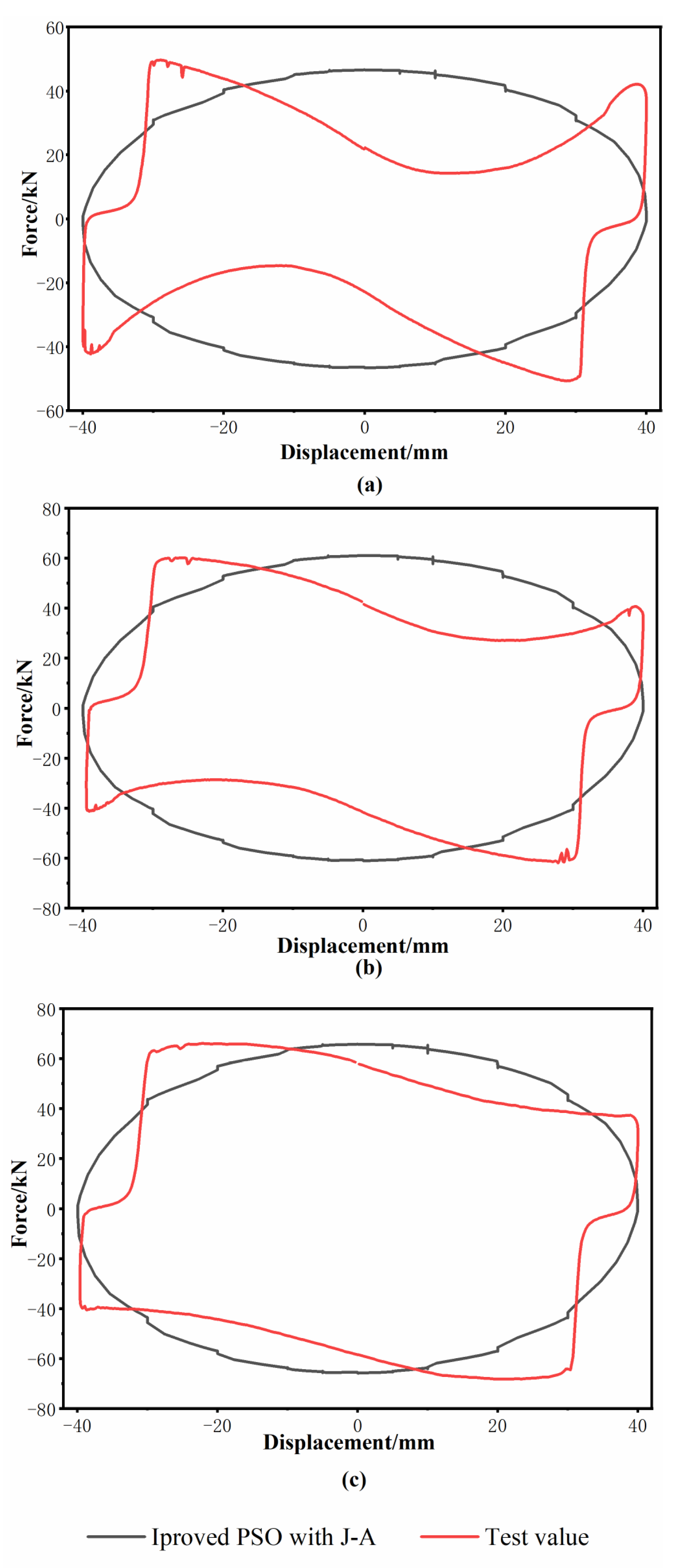
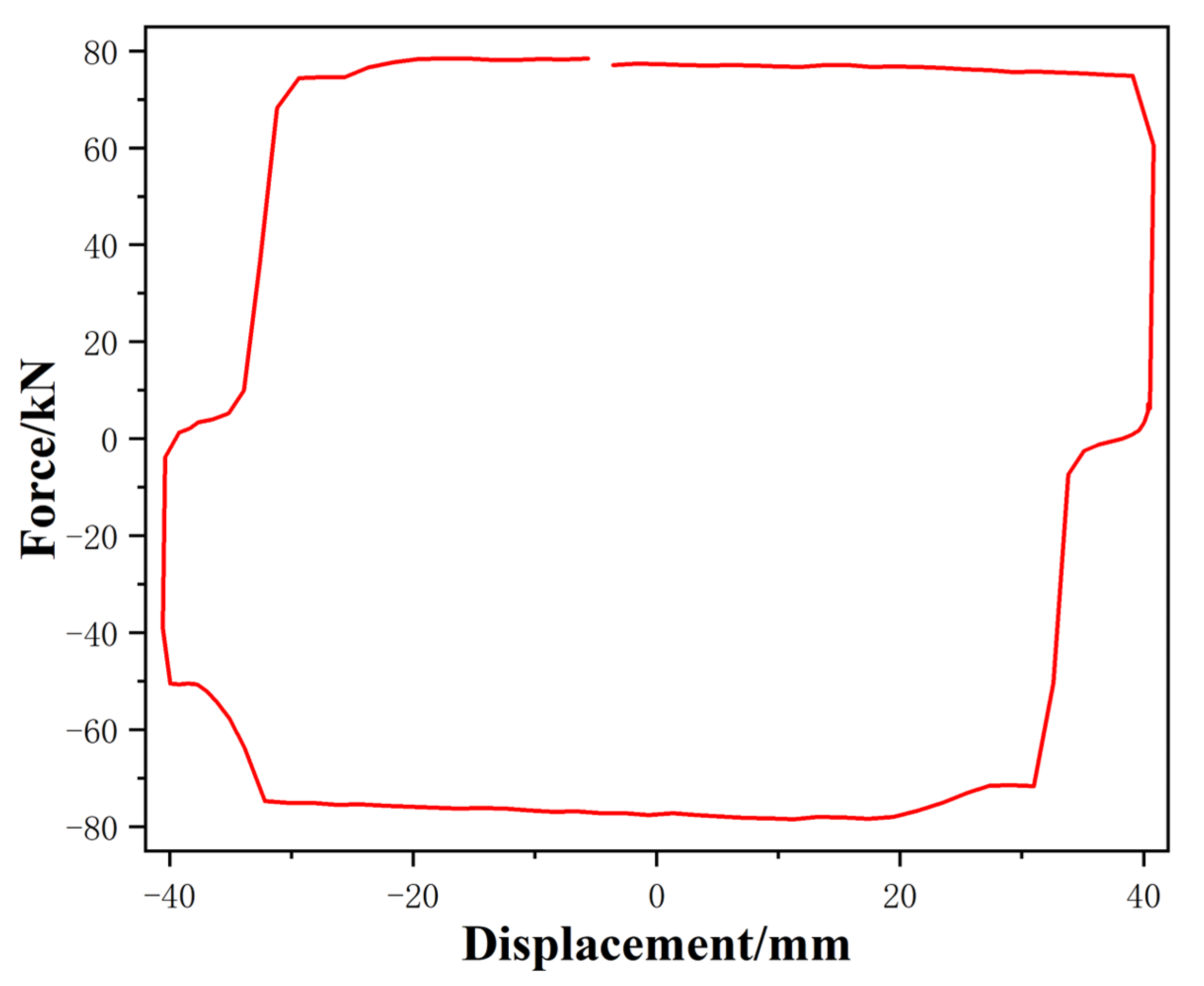
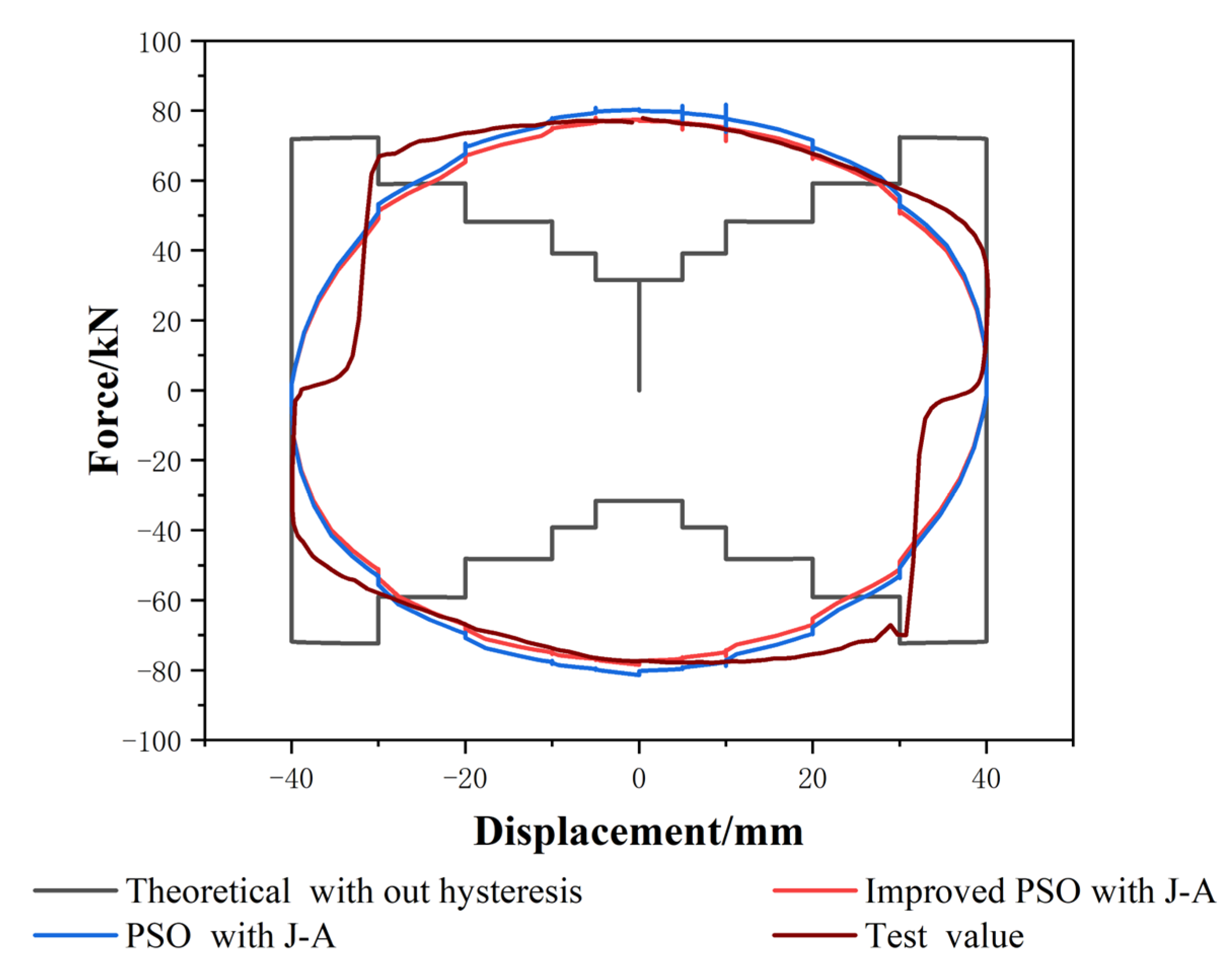
4.3. Results and Discussions

As can be seen from Figure 12, we can find that when the displacement of the damper piston reaches the maximum, there will be an output damping force of 0. This is because when the displacement of the damper reaches the maximum—that is, the piston rod extends the longest part, which means the piston rod needs to reverse the movement—at this time, the piston rod compresses the air first, and when the air is compressed all the way, the damping force will be gradually increased, which explains the displacement of 30–40 mm as well as −40–30 mm. The output damping force is 0, and when the absolute value of the displacement is less than 30 mm, the damping force appears to be jumping. This situation occurs due to the structural design of the MR damper, so that the experimental and simulated values have a large error when the absolute value of the displacement is between 30 mm and 40 mm, and its reference value is small.
As can also be seen from Figure 14, it can be seen that the segmentation of the calculated value without considering the hysteresis characteristic is obvious, and its size is only affected by the control current, and when the displacement becomes bigger and bigger, its error with the test value will also become bigger and bigger. After combining the J-A hysteresis model into the Bingham mechanical model, it can be seen that the output damping force curve is closer to the test value curve. When the absolute value of the piston rod displacement is between 0 mm and 20 mm, comparing the output damping force curves of the two algorithms, the maximum error of the simulation curve and the test curve obtained by using the PSO is 4.68 kN, and the average error is 2.53 kN; the maximum error of the simulation curve and the test curve obtained by using the improved PSO is 2.59 kN, and the average error is 1.46 kN; the maximum error is reduced by 44%, and the average error is reduced by 42%, which shows that when the accuracy of the J-A model is higher, the error between the output damping force and the test value is smaller.
The J-A hysteresis model is combined with the Bingham mechanical model, and the improved PSO is used to identify the parameters of the J-A model. The output damping force and the error of the experimental value have been significantly reduced, and are within a reasonable range, but have not yet reached the optimum, the reasons for which are analyzed as follows: (1) the rheological properties of the MR fluid are easily affected by the temperature and its own settlement characteristics, When the external environment changes, the yield shear stress will also change; (2) the hysteresis characteristics of the MR fluid are not the only reason affecting the hysteresis property of the magnetorheological damper; the magnetic field generated by the excitation coil of the damper itself after energization and the real-time control current will also have hysteresis, which will have an impact on the accuracy of the output damping force of the MR damper.

5. Conclusions

In this study, an improved J-A model was proposed to consider the magnetic hysteresis properties of MR dampers, in which a weighted adaptive PSO was adopted to identify the key parameters. The effectiveness of the proposed J-A model was verified by comparisons with performance test data under different working conditions. The following conclusions can be obtained:
(1)
The improved adaptive PSO which introduces differential evolution algorithm and Cauchy variation strategy on the basis of particle swarm effectively solves the problem that classical PSO falls easily into the local optimal solution; additionally, it solves the problem of the slow convergence of classical PSO, and improves the accuracy of identification.
(2)
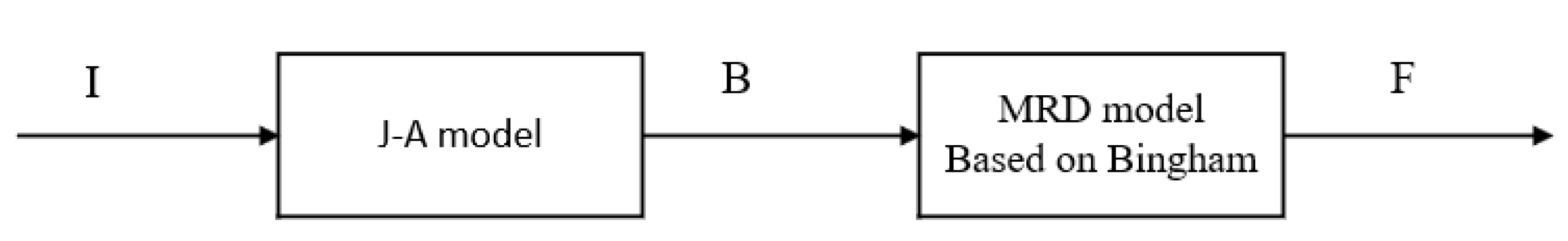
The improved J-A model using the PSO can accurately describe the non-linear relationship between the magnetic induction and the current inside the MR damper, and can accurately predict the output force of MR dampers with magnetic hysteresis properties, providing a basis for the numerical analysis and practical engineering applications of MR dampers.
(3)
In this paper, the effect of hysteresis characteristics on the output damping force is most obvious at 0.5 Hz; however, when the displacement signal response is in the low-frequency band or high-frequency band greater than 1 Hz, there is a large gap between the simulation results and the experimental values, and this paper ignores the effect of the response frequency on the hysteresis characteristics, and at the same time hysteresis characteristics are not only reflected in the change of the magnetic field strength generated by the excitation coil, but also in the internal magnetic circuit of the MR damper. Hysteresis also needs to be modeled and analyzed, which is also the focus of subsequent research.

Author Contributions

Conceptualization, Y.-Q.G. and M.L.; methodology, Y.-Q.G.; software, M.L. and Y.Y.; validation, Y.-Q.G., Z.-D.X. and M.L.; formal analysis, Y.-Q.G., Y.Y. and M.L.; investigation, M.L. and W.-H.X.; resources, Y.-Q.G. and Z.-D.X.; data curation, M.L. and W.-H.X.; writing—original draft preparation, Y.-Q.G. and M.L.; writing—review and editing, Y.-Q.G. and M.L.; visualization, Y.-Q.G. and M.L.; supervision, Y.-Q.G.; project administration, Y.-Q.G.; funding acquisition, Y.-Q.G. All authors have read and agreed to the published version of the manuscript.

Funding

This work was supported by the National Natural Science Foundation of China under grant 52278505.

Institutional Review Board Statement

Not applicable.

Informed Consent Statement

Not applicable.

Data Availability Statement

Data are contained within the article.

Conflicts of Interest

The authors declare no conflicts of interest.

References

  1. Du, X.X.; Zhang, Y.H.; Li, J.H.; Liao, C.R. Unsteady and hysteretic behavior of a magnetorheological fluid damper: Modeling, modification, and experimental verification. J. Intell. Mater. Syst. Struct. 2023, 34, 551–568. [Google Scholar] [CrossRef]
  2. Zhu, J.T.; Xu, Z.D.; Guo, Y.Q. Magnetoviscoelasticity parametric model of an MR elastomer vibration mitigation device. Smart Mater. Struct. 2012, 21, 075034. [Google Scholar] [CrossRef]
  3. Abdalaziz, M.; Sedaghati, R.; Vatandoost, H. Development of a new dynamic hysteresis model for magnetorheological dampers with annular-radial gaps considering fluid inertia and compressibility. J. Sound Vib. 2023, 561, 117826. [Google Scholar] [CrossRef]
  4. Wang, B.; Wang, W.J.; Li, Z.C. Sliding Mode Active Disturbance Rejection Control for Magnetorheological Impact Buffer System. Front. Mater. 2021, 8, 682215. [Google Scholar] [CrossRef]
  5. Aloisio, A.; Boggian, F.; Tomasi, R.; Zeng, K.N. Reliability-Based Assessment of LTF and CLT Shear Walls under In-Plane Seismic Loading Using a Modified Bouc-Wen Hysteresis Model. ASCE-ASME J. Risk Uncertain. Eng. Syst. Part A Civ. Eng. 2021, 7, 04021065. [Google Scholar] [CrossRef]
  6. Ahamed Rashid, M.M.; Ferdaus, M.M.; Yusuf, H.B.R. Modelling and performance evaluation of energy harvesting linear magnetorheological (MR) damper. J. Low Freq. Noise Vib. Act. Control 2017, 36, 177–192. [Google Scholar] [CrossRef]
  7. Yang, Y.; Xu, Z.D.; Guo, Y.Q. Performance tests and microstructure-based sigmoid model for a three-coil magnetorheological damper. Struct. Control. Health Monit. 2021, 28, e2819. [Google Scholar] [CrossRef]
  8. Song, G.; Zhao, J.Q.; Zhou, X.Q.; de Abreu-García, J.A. Tracking control of a piezoceramic actuator with hysteresis compensation using inverse Preisach model. IEEE-ASME Trans. Mechatron. 2005, 10, 198–209. [Google Scholar] [CrossRef]
  9. Lacroix, L.M.; Gieraltowski, J. Magnetic hyperthermia in single-domain monodisperse FeCo nanoparticles: Evidences for Stoner-Wohlfarth behavior and large losses. J. Appl. Phys. 2009, 105, 023911. [Google Scholar] [CrossRef]
  10. Tannous, C.; Gieraltowski, J. The Stoner-Wohlfarth model of ferromagnetism. Eur. J. Phys. 2009, 30, 227. [Google Scholar] [CrossRef]
  11. Sadowski, N.; Sadowski, N.; Batistela, N.J.; Bastos, J.P.A.; Lajoie-Mazenc, M. An inverse Jiles-Atherton model to take into account hysteresis in time-stepping finite-element calculations. IEEE Trans. Magn. 2002, 38, 797–800. [Google Scholar] [CrossRef]
  12. Li, Y.; Zhu, L.H.; Zhu, J.G. Core Loss Calculation Based on Finite-Element Method with Jiles-Atherton Dynamic Hysteresis Model. IEEE Trans. Magn. 2018, 54, 1300105. [Google Scholar] [CrossRef]
  13. Raghunathan, A.; Raghunathan, A.; Melikhov, Y.; Snyder, J.E.; Jiles, D.C. Generalized form of anhysteretic magnetization function for Jiles-Atherton theory of hysteresis. Appl. Phys. Lett. 2009, 95, 172510. [Google Scholar] [CrossRef]
  14. Duan, J.D.; Lei, Y.; Li, H. Research on Ferromagnetic Components J-A Model—A Review. In Proceedings of the 2018 International Conference on Power System Technology (POWERCON), Guangzhou, China, 6–9 November 2018; pp. 3288–3294. [Google Scholar]
  15. Zhu, R.; Fei, Q.G.; Jiang, D.; Marchesiello, S.; Anastasio, D. Identification of Nonlinear Stiffness and Damping Parameters Using a Hybrid Approach. AIAA J. 2021, 59, 4686–4695. [Google Scholar] [CrossRef]
  16. Leite, J.V.; Avila, S.L.; Batistela, N.J.; Carpes, W.P. Real coded genetic algorithm for Jiles-Atherton model parameters identification. IEEE Trans. Magn. 2004, 40, 888–891. [Google Scholar] [CrossRef]
  17. Trapanese, M. Identification of parameters of the Jiles-Atherton model by neural networks. J. Appl. Phys. 2011, 109, 07D355. [Google Scholar] [CrossRef]
  18. Ding, F.J.; Jia, X.D.; Hong, T.J.; Xu, Y.L. Flow Stress Prediction Model of 6061 Aluminum Alloy Sheet Based on GA-BP and PSO-BP Neural Networks. Rare Met. Mater. Eng. 2020, 49, 1840–1853. [Google Scholar]
  19. Chen, Z.G.; Yu, Y.; Wang, Y.X. Parameter Identification of Jiles-Atherton Model Based on Levy Whale Optimization Algorithm. IEEE Access 2022, 10, 66711–66721. [Google Scholar] [CrossRef]
  20. Wang, A.M.; Meng, J.J.; Xu, R.X.; Li, D.C. Parameter Identification and Linear Model of Giant Magnetostrictive Vibrator. Discret. Dyn. Nat. Soc. 2021, 2021, 6676911. [Google Scholar] [CrossRef]
  21. Ni, C.; Wang, D.Y.; Vinson, R.; Holmes, M. Automatic inspection machine for maize kernels based on deep convolutional neural networks. Biosyst. Eng. 2019, 178, 131–144. [Google Scholar] [CrossRef]
  22. Wu, Z.Q.; Hu, X.Y.; Ma, B.Y.; Hou, C.L. SOC estimation of lithium batteries based on RFF and GWO-PF. J. Metrol. 2022, 43, 8. [Google Scholar]
  23. Aggarwal, A.; Dimri, P.; Agarwal, A.; Bhatt, A. Self adaptive fruit fly algorithm for multiple workflow scheduling in cloud computing environment. Kybernetes 2020. ahead-of-print. [Google Scholar] [CrossRef]
  24. Deng, L.; Liu, S. A multi-strategy improved slime mould algorithm for global optimization and engineering design problems. Comput. Methods Appl. Mech. Eng. 2023, 404, 115764. [Google Scholar] [CrossRef]
  25. Wilson, P.R.; Ross, J.N.; Broen, A.D. Optimizing the Jiles-Atherton model of hysteresis by a genetic algorithm. IEEE Trans. Magn. 2001, 37, 989–993. [Google Scholar] [CrossRef]
  26. Guralnik, G.; Pehlevan, C. Effective potential for complex Langevin equations. Nucl. Phys. B 2009, 822, 349–366. [Google Scholar] [CrossRef]
  27. Xu, Z.D.; Shen, Y.P.; Guo, Y.Q. Semi-active control of structures incorporated with magnetorheological dampers using neural networks. Smart Mater. Struct. 2003, 12, 80–87. [Google Scholar] [CrossRef]
  28. Li, W.H.; Du, H. Design and experimental evaluation of a magnetorheological brake. Int. J. Adv. Manuf. Technol. 2003, 21, 508–515. [Google Scholar] [CrossRef]
  29. Yang, Y.; Xu, Z.D.; Xu, Y.W.; Guo, Y.Q. Analysis on influence of the magnetorheological fluid microstructure on the mechanical properties of magnetorheological dampers. Smart Mater. Struct. 2020, 29, 115025. [Google Scholar] [CrossRef]
  30. Sun, C.L.; Xu, Z.D.; Dai, J. Testing and Mechanical Modelling of Hybrid Coated Ferromagnetic Particle-Based Magnetorheological Fluids. J. Southeast Univ. Nat. Sci. Ed. 2019, 49, 328–333. [Google Scholar]
  31. Li, C.H.; Liu, Y.; Zhou, A.M.; Kang, L.S. A fast particle swarm optimization algorithm with cauchy mutation and natural selection strategy. In Advances in Computation and Intelligence, Second International Symposium, ISICA 2007, Wuhan, China, 21–23 September 2007, Proceedings; Kang, L., Liu, Y., Zeng, S., Kang, L., Liu, Y., Zeng, S., Eds.; Springer: Berlin/Heidelberg, Germany, 2007; pp. 334–343. [Google Scholar]
  32. Janakiraman, S.; Priy, M.D. Hybrid grey wolf and improved particle swarm optimization with adaptive intertial weight-based multi-dimensional learning strategy for load balancing in cloud environments. Sustain. Comput. Inform. Syst. 2023, 38, 100875. [Google Scholar] [CrossRef]
  33. Qin, A.K.; Huang, V.L.; Suganthan, P.N. Differential Evolution Algorithm with Strategy Adaptation for Global Numerical Optimization. IEEE Trans. Evol. Comput. 2009, 13, 398–417. [Google Scholar] [CrossRef]
  34. Yang, J.H.; Zhao, X.L.; Mei, J.J.; Wang, S. Total variation and high-order total variation adaptive model for restoring blurred images with Cauchy noise. Comput. Math. Appl. 2019, 77, 1255–1272. [Google Scholar] [CrossRef]
  35. Chwastek, K. Modelling offset minor hysteresis loops with the modified Jiles-Atherton description. J. Phys. D Appl. Physics 2009, 42, 165002. [Google Scholar] [CrossRef]
Figure 1. Schematic structure of the shear valve type single-cylinder double-outlet rod MR damper.
Information 15 00101 g001
Figure 2. Bingham mechanical model.
Information 15 00101 g002
Figure 3. MRD-SEU-D050 MR damper.
Information 15 00101 g003
Figure 4. Force–displacement curves of the MRD-SEU-D050 MR damper at different constant currents.
Information 15 00101 g004
Figure 5. Schematic block diagram of the relationship between the J-A model and the MR damper model.
Information 15 00101 g005
Figure 6. Flow chart of the improved PSO.
Information 15 00101 g006
Figure 7. Comparison of the two algorithms for fitting B-H curves.
Information 15 00101 g007
Figure 8. Comparison of the adaptation values of the two algorithms.
Information 15 00101 g008
Figure 9. Simulation of Bingham mechanical model of MR damper.
Information 15 00101 g009
Figure 10. Simulation of J-A hysteresis model.
Information 15 00101 g010
Figure 11. Experimental system.
Information 15 00101 g011
Figure 12. Comparison of the output damping force–displacement curves of the magnetorheological damper under different working conditions: (a) 0.05 Hz, (b) 0.1 Hz, (c) 0.2 Hz.
Information 15 00101 g012
Figure 13. Output damping force–displacement curves of MR damper at 1 Hz working condition.
Information 15 00101 g013
Figure 14. Comparison of output damping force–displacement curves of MR damper at 0.5 Hz working condition.
Information 15 00101 g014
Table 1. Parameter identification results.
ParameterTheoretical ValuePSOImproved PSO
k (A/m)66.670.9666.51
α (A/m)25.320.0325.32
c (A/m)0.200.250.19
Ms1.3 × 1061.27 × 1061.31 × 106
β 8.43 × 10−57.61 × 10−58.92 × 10⁻⁵
Table 2. Error of parameter identification results.
Algorithmk (A/m) α (A/m)c (A/m)Ms β
Absolute ErrorPSO4.365.270.053 × 1048.2 × 10−6
Improved PSO0.090.020.0110,0004.9 × 10−6
Relative Error (%)PSO6.5420.55252.39.7
Improved PSO0.130.0750.75.8
Table 3. Basic parameters of MR fluid.
Granule   Diameter   r / μ m Cladding Thickness
t / μ m
Volume Fraction
V / ( % )
Zero-Field Viscosity
η 0 / ( Pa s )
1.50.01535~452~2.5
Table 4. Correspondence between control current and displacement signal.
Displacement |x|(mm)≤55 < x ≤ 1010 < x ≤ 2020 < x ≤ 3030 < x ≤ 40>40
Current
(A)
00.20.40.60.81.2
Disclaimer/Publisher’s Note: The statements, opinions and data contained in all publications are solely those of the individual author(s) and contributor(s) and not of MDPI and/or the editor(s). MDPI and/or the editor(s) disclaim responsibility for any injury to people or property resulting from any ideas, methods, instructions or products referred to in the content.

