Abstract
Great advances in stitching high-quality retinal images have been made in recent years. On the other hand, very few studies have been carried out on low-resolution retinal imaging. This work investigates the challenges of low-resolution retinal images obtained by the D-EYE smartphone-based fundus camera. The proposed method uses homography estimation to register and stitch low-quality retinal images into a cohesive mosaic. First, a Siamese neural network extracts features from a pair of images, after which the correlation of their feature maps is computed. This correlation map is fed through four independent CNNs to estimate the homography parameters, each specializing in different corner coordinates. Our model was trained on a synthetic dataset generated from the Microsoft Common Objects in Context (MSCOCO) dataset; this work added an important data augmentation phase to improve the quality of the model. Then, the same is evaluated on the FIRE retina and D-EYE datasets for performance measurement using the Peak Signal-to-Noise Ratio (PSNR) and Structural Similarity Index (SSIM). The obtained results are promising: the average PSNR was 26.14 dB, with an SSIM of 0.96 on the D-EYE dataset. Compared to the method that uses a single neural network for homography calculations, our approach improves the PSNR by 7.96 dB and achieves a 7.86% higher SSIM score.
1. Introduction
While the World Health Organization, as estimated by the 2019 World Sight Report [1], says that 2.2 billion people worldwide suffer from some domain of visual impairment, nearly 1 billion of the cases are avoidable or treatable. In this scenario, early detection and accurate diagnosis of eye pathologies become critical for the prevention of loss of vision and the maintenance of patients’ quality of life. One of the biggest challenges to eye health is the lack of ophthalmologists, especially in remote distanced places and developing countries. This is causing a deficiency in access to timely diagnosis and high-quality management of eye disorders. On the other hand, advances in technology—like the one represented by the empowerment of hand-held mobile phones equipped with the D-EYE device for digital imaging of the retina [2]—open up new opportunities for early diagnosis.
Eye screening by visualizing the retina through fundus imaging offers an opportunity to non-invasively examine the systemic microcirculation in the human retina. Detailed clinical observations of the characteristics of the retinal fundus contribute not only to detecting eye diseases but also to identifying early indicators of a wide range of pathologies, such as diabetes, stroke, hypertension, arteriosclerosis, cardiovascular, neurodegenerative, renal and fatty liver diseases [3].
One challenge that limits the early detection of vision pathologies is the need for more professionals in regions far from large urban centers, especially in developing countries. A limited amount of the literature exists pertaining to the number of optometrists and related ophthalmic personnel. According to a recent study conducted in 2019, which examined the ophthalmology workforce in 198 countries, representing 94% of the global population, it was found that despite the increasing number of practicing ophthalmologists in most countries, there exists an uneven distribution and a significant shortfall in the current and projected number of ophthalmologists [4]. According to the International Agency for the Prevention of Blindness (IAPB), there are critical human resource shortages for allied ophthalmic personnel, especially in sub-Saharan Africa [5].
Considering this gap, methods that can help in the screening process for ocular pathologies can be great allies for ophthalmologists and patients. One viable option for retinal screening is using mobile devices, such as the D-EYE device [6].
Although devices like the D-EYE have been developed as a low-cost tool to capture images of the fundus with just a simple attachment to a smartphone, these still have limitations in image quality. Figure 1 shows some frames of a video obtained with the D-EYE device, and as can be observed, the images contain a perceptible amount of noise and cannot always allow a complete visualization of the optic disk, which is the region of interest for a possible diagnosis, and it is already just a tiny part of the image.
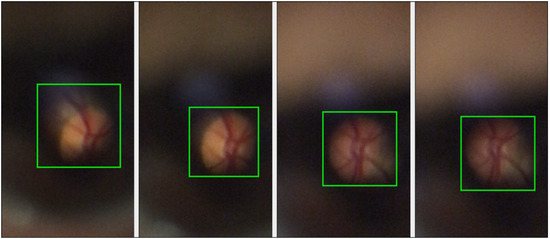
Figure 1.
Different frames of the same video obtained by the D-EYE; the green squares indicate the visible contents of the optic disk and retina.
Among the few studies in the literature related to the problem of low-resolution retinographies, image stitching is the one developed by [7], presenting a comprehensive method that includes the steps of retinal segmentation, identification and matching of reference points, image alignment, and fusion. Variation in the video capture conditions, for example, due to changes in the retinal illumination, impacts the consistency of the results realized with this method. Furthermore, investigating the detection and montage of low-quality retinal images [8], brought out the approach of Super Retina by [9]. This method used semi-supervised deep learning model training techniques for keypoint detectors and descriptors involving the proposed Keypoint Progressive Expansion (KPE) technique, which addresses incompleteness issues arising from the manual labeling of data used in training. Although Super Retina was mostly tested on high-resolution images, it achieved remarkable feature matching and produced well-aligned results. Another technique reviewed by [8] was the stitching of several images suggested by [10], expected to give a complete image with captures obtained from an attached smartphone. This may be a very promising approach for retrieving a complete exposure of the retina, using Uniform Robust Scale-Invariant Feature Transform (UR-SIFT) [11] for feature detection and combining techniques for feature matching and refinement. However, the effectiveness of low-quality images, such as those obtained with D-EYE, may require the application of image pre-processing and image stitching techniques to improve visualization and analysis, both by experts and by automatic methods.
Therefore, this paper aims to address the problem of low-resolution retinal images by employing the image stitching technique to improve the visualization of images captured by the D-EYE. Thus, a method for image stitching between low-resolution retinographies via homography estimation is proposed based on the homography estimation model proposed by [12] with relevant modifications. Thus, we can highlight the following contributions: (1) we proposed a Fundus Blur Filter (FBF) originally designed in this study to mitigate the variations arising from the image capture conditions, which is fundamental to the success of the method; (2) we proposed a modification to the homography estimation network architecture in [12], utilizing four independent semi-siamese convolutional neural networks for more precise coordinate regression, instead of the original single regression.
The rest of this paper is organized as follows. Section 2 presents the proposed method, including the method for generating the synthetic dataset used to train the deep learning model used in homography estimation and the FBF applied to the input images during the model training, originally created for and used in this work, which is essential for the model to work. Section 3 presents the results of the proposed method and discusses the results. Section 4 presents the conclusions and future work.
2. Materials and Method
This section describes the proposed method for image stitching on low-resolution retinal images. First, we describe the dataset used to train the deep learning model. Next, we discuss the different stages of the proposed method, including data augmentation, feature extraction, and homography estimation, as well as the evaluation metrics and experimental setup used to validate the method.
2.1. Synthetic Dataset
Training a neural network for image stitching typically necessitates a large dataset [13,14]. Due to the scarcity of datasets specifically related to stitching low-resolution retinal images, the approach presented by [13] was used as a base for the generation of the synthetic dataset used in this work, modified to suit the needs of this application. For this, 80,000 images from the MS COCO dataset [15] were used.
Each image in the MS COCO dataset is cropped, adjusted to a square format, and resized to 274 × 274 pixels. Subsequently, a new crop is taken from the center of each image, represented in Figure 2A by the white square, which becomes the first input to the neural network. A position—blue square in Figure 2A—for the second crop is marked to ensure overlap with the first. The corners of this position are adjusted to simulate slight variations in the viewing angle, causing deformation relative to the initial marking; the deformed blue square is represented by the orange square in Figure 2B. The pixel distances between the corners of the original second crop position and the deformed marking are recorded as the label for the deep learning model, used in calculating the displacement needed in each corner of the second image to align with the first. The image is then warped so that the corners of the second crop form a square (orange square in Figure 2C), which serves as the second input to the network. The label for the stitching is the union of white and blue square contents in Figure 2B, as can be seen in Figure 2D. Experiments were conducted by adjusting the overlap between images within 50% to 100%. Such adjustments consider the characteristics of images obtained through D-EYE, which are captured from videos, allowing for increased overlap when selecting adjacent frames.

Figure 2.
Synthetic dataset generation steps. (A) Delimitation of the first image pair used to train the network. (B) Small angle variations are applied to the image delimited in (A). (C) Deformed image for using as the second input to the network (D). Label for the stitching, resulting from the union of the contents of the white and orange squares in (B).
2.2. Proposed Method
The proposed method for estimating homography in low-resolution retinal images was inspired by the work of [12], with some adaptations.
A Fundus Blur Filter is applied exclusively during the training phase to deal with variations in the image capture condition, a Siamese convolutional neural network [16,17] for feature extraction, a feature correlation layer, and a regression network to predict the points that will be used to calculate homography using the Direct Linear Transformation (DLT) algorithm [18]. Figure 3 shows the proposed method pipeline.
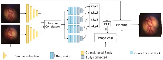
Figure 3.
Proposed method pipeline.
2.2.1. Data Augmentation
Similar approaches for synthetic dataset generation are common in training homography estimation models [12,19]. However, it has disadvantages for predicting homography between image crops obtained under different lighting conditions, as a deep learning model usually performs optimally when it is fed with data closely similar to those samples seen during training [20]. In order to avoid this limitation and achieve generalization, especially with low-resolution images coming from the same retina captured at different moments, a significant innovation was introduced. Thus, we proposed a filter, denominated Fundus Blur Filter (FBF) (Figure 4), consisting of a black image with a white ellipse and a circle surrounding the ellipse, which was applied randomly in terms of position and size around the center of the image. This filter varies the input images’ intensity toward the ellipse, making the model more robust to variations that D-EYE images may contain. Such modification generalizes the model between crops of the same image and between images of the same retina captured at different moments, making the approach adaptable to varying image acquisition conditions.

Figure 4.
Example of Fundus Blur Filter application. (A) Filter’s creation. (B) Input images. (C) Inputs with filters applied. (D) Sample from the D-EYE image dataset.
An improvement was introduced to overcome the limitations in predicting homography between images obtained under different lighting conditions in low-resolution retinal images, such as those faced by [7]. This improvement provides an effective strategy for ensuring the robustness and generalizability of the homography estimation model.
The proposed solution involves applying a blur filter consisting of a black mask containing a white ellipse and a surrounding circle, with random positions and sizes around the center of the image. This filter is then applied to the input images during training, gradually adjusting the intensity towards the ellipse, as shown in Figure 4. To do this, Equation (1) is used, where is the input image at position x, is the filter at position x, is the resulting image at position x, and controls the blending ratio [21].
By gradually adjusting the intensity of the images towards the ellipse, we improve the model’s ability to deal with the nuances in the images captured by the D-EYE device. The FBF allows the model to generalize between clippings of the same image and between images captured at different times with variations in retinal illumination, thus improving the quality and consistency of the stitching process. The implementation details of the FBF are outlined in Algorithm 1, while the parameters used in the experiments conducted in this work are presented in Table 1.
| Algorithm 1. Fundus_Blur_Filter |
|

Table 1.
Parameters of the Fundus Blur Filter.
2.2.2. Feature Extraction
Feature extraction is one of the significant steps in image stitching, which helps match the features between images to estimate the geometric relationship. Therefore, an approach motivated by the work in [12] is used, in which a Siamese convolutional neural network was used for feature extraction along with a feature correlation layer.
In this work, the input images are transformed to grayscale, following most of the practices on training homography estimation models [19,22,23]. The architecture of the network consists of two identical sub-networks with the same weights, each one being composed of four blocks, where each block has a convolutional layer with kernel size and a stride of 1. The number of output filters in the first two layers is 64, and 128 in the last two layers. Batch normalization and max-pooling 2D with a pool size of are applied after each convolutional layer to reduce the data dimension, followed by a ReLU activation function. The sub-networks process the input images in parallel and extract their feature maps, which are then passed to the subsequent Feature Correlation phase. Figure 5 depicts this architecture, where Feature Map contains the features extracted from Input Image 1, and Feature Map contains the features extracted from Input Image 2.
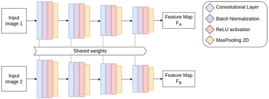
Figure 5.
Feature extraction network architecture.
2.2.3. Feature Correlation
The next step in the network is the feature correlation layer, following the feature extraction phase, where the correspondences between feature maps and extracted from Input Images 1 and 2, are calculated using the proposed method in [12].
Here, L2 normalization is applied to the feature maps and , ; then, correspondences between these two maps are obtained. W, H, and C represent the dimensions of the feature maps, respectively, as well as the width, height, and number of filters (channels). The correspondence at every position in with regard to all positions in is calculated as follows:
where are positions in feature maps, while is a one-dimensional feature vector at position in the feature map . , where a value closer to 1 it means that the features in the corresponding positions of the and maps correspond better, thus highlighting the regions where features are more alike.
2.2.4. Regression
To calculate the homography that maps points from one image to another, it is necessary to identify corresponding points between the two images. In this case, we perform the regression of the distances between the corners of an image and themselves in a position where the image aligns with the other image.
For the regression, four semi-Siamese convolutional neural sub-networks were employed. Unlike traditional Siamese networks, where branches share identical weights, semi-Siamese networks have the same structure but allow for different weights in each branch. Each sub-network calculates an ordered pair (x, y), which represents the distances between corners of the second input of the model regarding the deformed marking described in Section 2.1. These distances are the displacement required for each corner of the first input image to align with the second one. Figure 6 shows the Regression Network Architecture proposed. Unlike the [12] method that uses a single neural network for this task, this would allow the homography between low-resolution retinal images to be estimated with more precision since each coordinate is estimated individually.

Figure 6.
Regression Network Architecture.
These sub-networks take the tensor containing the correspondences of features as the input and are structured with four convolutional layers with 512 output filters each. Batch normalization and the ReLU activation function were applied after each convolutional layer, followed by two fully connected layers with a 50% dropout between them. The four networks will have their outputs concatenated to obtain a vector of size 8, which will be the distance between the four corners of the markings for the second input to the network. These are added to the initial coordinates of the corners and provide the final coordinates. The initial and final coordinates are used in computing the homography via the DLT algorithm, reported in the literature by [18].
2.2.5. Image Stitching
Image stitching, also known as image mosaicking, is a process that combines images with overlapping areas to form a wide-view, high-resolution image [24], often referred to as a panorama. The image stitching process involves five main steps: acquiring the images with overlapping regions, detecting distinctive features such as corners or edges in each image, matching corresponding features between the overlapping images, and aligning them based on those matches. After alignment, the images are blended to minimize visible seams and differences in exposure, ending in the generation of the final stitched image [21]. The resulting images must have overlapping areas and represent the same scene.
To perform the image stitching process, we put each 128 × 128 input image in the center of a black frame of size pixels. Then, we use the inverse of the homography matrix to project each pixel of the second image to its new position in the resulting image. In Equation (3), w is the normalization or scaling factor that appears when we represent coordinates in a projective space. Just like w, w’ is used to transform the homogeneous coordinates back to Cartesian coordinates by dividing and by . This ensures that the scale is removed and the points are represented correctly in the 2D plane [21]. The transformation is provided by Equation (3) in homogeneous coordinates.
Subsequently, after applying the homography matrix, image fusion is carried out to blend the overlapping images seamlessly so that minimal differences show up at the places where they meet. Fusion is dealt with, pixel by pixel, in an elementary way just by picking out each color channel from both images for the maximum value. The implementation details of our proposed method are available at https://gitlab.com/jdallyson/fbf_homography_cnn.
2.3. Evaluation Metrics
To compare the quality between the result of stitching and the expected image, metrics that are widely used in the literature [25] were adopted: Structural Similarity Index, Peak Signal-to-Noise Ratio, and Root Mean Squared Error.
Natural image signals have strong spatial dependencies that convey essential structural information, which traditional metrics like RMSE and PSNR fail to capture due to their reliance on pointwise differences [26]. These metrics can yield the same error value for different types of distortions, making them less effective in assessing structural integrity [27]. In contrast, the Structural Similarity Index (SSIM) directly compares image structures by evaluating luminance, contrast, and correlation, aligning more closely with human perception [28]. While SSIM is better suited for capturing the perceptual quality critical to image stitching, RMSE and PSNR still provide valuable insight into pixel-level errors.
The Structural Similarity Index (SSIM) between two images and is defined as
where and represent the mean pixel values of images and , respectively, providing an average intensity for each image. The terms and denote the variances of the pixel values in images and . The covariance between the images is represented by . Constants and are included to stabilize the division when the denominators are close to zero, typically defined as and , where and are small constants, and L is the dynamic range of pixel values (e.g., 255). The SSIM index ranges from −1 to 1, with 1 indicating perfect similarity between the images.
The Peak Signal-to-Noise Ratio (PSNR) measures the quality between the label and the image resulting from the proposed method; the higher the PSNR, the better the resulting quality, while lower PSNR values mean more significant differences between the images. It is defined as
where is the maximum pixel value in the image, and is the Mean Squared Error, which is defined as
where n is the number of pixels in each image, y is a pixel from the label image, and is the corresponding pixel in the resulting image.
The RMSE measures the difference between the result and the label and is defined as follows:
2.4. Experiments
To estimate homography, we used the model proposed in this work, trained with 120,000 pairs of 128 × 128 pixel images, the same number of 274 × 274 pixel label images and distance vectors described in Section 2.1, for validation. Additionally, 12,000 pairs of images, labels and distance vectors were used for validation during training. These images were generated from a set of 80,000 images from the MSCOCO dataset [15], following the method described in Section 2.1. During the training, the model reached its best weights after 9 epochs with a learning rate of 0.0001 [29,30,31], a common value used to train deep learning image processing models, and a batch size of 7 as it was the maximum batch value that the machine used could support. The machine configuration used included an Intel i5-11400 processor, 16 GB of RAM and an NVIDIA GeForce RTX 3060 GPU with 12 GB of VRAM.
The tests were carried out on 40 pairs of images extracted manually from the D-EYE video dataset [2]. During extraction, care was taken to avoid frames with little or no relevant information for diagnosis, similar to those illustrated in Figure 7. The green channel of the retinal images contained more relevant information and was therefore used to estimate homography. The videos were taken without dilating the pupil, giving the patient greater comfort, but sacrificing image quality due to eye movements, pupil size and media opacity. The selected images only show the limits of the optic disc, which hinders the demonstration of the method in other structures of the posterior pole.

Figure 7.
Images with no relevant information for stitching or diagnosis.
The label for each image was defined in GIMP [32] by manually aligning the image pairs. Afterward, the images were aligned again, swapping their positions. The resulting composite images were merged pixel by pixel, selecting the highest value for each channel.
Also, 49 pairs of high-resolution images from the FIRE dataset [33] were added to the study, specifically from subset ‘P’, which contains image pairs that could be useful for mosaicking applications. As far as these images are concerned, two kinds of tests were conducted: on the whole, FIRE ‘P’ images to test the alignment technique and, in a second phase, Regions Of Interest corresponding to the optical disk in each image were cut, producing a set of pairs of cut-outs that were then joined together. This was carried out just like with the D-EYE images in GIMP. The choice to include both the complete images and the optical disk cut-outs was aimed at verifying whether the proposed model is effective at different scales and levels of detail. Figure 8 shows one example of each dataset used in the tests.

Figure 8.
Examples of input and label images from the D-EYE and FIRE datasets used in the tests. The input images are the smaller images, and the labels are the larger ones.
3. Results and Discussion
This section describes and discusses the results obtained by the proposed method. To this end, the SSIM, PSN, MSE and RMSE metrics are presented in Section 2.3.
Table 2 shows the result with the homography estimation method of [12]. While it may seem that the values of the metrics are close to those in Table 3, the original approach was unhelpful in predicting the homography in the test cases coarsely. Mostly, the approach just centers the images and overlays them over each other without accurate alignment. It was not until the FBF proposed in this work that the network aligned the images correctly. The introduction of the FBF was a breakthrough for the homography estimation model, representing an improvement over previous results.

Table 2.
Results using the homography estimation method proposed by [12].

Table 3.
Results using the homography estimation method proposed by [12] with the addition of the Fundus Blur Filter during training.
Table 2 reflects the limits of the former method, and Table 3 and Table 4 represent a qualitative leap in the precision of the estimates. The introduction of the blur mask increased PSNR significantly from 18.18 dB to 22.90 dB, indicating a big drop in the image reconstruction error. The SSIM improved from 0.82 to 0.89, indicating enhanced structural fidelity after alignment. Moreover, the reduction in the RMSE from 4.89 to 3.92 shows improved accuracy of estimated distances between images.

Table 4.
Results obtained from our method.
The proposed method goes further ahead in the improvements made. The average PSNR increased to 26.14 dB, the SSIM to 0.926, and the RMSE reduced to 3.21 for the D-EYE dataset. As observed in Table 4, it is standing apart and additionally proving that the blur mask is not some incremental improvement; rather, it is designed for playing a very critical role in the accurate and effective aligning of retinal images.
Figure 9 shows four examples of results where the input images have substantial illumination differences between them. Although the results are generally more accurate, minor displacements between the label and the result image are still present, as reflected in the metric values shown in Table 4. Table 5 provides a summary of the average values of each metric across the datasets, facilitating a clearer comparison between the methods.
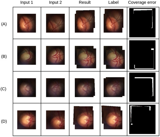
Figure 9.
Example results of the proposed method for low-resolution retinography image stitching. White areas indicate misaligned regions, where the result either incorrectly covers or fails to cover the reference image. (A–D) Test case.

Table 5.
Result by average metric for each method.
Still, it was found that the individualized regression strategy for each point was really useful for correcting inaccuracies and improving alignment, as exemplified in Figure 10, where it is easy to see that the multiple regression method can provide results closer to the label than single regression.
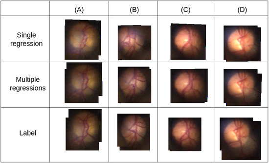
Figure 10.
Visual comparison of results before and after applying individual regressions. Columns (A–D) each represent a test case.
Figure 11 presents comparative examples of the 3 methods; it is evident in the first row, where FBF is not used during model training, that the model is unable to estimate a homography matrix that can be used to align the images. In the second line, with the single regression that used FBF during the training in some images, such as (A), (D), (E) and (F), it is possible to observe inferior alignment quality compared to the proposed method.
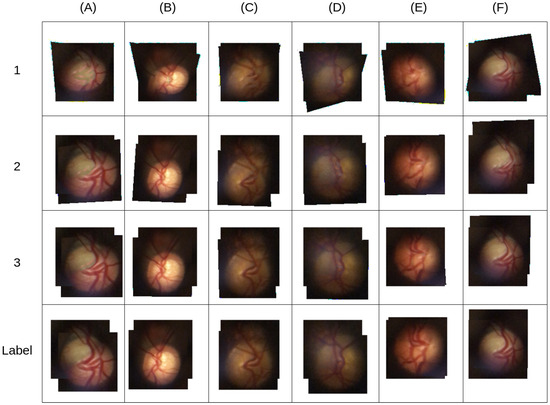
Figure 11.
Comparative examples of different methods for test cases (A–F). The numbered lines show the results of the following methods: (1) method proposed by [12], (2) method proposed by [12] with the addition of FBF, and (3) our method. The “Label” line contains the expected results.
Evaluating the proposed method on high-resolution images from the P subset of the FIRE dataset showed that the model could return a sufficiently accurate homography in 21 cases out of 49 image pairs. Most of the failures occurred with images with little overlap between them, an essential factor for accurate homography estimation. However, this is not a significant obstacle to the problem presented in this work since it is possible to use neighboring frames of the videos for stitching, ensuring sufficient overlap. Figure 12A shows a pair of images from subsection “P” of the FIRE dataset, where, with sufficient overlap between the pictures, the proposed method was able to estimate an approximate homography matrix. Figure 12B shows a pair of images with little overlap, in which the model could not estimate a homography matrix that aligned with the figures.
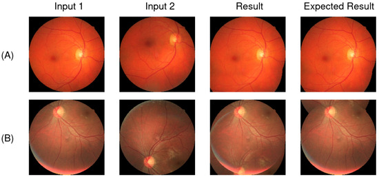
Figure 12.
Test case examples of the proposed method with the subset P from the FIRE dataset. (A) Case where there is enough overlap. (B) Not enough overlap.
4. Conclusions
This research proposed a homography estimation method for stitching low-resolution retinal images. The method could extract relevant features from the input images and calculate a correlation feature, enabling the alignment of retinal images.
From the results discussed, we can see that the introduction of the Fundus Blur Filter (FBF) into the training process of the homography estimation model brought important improvements with regard to image alignment accuracy. The increase in PSNR and SSIM, as well as the reduction in RMSE, indicate that the proposed model was able to consistently improve the quality of the reconstruction, outperforming previously tested methods. Although the method proved effective, especially in the D-EYE dataset, when compared to the method proposed by [12], improving the PSNR by 7.96 dB and achieves a 7.86% higher SSIM score, there are still challenges in situations where there is little overlap between the images, as observed in the FIRE dataset. Despite these limitations, we believe that the use of neighboring frames, as discussed, can mitigate some of these difficulties, ensuring sufficient overlap for proper alignment.
As this current approach requires manual intervention in selecting frames from the videos obtained through D-EYE, acting as a drawback for use in a clinical setting, future work is expected to overcome the identified limitations, aiming at automating the selection of sections of the area of interest in the video frames captured using D-EYE to develop automatic algorithms for ordering frames to enable alignment and stitching of multiple images. This will enable better visualization of the retina by reconstructing low-resolution retinographies in a panorama, helping ophthalmologists identify eye diseases early enough to treat them.
Author Contributions
Conceptualization, L.S., A.C. and J.A.; methodology L.S., M.A. and J.A.; validation, J.A. and M.A.; formal analysis, L.S. and J.A.; investigation, L.S. and J.A.; writing—original draft preparation, L.S. and J.A.; writing—review and editing, A.C., J.C., M.A. and G.B.; supervision, J.A.; project administration, J.A. All authors have read and agreed to the published version of the manuscript.
Funding
The authors acknowledge the Fundação para a Ciência e Tecnologia, IP (FCT) within the R&D Units Project Scope: UIDB/00319/2020 (ALGORITMI), Coordenação de Aperfeiçoamento de Pessoal de Nível Superior (CAPES), Brazil—Finance Code 001, Conselho Nacional de Desenvolvimento Científico e Tecnológico (CNPq), Brazil, and Fundação de Amparo à Pesquisa Desenvolvimento Científico e Tecnológico do Maranhão (FAPEMA) Brazil (Grant number 000527/2024) and Empresa Brasileira de Serviços Hospitalares (Ebserh) Brazil (Grant number 409593/2021-4) for providing financial support.
Institutional Review Board Statement
Not applicable.
Informed Consent Statement
Not applicable.
Data Availability Statement
The data presented in this study are available on request from the corresponding author.
Conflicts of Interest
The authors declare no conflicts of interest.
References
- WHO. World Report on Vision; World Health Organization: Geneva, Switzerland, 2019. [Google Scholar]
- Neto, A.; Camara, J.; Cunha, A. Evaluations of deep learning approaches for glaucoma screening using retinal images from mobile device. Sensors 2022, 22, 1449. [Google Scholar] [CrossRef]
- Pachade, S.; Porwal, P.; Thulkar, D.; Kokare, M.; Deshmukh, G.; Sahasrabuddhe, V.; Giancardo, L.; Quellec, G.; Mériaudeau, F. Retinal fundus multi-disease image dataset (RFMiD): A dataset for multi-disease detection research. Data 2021, 6, 14. [Google Scholar] [CrossRef]
- Resnikoff, S.; Lansingh, V.C.; Washburn, L.; Felch, W.; Gauthier, T.M.; Taylor, H.R.; Eckert, K.; Parke, D.; Wiedemann, P. Estimated number of ophthalmologists worldwide (International Council of Ophthalmology update): Will we meet the needs? Br. J. Ophthalmol. 2020, 104, 588–592. [Google Scholar] [CrossRef]
- Abdulhussein, D.; Abdul Hussein, M. WHO Vision 2020: Have we done it? Ophthalmic Epidemiol. 2023, 30, 331–339. [Google Scholar] [CrossRef]
- Pihlblad, M.S.; Stockslager, S. D-EYE: A portable and inexpensive option for fundus photography and videography in the pediatric population with telemedicine potential. J. Am. Assoc. Pediatr. Ophthalmol. Strabismus 2016, 20, e21. [Google Scholar] [CrossRef]
- Barritt, N.; Pilon, L.; MacLean, A.; Lin, A.; Cole, A.; Faruq, I.; Lakshminarayanan, V. Development and testing of a stabilization and image processing system for improvement of mobile fundus camera image quality. In Proceedings of the Novel Optical Systems, Methods, and Applications XXIII, SPIE, Virtual, 24 August–4 September 2020; Volume 11483, pp. 79–88. [Google Scholar]
- Correia, T.V.S. Detection and Mosaicing through Deep Learning Models for Low-Quality Retinal Images. Master’s Thesis, School of Technology and Management of the Polytechnic Institute of Leiria, Leiria, Portugal, 2023. Available online: https://iconline.ipleiria.pt/handle/10400.8/8892 (accessed on 7 August 2023).
- Liu, J.; Li, X.; Wei, Q.; Xu, J.; Ding, D. Semi-supervised keypoint detector and descriptor for retinal image matching. In Proceedings of the European Conference on Computer Vision, Tel Aviv, Israel, 23–27 October 2022; Springer: Berlin/Heidelberg, Germany, 2022; pp. 593–609. [Google Scholar]
- Hu, R.; Chalakkal, R.; Linde, G.; Dhupia, J.S. Multi-image stitching for smartphone-based retinal fundus stitching. In Proceedings of the 2022 IEEE/ASME International Conference on Advanced Intelligent Mechatronics (AIM), IEEE, Sapporo, Japan, 11–15 July 2022; pp. 179–184. [Google Scholar]
- Sedaghat, A.; Mokhtarzade, M.; Ebadi, H. Uniform Robust Scale-Invariant Feature Matching for Optical Remote Sensing Images. IEEE Trans. Geosci. Remote. Sens. 2011, 49, 4516–4527. [Google Scholar] [CrossRef]
- Nie, L.; Lin, C.; Liao, K.; Liu, M.; Zhao, Y. A view-free image stitching network based on global homography. J. Vis. Commun. Image Represent. 2020, 73, 102950. [Google Scholar] [CrossRef]
- DeTone, D.; Malisiewicz, T.; Rabinovich, A. Deep image homography estimation. arXiv 2016, arXiv:1606.03798. [Google Scholar]
- Huang, R.; Chang, Q.; Zhang, Y. Unsupervised Oral Endoscope Image Stitching Algorithm. J. Shanghai Jiaotong Univ. Sci. 2024, 29, 81–90. [Google Scholar] [CrossRef]
- Lin, T.Y.; Maire, M.; Belongie, S.; Bourdev, L.; Girshick, R.; Hays, J.; Perona, P.; Ramanan, D.; Zitnick, C.L.; Dollár, P. Microsoft COCO: Common Objects in Context. arXiv 2015, arXiv:1405.0312. [Google Scholar]
- Chopra, S.; Hadsell, R.; LeCun, Y. Learning a similarity metric discriminatively, with application to face verification. In Proceedings of the 2005 IEEE Computer Society Conference on Computer Vision and Pattern Recognition (CVPR’05), IEEE, San Diego, CA, USA, 20–26 June 2005; Volume 1, pp. 539–546. [Google Scholar]
- Chicco, D. Siamese neural networks: An overview. Artif. Neural Netw. 2021, 2190, 73–94. [Google Scholar]
- Hartley, R.; Zisserman, A. Multiple View Geometry in Computer Vision; Cambridge University Press: Cambridge, UK, 2003. [Google Scholar]
- Kang, L.; Wei, Y.; Xie, Y.; Jiang, J.; Guo, Y. Combining convolutional neural network and photometric refinement for accurate homography estimation. IEEE Access 2019, 7, 109460–109473. [Google Scholar] [CrossRef]
- O’shea, K.; Nash, R. An introduction to convolutional neural networks. arXiv 2015, arXiv:1511.08458. [Google Scholar]
- Szeliski, R. Computer Vision: Algorithms and Applications; Springer Nature: Berlin/Heidelberg, Germany, 2022. [Google Scholar]
- Liu, S.; Lu, Y.; Jiang, H.; Ye, N.; Wang, C.; Zeng, B. Unsupervised global and local homography estimation with motion basis learning. IEEE Trans. Pattern Anal. Mach. Intell. 2022, 45, 7885–7899. [Google Scholar] [CrossRef]
- Zhou, Q.; Li, X. STN-Homography: Direct estimation of homography parameters for image pairs. Appl. Sci. 2019, 9, 5187. [Google Scholar] [CrossRef]
- Wang, Z.; Yang, Z. Review on image-stitching techniques. Multimed. Syst. 2020, 26, 413–430. [Google Scholar] [CrossRef]
- Jagalingam, P.; Hegde, A.V. A review of quality metrics for fused image. Aquat. Procedia 2015, 4, 133–142. [Google Scholar] [CrossRef]
- Dissanayake, V.; Herath, S.; Rasnayaka, S.; Seneviratne, S.; Vidanaarachchi, R.; Gamage, C. Quantitative and Qualitative Evaluation of Performance and Robustness of Image Stitching Algorithms. In Proceedings of the 2015 International Conference on Digital Image Computing: Techniques and Applications (DICTA), Adelaide, Australia, 23–25 November 2015; pp. 1–6. [Google Scholar] [CrossRef]
- Wang, Z.; Bovik, A.C. Mean squared error: Love it or leave it? A new look at Signal Fidelity Measures. IEEE Signal Process. Mag. 2009, 26, 98–117. [Google Scholar] [CrossRef]
- Wang, Z.; Bovik, A.; Sheikh, H.; Simoncelli, E. Image quality assessment: From error visibility to structural similarity. IEEE Trans. Image Process. 2004, 13, 600–612. [Google Scholar] [CrossRef]
- Zhu, M.; Li, C.; He, X.; Xiao, X. Unsupervised deep learning image stitching model assisted with infrared images. In Proceedings of the International Conference on Algorithm, Imaging Processing, and Machine Vision (AIPMV 2023), Qingdao, China, 15–17 September 2023; SPIE: Bellingham, WA, USA, 2024; Volume 12969, pp. 249–255. [Google Scholar]
- Duan, H.; Min, X.; Sun, W.; Zhu, Y.; Zhang, X.P.; Zhai, G. Attentive deep image quality assessment for omnidirectional stitching. IEEE J. Sel. Top. Signal Process. 2023, 17, 1150–1164. [Google Scholar] [CrossRef]
- Ni, J.; Li, Y.; Ke, C.; Zhang, Z.; Cao, W.; Yang, S.X. A Fast Unsupervised Image Stitching Model Based on Homography Estimation. IEEE Sens. J. 2024, 24, 29452–29467. [Google Scholar] [CrossRef]
- The GIMP Development Team. GIMP: GNU Image Manipulation Program. Version 2.10.36. The GIMP Development Team. 2023. Available online: https://www.gimp.org (accessed on 10 February 2024).
- Hernandez-Matas, C.; Zabulis, X.; Triantafyllou, A.; Anyfanti, P.; Douma, S.; Argyros, A.A. FIRE: Fundus image registration dataset. Model. Artif. Intell. Ophthalmol. 2017, 1, 16–28. [Google Scholar] [CrossRef]
Disclaimer/Publisher’s Note: The statements, opinions and data contained in all publications are solely those of the individual author(s) and contributor(s) and not of MDPI and/or the editor(s). MDPI and/or the editor(s) disclaim responsibility for any injury to people or property resulting from any ideas, methods, instructions or products referred to in the content. |
© 2024 by the authors. Licensee MDPI, Basel, Switzerland. This article is an open access article distributed under the terms and conditions of the Creative Commons Attribution (CC BY) license (https://creativecommons.org/licenses/by/4.0/).