Article

Graph-Based Semi-Supervised Learning with Bipartite Graph for Large-Scale Data and Prediction of Unseen Data

1
Department of Computer Engineering, Shahid Rajaee Teacher Training University, Tehran 16785-163, Iran
2
Faculty of Computer Engineering, University of the Basque Country, 20018 San Sebastian, Spain
3
IKERBASQUE, Basque Foundation for Science, 48009 Bilbao, Spain
*
Author to whom correspondence should be addressed.
Information 2024, 15(10), 591; https://doi.org/10.3390/info15100591
Submission received: 15 July 2024 / Revised: 11 August 2024 / Accepted: 19 August 2024 / Published: 27 September 2024
(This article belongs to the Special Issue Feature Papers in Information in 2024–2025)

Abstract

:
Recently, considerable attention has been directed toward graph-based semi-supervised learning (GSSL) as an effective approach for data labeling. Despite the progress achieved by current methodologies, several limitations persist. Firstly, many studies treat all samples equally in terms of weight and influence, disregarding the potential increased importance of samples near decision boundaries. Secondly, the detection of outlier-labeled data is crucial, as it can significantly impact model performance. Thirdly, existing models often struggle with predicting labels for unseen test data, restricting their utility in practical applications. Lastly, most graph-based algorithms rely on affinity matrices that capture pairwise similarities across all data points, thus limiting their scalability to large-scale databases. In this paper, we propose a novel GSSL algorithm tailored for large-scale databases, leveraging anchor points to mitigate the challenges posed by large affinity matrices. Additionally, our method enhances the influence of nodes near decision boundaries by assigning different weights based on their importance and using a mapping function from feature space to label space. Leveraging this mapping function enables direct label prediction for test samples without requiring iterative learning processes. Experimental evaluations on two extensive datasets (Norb and Covtype) demonstrate that our approach is scalable and outperforms existing GSSL methods in terms of performance metrics.

Graphical Abstract

1. Introduction

The enhancement of classification performance through SSL, in circumstances where only a few costly labeled samples are available while plentiful unlabeled samples are easily obtained [1], has become a prominent research avenue and finds wide application in various real-world scenarios [2,3]. There were numerous intriguing proposals made to acquire knowledge from both labeled and unlabeled data, like transductive inference [4], co-training [5], and graph-based methods [6,7,8].
Graph construction plays an essential role in graph-based label propagation, as graphs provide information about the structure of the data manifold [9]. The success of GSSL methods can be attributed in part to the manifold assumption, which enhances the expressive power of graph structure [10]. While semi-supervised learning (SSL) models have shown promise in many areas, they can face challenges in certain scenarios. Next, we discuss the limitations encountered by several GSSL models:
  • Many of them are not able to predict the labels of unseen data. Consequently, due to the continuous updating and creation of data in the real world through the internet and social networks, these methods are difficult to apply to real-world problems.
  • The use of an n × n affinity matrix (where n is the number of samples) makes applying these methods to large databases computationally and memory-intensive.
  • Most of the existing models do not work based on weighted samples, and all samples have the same weight.
One major problem with semi-supervised learning models is their inability to estimate the labels of unseen data. With the expansion of the internet and social networks, data are rapidly generated and changing. Models that lack the ability to generalize to unseen data exhibit limited effectiveness in real-world applications. Therefore, using inductive models is necessary in many cases. Flexible Manifold Embedding (FME) [11] was designed to solve this problem. This method utilizes an objective function and linear mapping that enables the model to anticipate the labels of samples. Inspired by the FME model, Reduced Flexible Manifold Embedding (R-FME) was designed to work on large-scale datasets and to predict the labels of unseen data. To anticipate the labels of data, ref. [11] FME proposed a GSSL model that can also work on multi-view datasets.
The second limitation of GSSL methods is their scalability when dealing with large datasets. Traditional approaches to constructing affinity graphs involve calculating pairwise affinities between all nodes, leading to a computational complexity of O (n2). This quadratic time complexity becomes impractical as the size of the dataset increases. To address this issue, more efficient methods for constructing affinity matrices are needed. An affinity matrix is a square matrix used to represent the similarity or affinity between pairs of data points. Each entry in the matrix quantifies how similar or connected two data points are. In the context of a graph, the affinity matrix can be seen as the adjacency matrix of a weighted graph, where the weights represent the strength of the edges between nodes. For large-scale datasets, constructing a full affinity matrix can be computationally expensive and memory-intensive. Therefore, efficient strategies such as using approximations, leveraging sparsity, or employing bipartite graphs can significantly reduce the computational burden. These strategies enable more scalable and practical implementations of GSSL methods, making them more feasible for large datasets. A bipartite graph that shows the similarity between anchor points and data samples can be constructed with O (nm) order [12]. To generate anchor points, Random selection, and k-means generation are often the two available options. Using a set of clustering centers as anchor points, k-means clustering enhances the representativeness of the results [1]. R-FME and Fast FME (F-FME) [13] are two famous GSSL models that work on large-scale datasets. Graph-based learning is also used in large-scale unsupervised learning; for instance, the model proposed in [14] can cluster large-scale data using reinforcement learning technique.
The next limitation of GSSL methods is that not all samples have the same impact on the model. For example, samples near the decision boundary based on the idea of anchor points are more important than others [15,16]. Hence, their incorrect label estimation should have a large effect on the loss function. In recent studies, much attention has been paid to the weighted sample models. For example, studies [15,16] improved local and global consistency (LGC) performance using weighted samples obtained from k-means.
To address these limitations, we propose a graph-based semi-supervised learning approach that effectively handles large-scale datasets. Our model can predict unseen data via a bias term and a projection matrix.
In summary, this article is notable for the ensuing accomplishments:
  • A novel model based on graph-based semi-supervised learning is presented that uses anchor samples and can work on large-scale datasets with reasonable computational complexity.
  • By leveraging principal component analysis (PCA) for dimensionality reduction during data preprocessing, the proposed model efficiently extracts key features relevant to future prediction while simultaneously reducing computational runtime.
  • Similar to R-FME, the presented model can effectively handle data sampled from nonlinear manifold and provides a mapping for new data points to anticipate the labels of unseen data.
  • Using anchor points, we propose a weighting scheme that calculates weights for the nodes according to their topological location.
  • By weighting labeled samples, our model can reduce the effect of outliers and emphasizes samples close to decision borders, which enhance the performance of baseline methods.
The rest of this paper is organized as follows: Section 2 explains the related works in the area of GSSL, considering their benefits and drawbacks. In Section 3, we provide an overview of some fundamental preliminaries related to the proposed method. In Section 4, we discuss the proposed model and how it labels large-scale data. Section 5 provides a detailed description of the experimental results obtained using the proposed method. Finally, the conclusion of our paper can be found in Section 6.

2. Related Work

In this section, we introduce related work in graph-based learning. In recent years, graph-based semi-supervised and unsupervised learning approaches have been widely used across various areas. Although many models have been proposed, each suffers from some limitations.
Many studies focus on transductive learning on graphs. For unlabeled data prediction, ref. [17] proposes a harmonic function-based model. Ref. [18] builds a model on manifold assumptions, where nearby points and points on the same structure (cluster/manifold) are likely to share labels. Ref. [19] introduces a method for constructing a similarity matrix based on distance, where closer points have a higher similarity. Inspired by [19], ref. [20] develops a multi-view reinforcement learning model. Building on [20], ref. [14] addresses large-scale multi-view datasets using reinforcement learning and bipartite graphs for unlabeled data prediction. Refs. [12,21] propose graph-based spectral clustering models with anchor points identified by k-means to cluster large-scale data. Finally, models in [22,23,24] leverage bipartite graphs for large-scale unlabeled data prediction.
While previous studies utilizing graph-based semi-supervised learning have achieved success in various domains, many suffer from limitations in handling unseen data. Even though the Flexible Manifold Embedding (FME) method in [11] utilizes an objective function to predict the labels of unseen data, it incorporates all samples, hindering its scalability for large datasets. Subsequent studies, such as [9,25], addressed this limitation by proposing models that leverage dynamic graph construction techniques similar to those employed in [19]. Additionally, ref. [13] introduced two novel models, R-FME and F-FME, specifically designed for large-scale data prediction, handling both labeled and unlabeled data.
Although the studies mention above perform well on real-world datasets, none of them makes distinctions between data samples across the whole graph. It is worth saying that data near the decision boundary are more important than the others [15,16]. Recent studies have demonstrated that applying weights to samples can significantly enhance model accuracy, as it allows the model to focus on more relevant data points. In [16] Shannon’s self-information is used to generate weights for each node, which are then incorporated into the local and global consistency (LGC) model. The study in [15] uses the same idea with different uses of k-means and generates weights for data to help the model have better performance. With attention to topology imbalance in many different datasets, refs. [26,27] develop a model to generate weights for each labeled data point using a graph neural network. It is worth saying that most studies on weighing nodes do not achieve acceptable performance on large-scale datasets. The inability of these models to work on large datasets limits their applicability in industry.
Inspired by [20], the model proposed in [14] works on a large-scale multi-view dataset using reinforcement learning and bipartite graphs to predict the labels of unlabeled data. The authors in [12,21] propose a model to cluster large-scale data using graph and spectral clustering. In this model, anchor points are determined using k-means clustering, and then using a bipartite graph and spectral clustering, the model clusters the data. Moreover, the models in [22,23,24] predict the labels of unlabeled samples in large-scale datasets using bipartite graph.

3. Background

In this section, we provide an explanation for some of the mathematical notions used in the suggested method. Section 3.1 involves a concise explanation about the primary steps in SSL. In Section 3.2, we discuss a method called Weighted Samples-based Semi-Supervised Classification (WS3C) [16] and finally, in Section 3.3, we review the R-FME [13] algorithm.

3.1. Preliminaries

In this paper, we use bold capital characters for matrices, whereas bold lowercase letters represent vectors. Suppose we have n instances of data presented in matrix format
X = X l , X u = x 1 , x 2 , , x l , x l + 1 , , x l + u R d × n ,
where l , u , and n = l + u correspond to the number of labeled samples, unlabeled samples, and the total number of training samples, respectively. Also, d indicates the dimensionality of the samples. Moreover, we have a binary label matrix as
Y = Y l Y u = y 1 ; y 2 ; ; y l ; y l + 1 ; ; y n R n × c ,
where c is the number of classes, and Y i j = 1 if x i belongs to the j t h class and zero otherwise. Additionally, we have a soft-label matrix as
F = f 1 ; f 2 ; ; f n R n × c ,
where F i j indicates how probable it is for the sample x i to be a member of class j . Also, we have a graph as
G = { X , S } ,
where S R n × n is a directionless affinity matrix, and S i j offers evidence of the similarity between the two x i and x j nodes. In an anchor-based graph, similarities among all data points are measured with respect to a small set of m data points known as anchors. Given that m < < n , these similarities provide an efficient approximation of the large adjacency matrix using smaller-sized matrices.
For convenience, Table 1 illustrates the symbols used throughout this paper.

3.2. Review of WS3C Model

As discussed earlier, nodes closer to the decision boundary are more critical because they are more prone to incorrect label predictions. Therefore, it is essential to identify and assign greater importance to these nodes. In this section, we review the WS3C model and describe how it weights samples.
Consider X s R a × n as one feature subset of data where a < d . We cluster this subset and then define a clustering association graph as A R n × n where A i j = 1 if the two x i and x j samples are in the same cluster and zero otherwise. Assume that t clusterings are conducted on different feature subspaces of the data, with each clustering defining the association graph as A τ . In [16], the authors define A ˜ as
A ˜ = τ = 1 t A τ t ,
where A ˜ i j indicates the probability that two samples x i and x j are grouped in the same cluster across t clusterings. Closing value of A ˜ i j to 1 indicates that the two nodes are relatively similar (or close together) in the feature space. This suggests a high probability of them belonging to the same cluster. Conversely, a value close to 0 means that the nodes are likely not in the same cluster and are relatively far from each other. The closer A ˜ i j is to 0.5, the more difficult it is to determine whether the nodes should be in the same cluster or not.
The authors in [16] considered samples with A ˜ i j values close to 0.5 as samples with high importance and defined a hard-to-cluster index between x i and x j as
H i j = l o g 2 A ˜ i j l o g 2 1 A ˜ i j .
Using Equation (2), A ˜ i j values close to 0 and 1 will have small H i j   values, while A ˜ i j values close to 0.5 will have high H i j values.
In this case, the hard-to-cluster index between x i and x j is solely measured using H i j . To measure the index for each sample, we aggregate the index between x i and other samples as
η i = j = 1 n H i j .
High values for η i indicate that a sample is on the border, while lower values suggest that it is inside a cluster.

3.3. Review of R-FME

As previously mentioned, the FME method [11] suffers from a key drawback: its computational cost scales cubically with the number of samples. Therefore, when dealing with large-scale datasets, the algorithm mandates extensive memory allocation and presents considerable computational overhead. The authors in [13] addressed this problem by adopting anchor points in the objective function of FME and called their method Reduced FME (R-FME).
Consider the matrix Z = z 1 , z 2 , , z m R m × d as m anchor points, where m < < n . Also, we have the affinity matrix B R n × m , which shows the similarity between n training samples and the m anchor points. In our research, we leveraged the K-Nearest Neighbor (KNN) method to compute matrix B . Specifically, we set k to 10, and the similarity between data points was determined using a Gaussian function. Additionally, the similarity matrix between the anchors can be calculated using W ˜ = B T B . Consider that the estimated labels for the anchors are stored in A R m × c . Hence, the label of the training set can be calculated using
F = B A .
The objective function of the R-FME algorithm is given by
A * , Q * , b * = m i n A , Q , b Tr   A T L A + T r ( B A Y ) T U ( B A Y ) + μ Q 2 + γ Z T Q + 1 b T A 2 ,
where L is the laplacian matrix of anchor–anchor graph, U signifies the diagonal matrix with l non-zero diagonal elements for the labeled samples, projection matrix is shown as Q , b is the shift vector, and μ and γ are balance parameters.
The first term is the label smoothness of the anchors, the second term is the label fitting term for the labeled samples, the third term is the regularization of the projection matrix, and the forth one is the error in label estimation over the anchors using the projection matrix.
The mathematical formulations for Equation (5) provide closed-form solutions for A , Q , and b . As described in [13], the solutions are as
A = [ L ˜ + B T U B + μ H a μ H a Z T Z H a Z T + γ I 1 Z H a 1 B T U Y ,
Q = Z H a Z T + γ I 1 Z H a A ,
and
b = 1 m A T 1 Q T Z 1 ,
where L ˜ is the normalized Laplacian graph calculated as L ˜ = I D ˜ 1 / 2 W ˜ D ˜ 1 / 2 , with W ˜ = B T B and D ˜ R m × m being the diagonal matrix with diagonal elements D ˜ i i = j W ˜ i j , i .
Table 2 lists the full names of the acronyms used in this paper.

4. Proposed Model

In this section, we explain the proposed model and explain each part of it. In Section 4.1, we explain how we applied the weighting scheme to large-scale datasets, and in Section 4.2, we explain the proposed objective function.

4.1. Weighting Labeled Samples

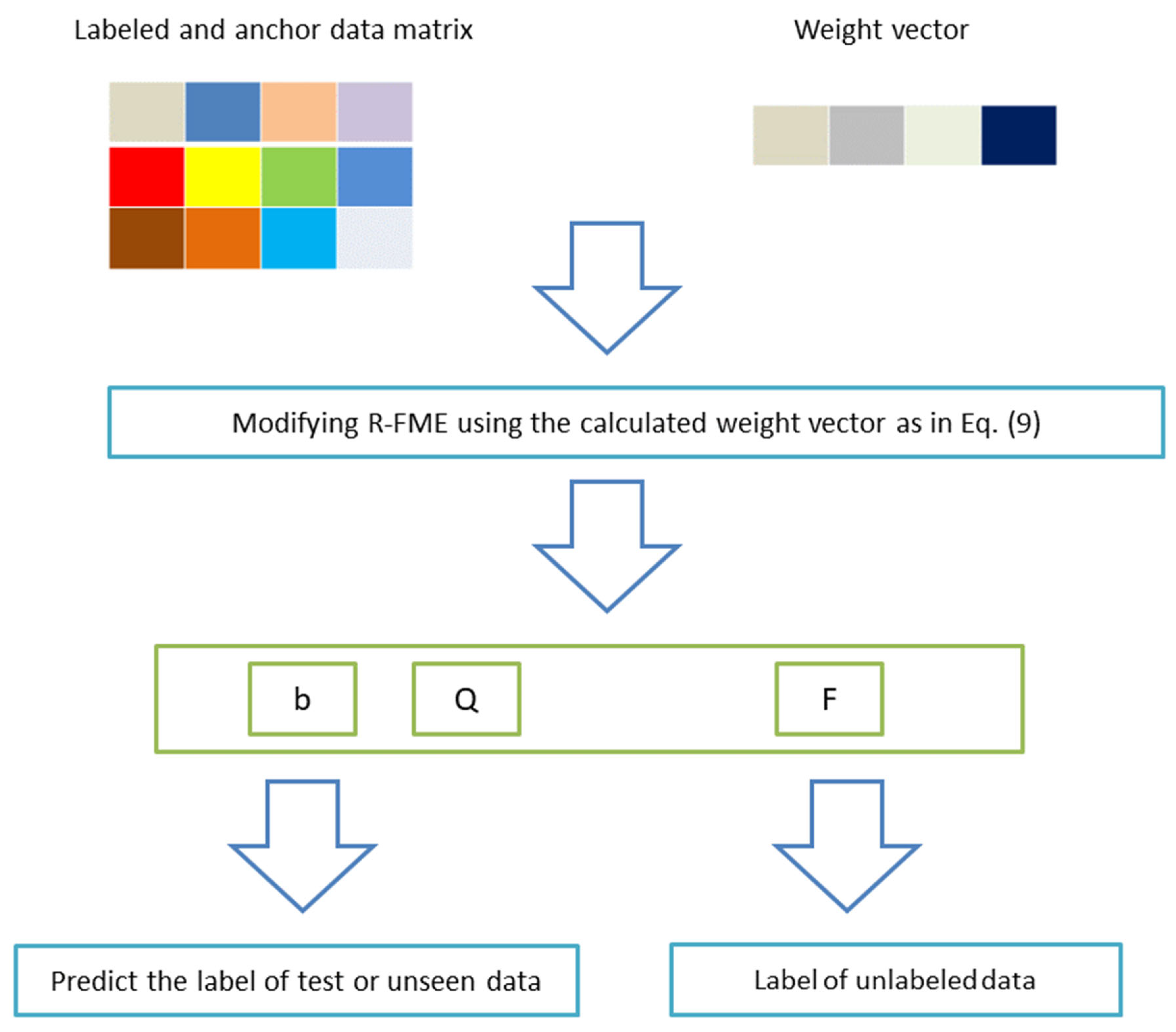
The node weighting idea proposed in [16] was applied to small datasets. Due to the use of a clustering association matrix with dimensionality n × n , it is challenging to apply this approach directly to large-scale datasets. In the following, we explain how we can make this idea adaptable to large-scale datasets. What we need is to weigh the labeled samples in the training set. However, the number of unlabeled samples is large, and it is not efficient to use them all in the weighting algorithm. Therefore, instead of using the entire dataset in the WS3C algorithm, we use the labeled data and m anchor points for the unlabeled set of data and construct the data matrix P = X l Z . Instead of constructing a clustering association graph with all nodes, we construct a graph containing only labeled data and anchors. Thus, the dimensionality of the clustering graph becomes m + l × m + l and m < < n . From this, we can calculate a weight for each labeled data and consequently have a vector containing weights for all labeled samples. The next step is to apply these weights to the R-FME objective function. Figure 1 shows the flowchart of modified WS3C algorithm.

4.2. Proposed Algorithm

One of the main limitations of the R-FME model is that it does not differentiate between samples close to the decision boundaries and those far from them and assigns equal weights to all samples. In other words, samples close to the decision boundaries are weighted the same as those farther away. To address this limitation, we propose a modified objective function that assigns topologically related weights to the labeled samples. We achieve this by changing the label fitting error term, which is the second term in Equation (5). As explained in Equation (5), the diagonal U matrix has l non-zero elements for labeled samples. As explained in Section 4.1, we calculate a weight value v i for each labeled node x i . Consequently, we change the U matrix values and use the calculated weights by setting
U i i = v i .
For each labeled sample x i , this results in different weights for each labeled sample based on its topological location.
The next step is to solve the proposed objective function. Since the vector v is calculated separately and fixed in our objective function, the solution to the proposed method is similar to that of the R-FME method, except that the U matrix in the proposed framework is computed using Equation (9).
Figure 2 shows the flowchart of our proposed model. Moreover, Table 3 shows the algorithm of the proposed method.
The proposed method contains two algorithms: the weighting method and the R-FME algorithm. Since the proposed method first applies the weighting method and then the R-FME algorithm, the computational complexity of the proposed method is the summation of two computational complexities of the W3SC and R-FME algorithms. In this case, the computational complexity of the proposed method is
O ( t m + l × m × d × r + t m + l 2 + ( m + l ) 3 ) + O ( n m 2 + m 3 + m 2 d + m d 2 + d 3 ) .

5. Experiment

In this section, we examine the efficacy of our proposed approach on two large-scale datasets. In Section 5.1, the original datasets employed in our studies are described, alongside the adopted preprocessing steps. Section 5.2 provides a detailed evaluation of parameter tuning and identifies the optimal parameters for the proposed model. A detailed analysis of how the proposed method performs compared to other state-of-the-art algorithms is provided in Section 5.3.

5.1. Datasets

The following overview provides a brief description of the Norb and CoverType large-scale datasets employed in this work.
Norb: It stands for NYU Object Recognition Benchmark, and it is a collection of images and labels for generic object recognition in images. The dataset contains objects belonging to 5 categories: four-legged animals, human figures, airplanes, trucks, and cars. There are 10 instances of each category, 5 for training and 5 for testing. The combined count of photo pairs for testing and training reaches 24,300 in total. An example of images from the Norb dataset is given in Figure 3.
Figure 3. Example images from the Norb dataset [31].
Information 15 00591 g003
CoverType: The dataset has 54 features, including 10 numerical variables such as elevation, slope, and distance to water sources, and 44 binary variables indicating the presence or absence of certain wilderness areas and soil types [32]. The Covertype dataset is a popular benchmark for multiclass classification and semi-supervised learning methods. The Covertype dataset is highly imbalanced. The majority class (Lodgepole Pine) accounts for almost half of the samples, while the minority class (Cottonwood/Willow) accounts for less than 1% [32]. Similar to [13], we select 80% of the data for training and 20% for testing.
For each database, we choose o samples from each class in the training set as labeled samples, and the rest are set as unlabeled samples. For the Norb database, we have o = 5 ,   7 ,   a n d   10 , and for the CoverType database, we have o = 30 ,   50 ,   a n d   70 . We aimed for unbiased results regardless of the way the data were arranged, thus we formed 20 diverse combinations of labeled and unlabeled data. Furthermore, our approach involves utilizing PCA to decrease the dimensionality of the samples down to 50. In this case, our model can focus on important features and work faster with lower computational processing.
Moreover, we need anchor points as data representatives. For simplicity, we use the k-means clustering method to generate anchor points. In our study, similar to [13], we separate the data into 1000 clusters and use their centroids as anchor points. Table 4 shows a brief description of the datasets used in the model.

5.2. Parameter Tuning

In this section, we first discuss the parameters that need to be tuned in the proposed model. The proposed method has four parameters: the two balance parameters of the R-FME method (i.e., μ and γ ) and two parameters for the WS3C model, namely the percent of the feature subset (i.e., p ) and the number of clusters (i.e., t ) .
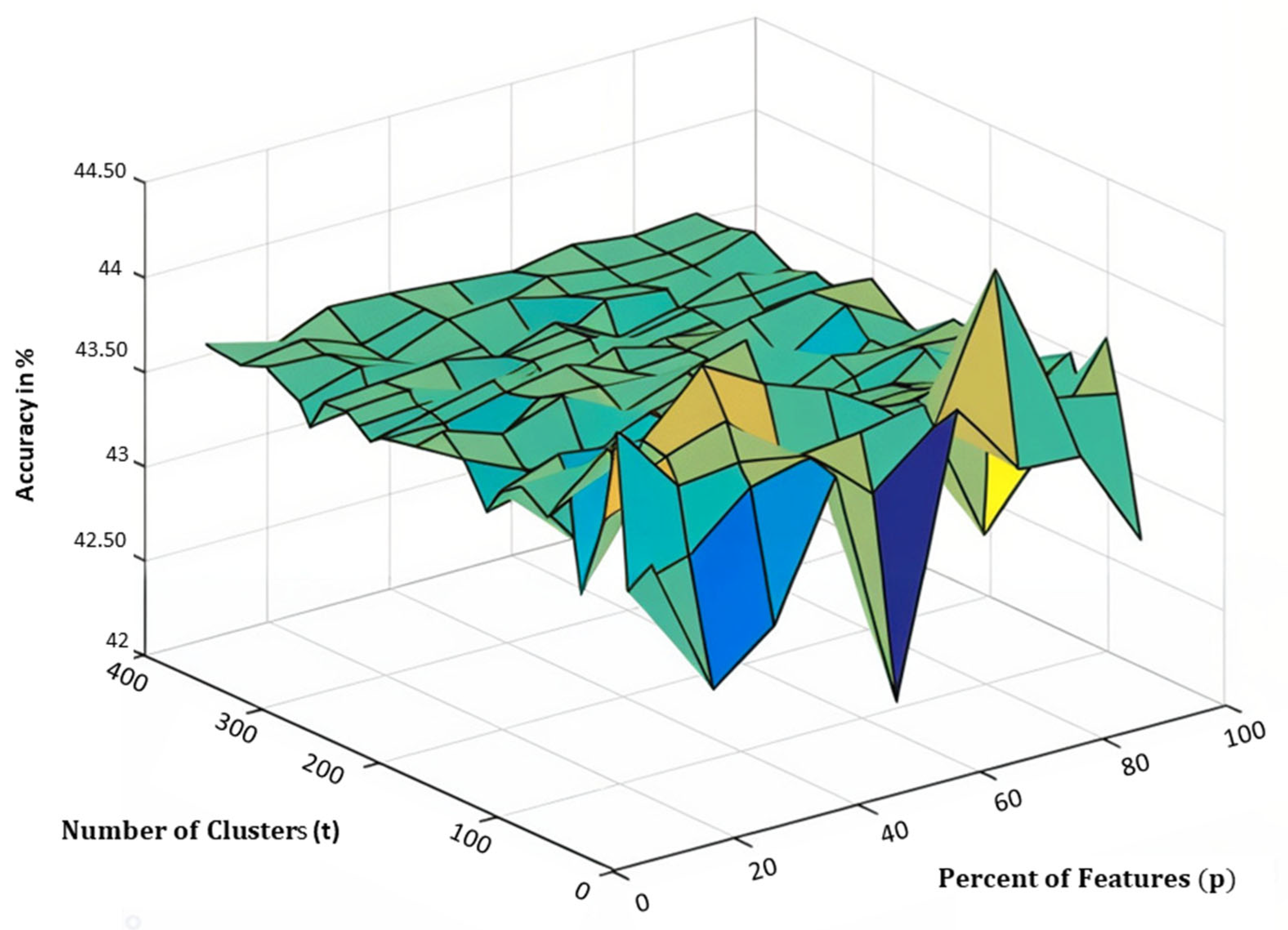
To find the best parameters for each database, we select a subset of data and perform a grid search. We vary p from 10% to 90% and t from 20 to 350, and then we calculate the accuracy of the proposed method. The reported accuracy is calculated as the percentage of correctly classified samples over the whole number of classifications. Figure 4 and Figure 5 show the accuracy versus the parameters for the Norb dataset, with 10 labeled samples per class for the train and test samples, respectively. Figure 4 shows a much flatter and more consistent surface with only one prominent peak. This suggests that the algorithm is highly stable across most parameter combinations, with a specific setting that leads to a slightly higher accuracy. The overall consistency in the second plot highlights the algorithm’s robustness and suggests that it can maintain high performance with minimal sensitivity to the changes in parameters. In Figure 5, however, the landscape is more uneven, with multiple peaks and valleys, suggesting that while the algorithm performs consistently across most settings, certain combinations of parameters can lead to significant drops in accuracy. This indicates that while the algorithm is resilient, there are particular parameter settings that may result in suboptimal performance.
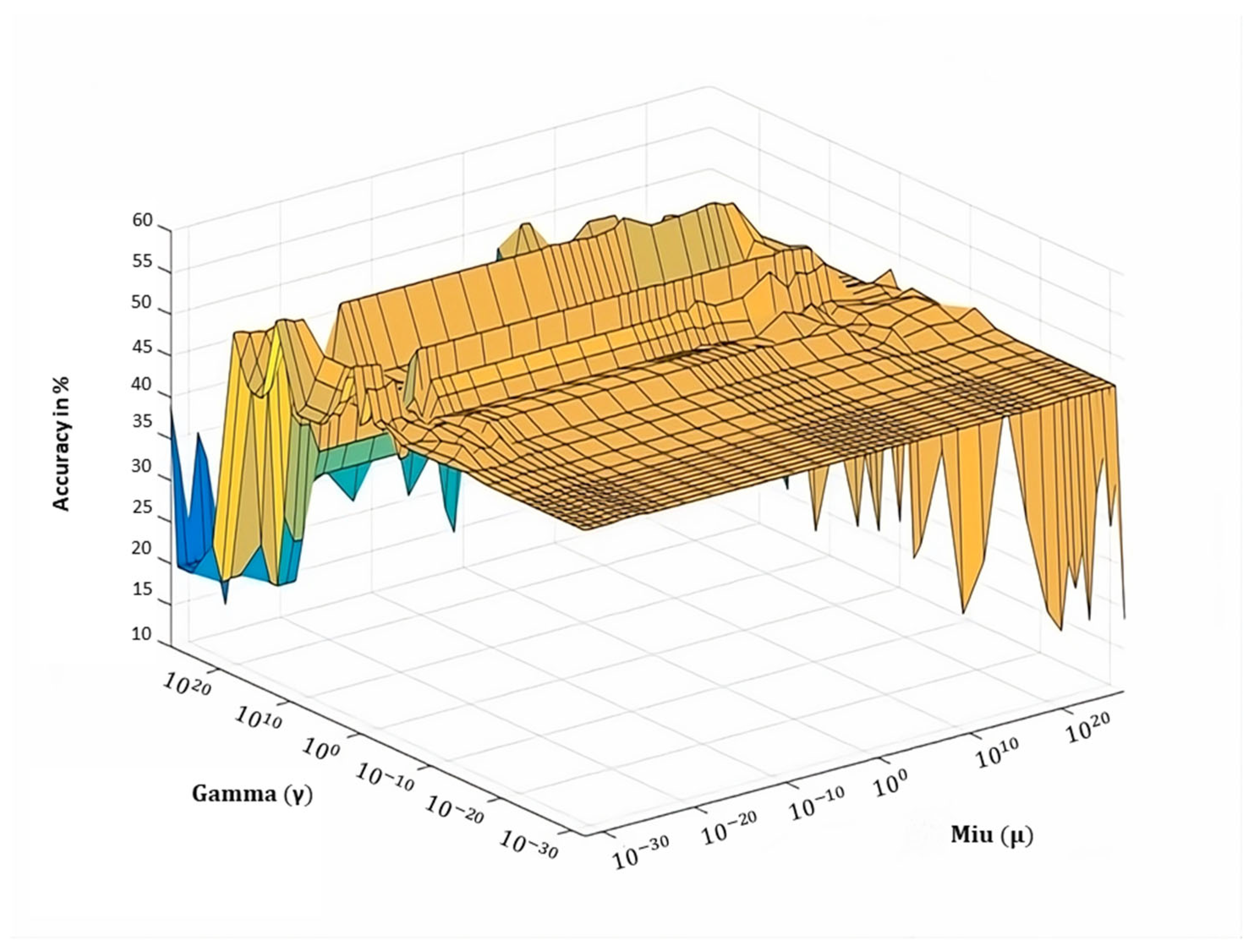
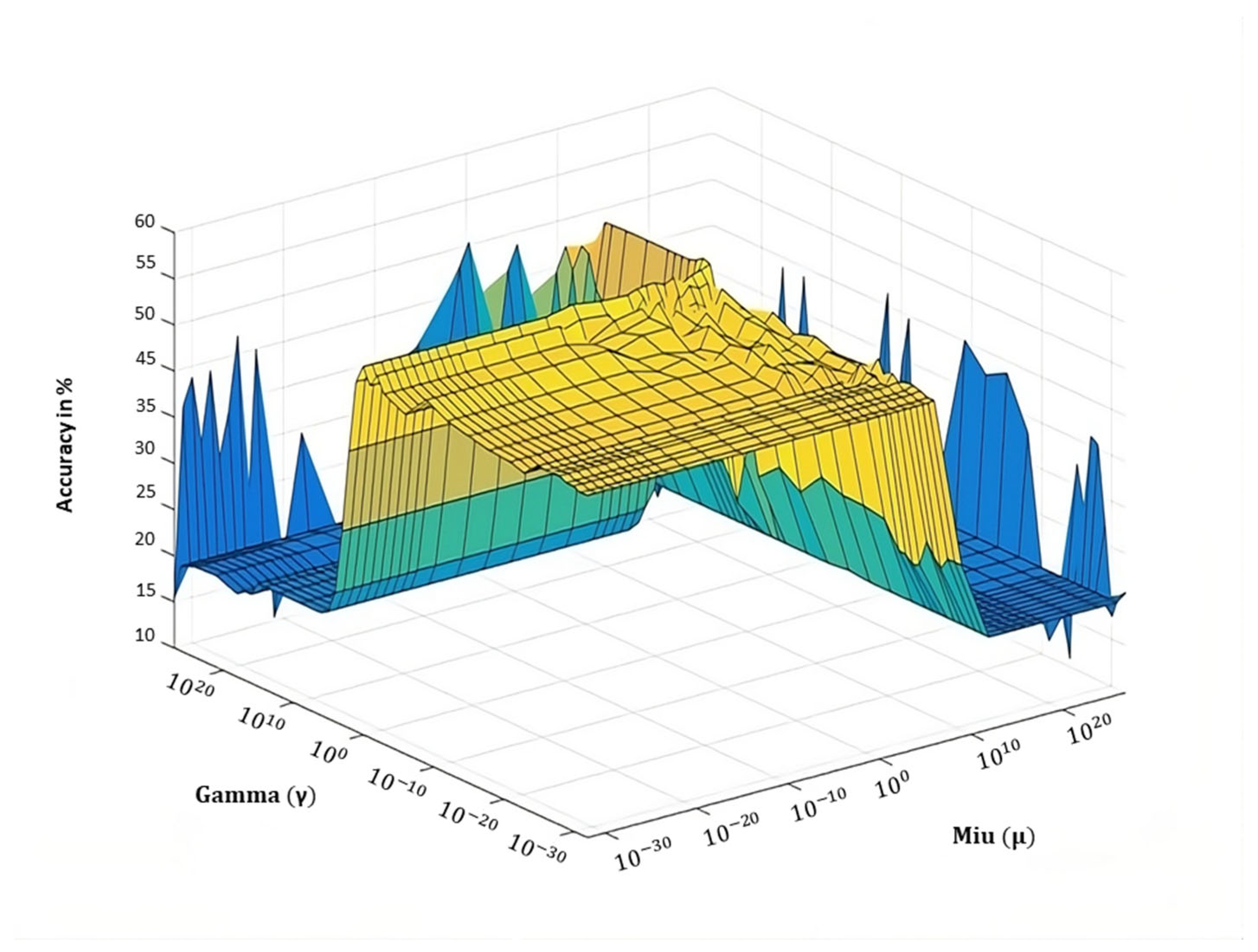
In the second experiment, we find the best values for μ and γ . Similar to the previous experiment, we perform a grid search and evaluate the model’s accuracy based on different values of μ   a n d   γ , for unlabeled data and test samples. Like before, we vary both μ and λ from 10 30 to 10 20 , and then we calculate the accuracy of the proposed method. Figure 6 and Figure 7 show the model results for the training and test datasets for the Norb dataset with o = 10 , respectively. Figure 8 and Figure 9 show the model results for the training and test data of the Covertype with o = 30 , respectively.
Based on our grid search results, the optimal parameters are outlined in Table 5 for the Norb dataset and in Table 6 for the CoverType database. These tables present the results of parameter tuning across various numbers of labeled samples per class. Each table specifies the type of data split: train for model training and test for performance evaluation. The “Labeled samples per class” column indicates the number of labeled examples from each class used during training (e.g., 10 labeled samples per class in the first row). The “Number of clusters” column denotes the number of clusters used in k-means clustering. The “Percent of feature subset” column shows the percentage of features utilized in the training process. Additionally, the “μ value” and “γ value” columns represent the balance parameters of the R-FME method employed in the model.

5.3. Comparison with Other Methods

To further evaluate the performance of the proposed model, in this section, we compare the accuracy of our model with that of state-of-the-art algorithms that work on large-scale datasets. In this case, as we discussed before for the Norb dataset, we set O = 5 , 7 ,   a n d   10 as the number of labeled nodes per class and set o = 30 , 50 ,   a n d   70 for the Cover type dataset. To eliminate the impact of randomization of labeled samples on the classification results, we generate 20 randomized selections of unlabeled and labeled data and report the average accuracy rate along with its standard deviation. In Table 7 and Table 8, we compare the model accuracy of the proposed model with other state-of-the-art algorithms on the Norb and Covertype datasets. All transductive methods, including AnchorGraphReg (AGR) [22], Efficient Anchor Graph Regularization (EAGR) [23], Minimax Label Propagation (MMLP) [28], and Minimum Tree Cut (MTC) [29], cannot predict labels for unseen test samples. AGR tackles scalability challenges in graph-based semi-supervised learning by leveraging a minimal set of anchor points, which allows for efficient nonparametric regression and accurate label prediction across large datasets [22]. EAGR introduces Efficient Anchor Graph Regularization (EAGR), an enhanced framework designed to address the limitations of Anchor Graph Regularization (AGR) by improving both local weight estimation and adjacency matrix effectiveness for large datasets [23]. MMLP introduces a path-based semi-supervised learning (SSL) framework that efficiently propagates labels through a minimal set of critical paths between labeled and unlabeled nodes, leveraging minimax paths to enhance performance [28]. MTC presents Minimum Tree Cut, a novel graph-based transductive classification method designed to address scalability and robustness issues in large-scale data by approximating the graph with a spanning tree and minimizing the cut size with a linear-time algorithm [29]. LapRLS introduces Linear Manifold Regularization, a method designed to enhance large-scale semi-supervised learning by applying linear manifold techniques to improve the handling of partially classified training data [30]. F-FME enhances scalability by utilizing anchor points for efficient graph construction and provides a simplified closed-form solution, demonstrating significant improvements in both computational efficiency and learning performance in large-scale semi-supervised learning scenarios [13]. R-FME achieves linear scalability in both time and space by constructing the graph adjacency matrix using a small number of anchor points, resulting in a simplified solution and demonstrating enhanced effectiveness and efficiency in large-scale graph-based semi-supervised learning [13].
As we observed, the proposed method has better accuracy than other models. Compared to the R-FME method, the accuracy is significantly enhanced by the weighted technique, which highlights the importance of incorporating the weight of labeled samples under the given scenario. Also, the proposed method has a lower standard deviation in contrast to the R-FME method.
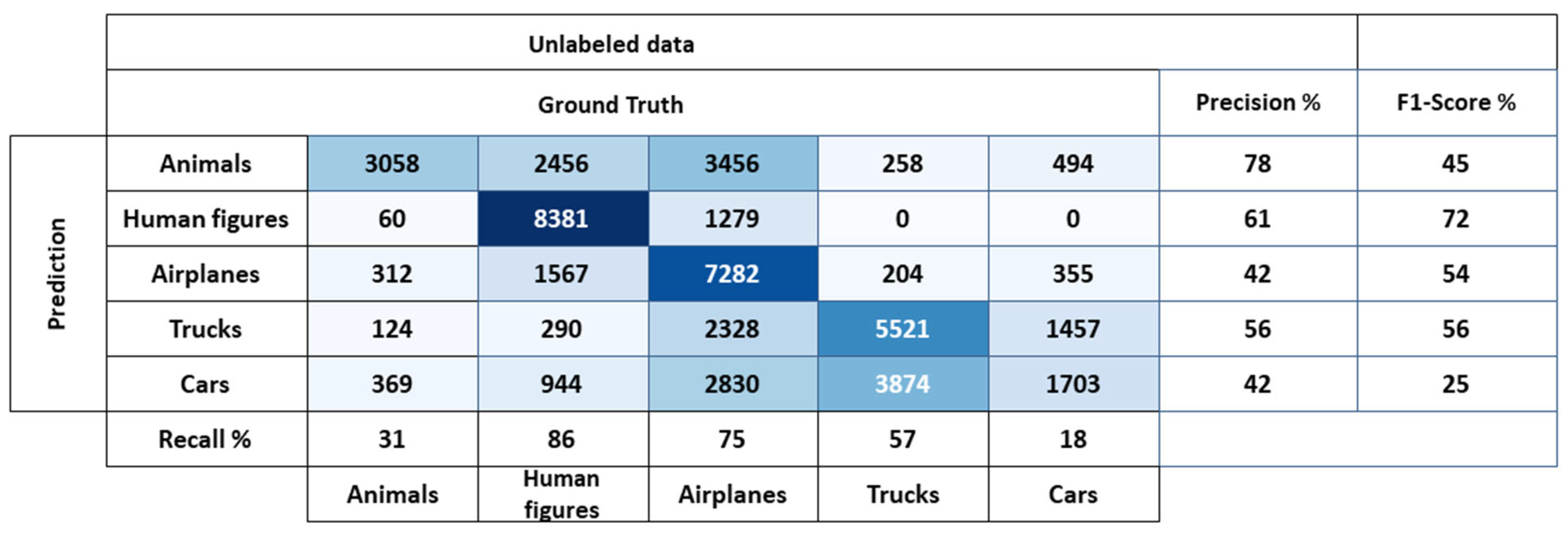
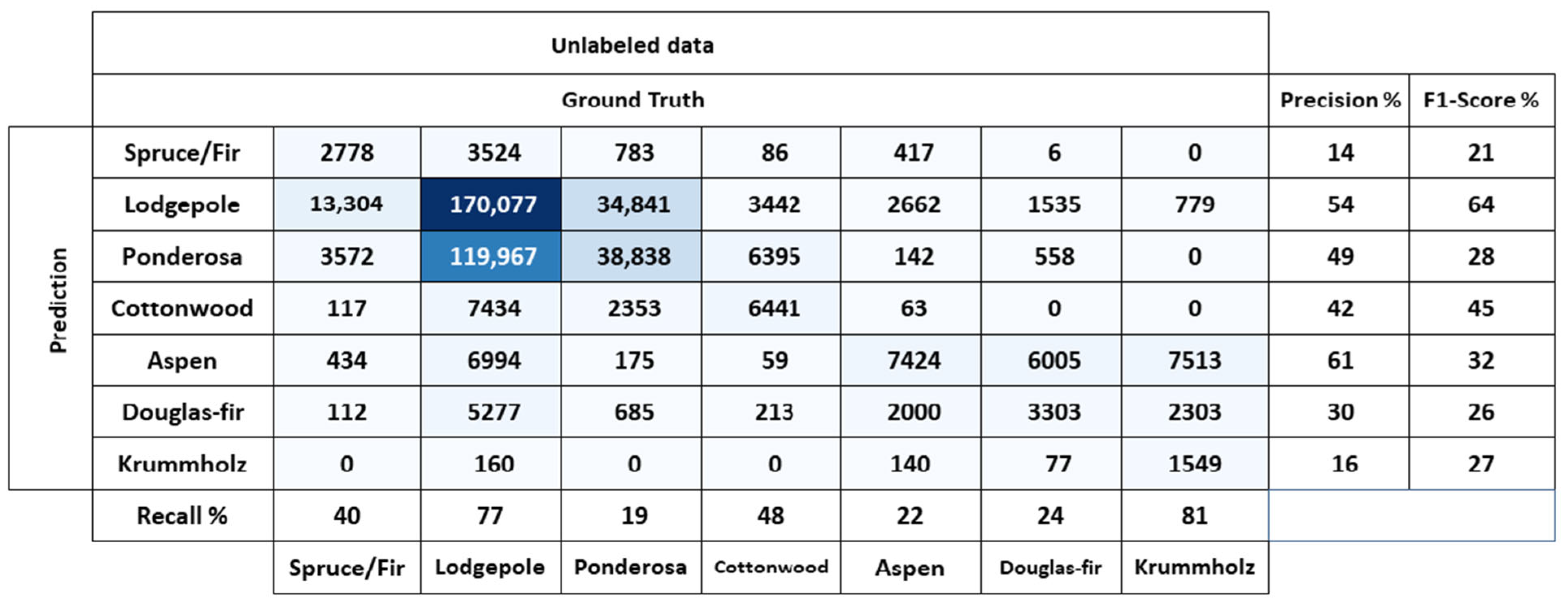
To measure the performance of classification models, which aim to predict a categorical label for each input instance in Figure 10 and Figure 11, we show a Confusion Matrix for the Norb with o = 5 and the Covertype dataset with o = 30. The matrix displays the number of true positive (TP), true negative (TN), false positive (FP), and false negative (FN) produced by the model on the test data. To have a better evaluation of our model, in Figure 10 and Figure 11, we show other parameter responses such as the F1-Score, Recall, and Precision.

6. Conclusions

This paper presents a novel graph-based semi-supervised learning (GSSL) method specifically designed for large-scale datasets. Our method builds upon the Reduced Flexible Manifold Embedding (R-FME) framework and introduces several key innovations that address the limitations of existing GSSL approaches.

6.1. Scalability

Our approach effectively scales to large datasets by employing a reduced-complexity graph construction using anchor points. This strategy mitigates the computational and memory constraints typically associated with large-scale GSSL methods.

6.2. Weighted Node Importance

We introduce a differential weighting scheme for label nodes based on their topological proximity to class boundaries. This novel feature enhances classification performance by prioritizing nodes that are critical for defining class boundaries, which is a significant advancement over traditional methods that treat all nodes uniformly.

6.3. Unseen Data Prediction

Our method incorporates a mechanism to predict labels for previously unseen data, addressing a major limitation of current models. This capability extends the applicability of our approach to dynamic and evolving datasets encountered in real-world scenarios.

6.4. Performance

Comprehensive evaluations of benchmark datasets demonstrate that our method achieves state-of-the-art performance in terms of accuracy and computational efficiency, surpassing existing GSSL techniques.
Future work will focus on further refining our model by reducing the number of hyperparameters and exploring various weighting strategies. Additionally, integrating our approach with Graph Neural Networks (GNNs) holds potential for further enhancing performance in large-scale data labeling tasks. Our findings underscore the efficacy of weighted models in advancing GSSL methodologies and suggest promising avenues for future research.

Author Contributions

Conceptualization, M.A. and A.B.; Methodology, M.A., A.B. and F.D.; Software, M.A.; Validation, M.A. and A.B.; Formal analysis, M.A. and A.B.; Investigation, M.A. and A.B.; Resources, M.A., A.B. and F.D.; Data curation, A.B.; Writing—original draft, M.A., A.B. and F.D.; Writing—review & editing, M.A., A.B. and F.D.; Visualization, M.A. and A.B.; Supervision, A.B.; Project administration, A.B.; Funding acquisition, A.B. and F.D. All authors have read and agreed to the published version of the manuscript.

Funding

This research has been partially supported by Shahid Rajaee Teacher Training University under grant number 4891 and by the University of the Basque Country UPV/EHU grant GIU23/022, and by the Ministerio de Ciencia, Innovación y Universidades, AEI, under grant PID2021-126701OB-I00.

Institutional Review Board Statement

Not applicable.

Informed Consent Statement

Not applicable.

Data Availability Statement

In this research we used two publicly available databases namely Norb and Covertype that can download the data from the provided addresses. NORB Dataset: Downloaded on August 2020 from: https://cs.nyu.edu/~ylclab/data/norb-v1.0 (accessed on 11 August 2024).; Covertype Dataset: Downloaded on August 2020 from: https://archive.ics.uci.edu/dataset/31/covertype (accessed on 11 August 2024).

Conflicts of Interest

The authors declare no conflict of interest.

References

  1. He, F.; Nie, F.; Wang, R.; Li, X.; Jia, W. Fast semisupervised learning with bipartite graph for large-scale data. IEEE Trans. Neural Netw. Learn. Syst. 2019, 31, 626–638. [Google Scholar] [CrossRef] [PubMed]
  2. Cheng, L.; Pan, S.J. Semi-supervised domain adaptation on manifolds. IEEE Trans. Neural Netw. Learn. Syst. 2014, 25, 2240–2249. [Google Scholar] [CrossRef] [PubMed]
  3. Xiang, S.; Nie, F.; Zhang, C. Semi-supervised classification via local spline regression. IEEE Trans. Pattern Anal. Mach. Intell. 2010, 32, 2039–2053. [Google Scholar] [CrossRef]
  4. Joachims, T. Transductive inference for text classification using support vector machines. In Proceedings of the International Conference on Machine Learning (ICML), Bled, Slovenia, 27–30 June 1999. [Google Scholar]
  5. Blum, A.; Mitchell, T. Combining labeled and unlabeled data with co-training. In Proceedings of the Eleventh Annual Conference on Computational Learning Theory, Madison, WI, USA, 24–26 July 1998. [Google Scholar]
  6. Nie, F.; Xiang, S.; Liu, Y.; Zhang, C. A general graph-based semi-supervised learning with novel class discovery. Neural Comput. Appl. 2010, 19, 549–555. [Google Scholar] [CrossRef]
  7. Nie, F.; Shi, S.; Li, X. Semi-supervised learning with auto-weighting feature and adaptive graph. IEEE Trans. Knowl. Data Eng. 2019, 32, 1167–1178. [Google Scholar] [CrossRef]
  8. Wang, Z.; Zhang, L.; Wang, R.; Nie, F.; Li, X. Semi-supervised learning via bipartite graph construction with adaptive neighbors. IEEE Trans. Knowl. Data Eng. 2022, 35, 5257–5268. [Google Scholar] [CrossRef]
  9. Ziraki, N.; Dornaika, F.; Bosaghzadeh, A. Multiple-view flexible semi-supervised classification through consistent graph construction and label propagation. Neural Netw. 2022, 146, 174–180. [Google Scholar] [CrossRef] [PubMed]
  10. Song, Z.; Yang, X.; Xu, Z.; King, I. Graph-based semi-supervised learning: A comprehensive review. IEEE Trans. Neural Netw. Learn. Syst. 2022, 34, 8174–8194. [Google Scholar] [CrossRef]
  11. Nie, F.; Xu, D.; Tsang, I.W.-H.; Zhang, C. Flexible manifold embedding: A framework for semi-supervised and unsupervised dimension reduction. IEEE Trans. Image Process. 2010, 19, 1921–1932. [Google Scholar] [PubMed]
  12. Li, Y.; Nie, F.; Huang, H.; Huang, J. Large-scale multi-view spectral clustering via bipartite graph. In Proceedings of the AAAI Conference on Artificial Intelligence, Austin, TX, USA, 25–30 January 2015. [Google Scholar]
  13. Qiu, S.; Nie, F.; Xu, X.; Qing, C.; Xu, D. Accelerating flexible manifold embedding for scalable semi-supervised learning. IEEE Trans. Circuits Syst. Video Technol. 2018, 29, 2786–2795. [Google Scholar] [CrossRef]
  14. Li, L.; He, H. Bipartite graph based multi-view clustering. IEEE Trans. Knowl. Data Eng. 2020, 34, 3111–3125. [Google Scholar] [CrossRef]
  15. Aromal, M.; Rasool, A.; Dubey, A.; Roy, B. Optimized Weighted Samples Based Semi-supervised Learning. In Proceedings of the 2021 Second International Conference on Electronics and Sustainable Communication Systems (ICESC), Coimbatore, India, 4–6 August 2021. [Google Scholar]
  16. Chen, X.; Yu, G.; Tan, Q.; Wang, J. Weighted samples based semi-supervised classification. Appl. Soft Comput. 2019, 79, 46–58. [Google Scholar] [CrossRef]
  17. Zhu, X.; Ghahramani, Z.; Lafferty, J.D. Semi-supervised learning using gaussian fields and harmonic functions. In Proceedings of the 20th International Conference on Machine Learning (ICML-03), Washington, DC, USA, 21–24 August 2003. [Google Scholar]
  18. Zhou, D.; Bousquet, O.; Lal, T.; Weston, J.; Schölkopf, B. Learning with local and global consistency. Adv. Neural Inf. Process. Syst. 2003, 16. [Google Scholar]
  19. Nie, F.; Cai, G.; Li, X. Multi-view clustering and semi-supervised classification with adaptive neighbours. In Proceedings of the AAAI Conference on Artificial Intelligence, San Francisco, CA, USA, 4–9 February 2017. [Google Scholar]
  20. Wang, H.; Yang, Y.; Liu, B. GMC: Graph-based multi-view clustering. IEEE Trans. Knowl. Data Eng. 2019, 32, 1116–1129. [Google Scholar] [CrossRef]
  21. Yang, X.; Yu, W.; Wang, R.; Zhang, G.; Nie, F. Fast spectral clustering learning with hierarchical bipartite graph for large-scale data. Pattern Recognit. Lett. 2020, 130, 345–352. [Google Scholar] [CrossRef]
  22. Liu, W.; He, J.; Chang, S.-F. Large graph construction for scalable semi-supervised learning. In Proceedings of the 27th International Conference on Machine Learning (ICML-10), Haifa, Israel, 21–24 June 2010. [Google Scholar]
  23. Wang, M.; Fu, W.; Hao, S.; Tao, D.; Wu, X. Scalable semi-supervised learning by efficient anchor graph regularization. IEEE Trans. Knowl. Data Eng. 2016, 28, 1864–1877. [Google Scholar] [CrossRef]
  24. Wang, Z.; Wang, L.; Chan, R.; Zeng, T. Large-scale semi-supervised learning via graph structure learning over high-dense points. arXiv 2019, arXiv:1912.02233. [Google Scholar]
  25. Bahrami, S.; Dornaika, F.; Bosaghzadeh, A. Joint auto-weighted graph fusion and scalable semi-supervised learning. Inf. Fusion 2021, 66, 213–228. [Google Scholar] [CrossRef]
  26. Chen, D.; Lin, Y.; Zhao, G.; Ren, X.; Li, P.; Zhou, J.; Sun, X. Topology-imbalance learning for semi-supervised node classification. Adv. Neural Inf. Process. Syst. 2021, 34, 29885–29897. [Google Scholar]
  27. Sun, Q.; Li, J.; Yuan, H.; Fu, X.; Peng, H.; Ji, C.; Li, Q.; Yu, P.S. Position-aware structure learning for graph topology-imbalance by relieving under-reaching and over-squashing. In Proceedings of the 31st ACM International Conference on Information & Knowledge Management, Atlanta, GA, USA, 17–22 October 2022. [Google Scholar]
  28. Kim, K.-H.; Choi, S. Label propagation through minimax paths for scalable semi-supervised learning. Pattern Recognit. Lett. 2014, 45, 17–25. [Google Scholar] [CrossRef]
  29. Zhang, Y.-M.; Huang, K.; Geng, G.-G.; Liu, C.-L. MTC: A fast and robust graph-based transductive learning method. IEEE Trans. Neural Netw. Learn. Syst. 2014, 26, 1979–1991. [Google Scholar] [CrossRef] [PubMed]
  30. Sindhwani, V.; Niyogi, P.; Belkin, M.; Keerthi, S. Linear manifold regularization for large scale semi-supervised learning. In Proceedings of the 22nd ICML Workshop on Learning with Partially Classified Training Data, Bonn, Germany, 7–11 August 2005. [Google Scholar]
  31. Chandler, B.; Mingolla, E. Mitigation of Effects of Occlusion on Object Recognition with Deep Neural Networks through Low-Level Image Completion. Comput. Intell. Neurosci. 2016, 2016, 1–15. [Google Scholar] [CrossRef] [PubMed]
  32. Pace, R.K.; Barry, R. Sparse spatial autoregressions. Stat. Probab. Lett. 1997, 33, 291–297. [Google Scholar] [CrossRef]
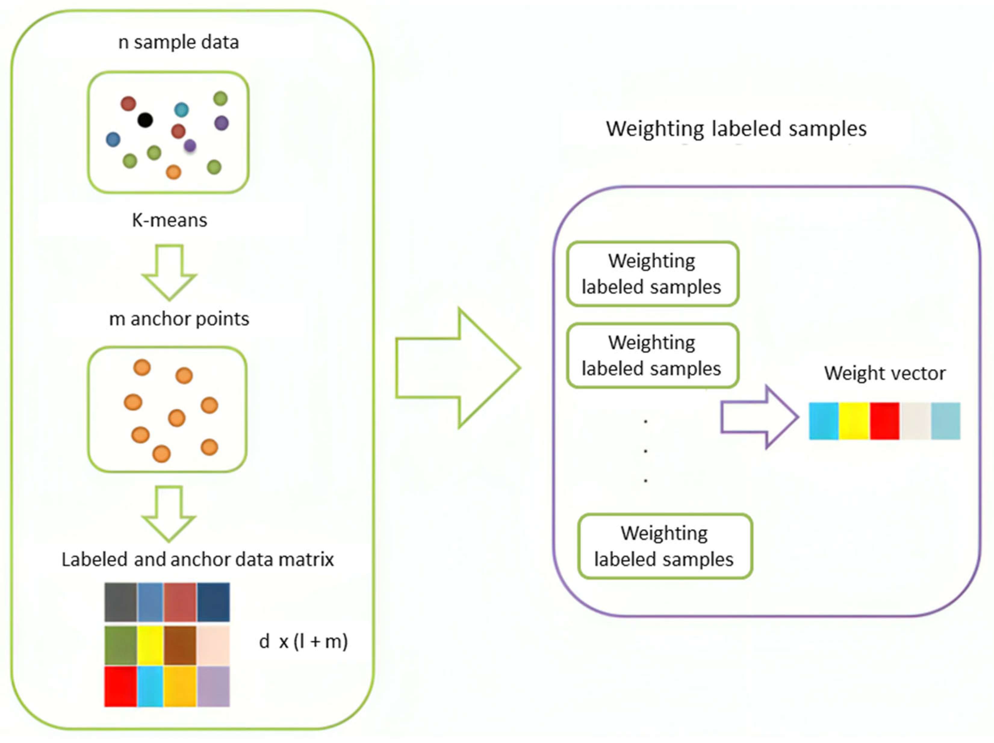
Figure 1. Modifying WS3C algorithm to make it adaptive for large datasets.
Information 15 00591 g001
Figure 2. Flowchart of the proposed method.
Information 15 00591 g002
Figure 4. Accuracy (%) of the proposed method with different ranges of values for p and t on the Norb dataset for unlabeled samples with o = 10.
Information 15 00591 g004
Figure 5. Accuracy (%) of the proposed method with different ranges of values for p and t on the Norb dataset for test samples with o = 10.
Information 15 00591 g005
Figure 6. Accuracy (%) of the proposed method with different values of μ and γ for the Norb dataset on the unlabeled data with o = 10 .
Information 15 00591 g006
Figure 7. Accuracy (%) of the proposed method with different values of μ and γ for the Norb database on the test data with o = 10 .
Information 15 00591 g007
Figure 8. Accuracy (%) of the proposed method with different values of μ and γ for the Covertype database on the unlabeled data with o = 30 .
Information 15 00591 g008
Figure 9. Accuracy (%) of the proposed method with different values of μ and γ for the CoverType database on the test data with o = 30 .
Information 15 00591 g009
Figure 10. Confusion Matrix, Precision, Recall, and F1 of the proposed method on the Norb dataset using o = 5.
Information 15 00591 g010
Figure 11. Confusion Matrix, Precision, Recall, and F1 of the proposed method on the CoverType dataset using o = 30.
Information 15 00591 g011
Table 1. Symbols used in this paper.
SymbolDescription
nNumber of samples
dDimensionality of samples
l Number of labeled samples
o Number of labeled samples per class
uNumber of unlabeled samples
m Number of anchor points
c Number of classes
p Percent of features
t Number of clusters
rNumber of iterations
μ ,   γ Balance parameters
X R d × n Data matrix
Y R n × c Binary label matrix
F R n × c Probability matrix of samples belonging to each label
Z R d × m Matrix of anchors
S R n × n Similarity matrix of data
A R ( m + l ) × ( m + l ) Probability matrix of sample belonging to same cluster
W ˜ R m × m Similarity matrix of anchors
B R n × m Similarity matrix of data with anchors
L R m × m Laplacian matrix of anchor graph
D ˜ R m × m Diagonal matrix
Q R d × c Projection matrix
P R ( m + l ) × ( m + l ) Affinity matrix of labels and anchors
b R c × 1 Bias vector
U R l × l Diagonal matrix for weights of labeled data
Table 2. Full names of articles referenced in this paper.
Method NameDescription
GSSLGraph-Based Semi-Supervise Learning
LGC [18]Local and Global Consistency
FME [11]Flexible Manifold Embedding
F-FME [13]Fast Flexible Manifold Embedding
R-FME [13]Reduced Flexible Manifold Embedding
WS3C [16]Weighted Sample-Based Semi-Supervised Classification
AGR [22]Anchor Graph Regularization
EAGR [23]Efficient Anchor Graph Regularization
MMLP [28]Minimax Label Propagation
MTC [29]Minimum Tree Cut
1NN1-Nearest Neighbor Classifier
LapRLS/L [30]Laplacian Regularized Least Square
Table 3. Algorithm of the proposed model.
Input:
-
n data points as X = X l , X u = x 1 , x 2 , x l , x l + 1 , x l + u that n = l + u ;
-
Binary label of data: Y = Y l , Y u ;
-
Parameters μ , γ , m , and t .
Output:
-
The prediction label matrix of training data F , the optimal projection matrix Q , and the optimal bias vector b are obtained.
-
Apply K-means clustering to data set X , with the resulting cluster centroids serving as anchor points.
-
Construct data matrix P = X l Z using the provided anchors and labeled samples.
-
Compute the matrix B R n × m by adopting the KNN graph construction method.Compute the weight of labeled samples using Equation (3).
-
Construct the proposed U matrix using Equation (9).
-
Compute A , Q , and b using Equations (6)–(8), respectively.
-
Compute F with Equation (4).
Table 4. Brief description of the adopted datasets.
DatasetNumber of SamplesNumber of FeaturesNumber of Features after PCA
Norb48,600921650
CoverType581,0125450
Table 5. Best parameters for the Norb dataset.
Norb
Type#Labeled Samples per Class#ClusterPercent of Features μ   V a l u e λ   V a l u e
Train102040% 10 12 10 6
Test102040% 10 1 10 6
Train832060% 10 1 10 6
Test82040% 10 1 10 6
Train532060% 10 1 10 6
Test532060% 10 1 10 6
Table 6. Best parameter for the CoverType dataset.
Cover Type
Type#Labeled Samples per Class#ClusterPercent of Features μ   V a l u e λ   V a l u e
Train707080% 10 3 10 2
Test707080% 10 6 10 3
Train507080% 10 3 10 3
Test507080% 10 3 10 2
Train307080% 10 3 10 3
Test307080% 10 3 10 2
Table 7. Average (%) and standard deviation of the accuracy over 20 trials for the proposed method and 8 other competing algorithms on the Norb database.
DatasetModel5 Labeled Samples8 Labeled Samples10 Labeled Samples
UnlabeledTestUnlabeledTestUnlabeledTest
Norb
N = 48,600
C = 5
M = 1000
AGR [22]41 ± 4.04
( 10 3 )
-48.28 ± 5.10
( 10 3 )
-52.34 ± 5.80
( 10 3 )
-
EAGR [23]44.79 ± 4.01
( 10 3 )
-52.10 ± 3.85
( 10 2 )
-55.79 ± 4.31
( 10 3 )
-
MMLP [28]41.61 ± 3.11-48.21 ± 3.98-52.86 ± 4.88-
MTC [29]38.22 ± 3.76-41.89 ± 3.23-45.61 ± 4.01-
1NN36.68 ± 2.0834.65 ± 2.3641.08 ± 2.3239.61 ± 2.0644.65 ± 2.0341.90 ± 1.80
LapRLS/L [30]45.23 ± 2.41
( 10 3 , 10 3 )
40.75 ± 3.75
( 10 3 , 10 3 )
49.76 ± 2.24
( 10 3 , 10 3 )
45.10 ± 3.02
( 10 3 , 10 3 )
51.9 ± 2.43
( 10 3 , 10 3 )
46.88 ± 2.89
( 10 3 , 10 3 )
F-FME [13]46.85 ± 2.54
( 10 0 , 10 15 )
41.74 ± 3.84
( 10 18 , 10 3 )
53.30 ± 3.11
( 10 0 , 10 18 )
46.36 ± 3.36
( 10 3 , 10 6 )
56.30 ± 3.25
( 10 0 , 10 18 )
47.95 ± 3.13
( 10 3 , 10 6 )
R-FME [13]50.09 ± 2.54
( 10 0 , 10 3 )
43.03 ± 3.58
( 10 0 , 10 6 )
56.40 ± 3.44
( 10 0 , 10 24 )
47.22 ± 3.21
( 10 21 , 10 6 )
59.95 ± 3.29
( 10 0 , 10 3 )
49.08 ± 2.69
( 10 9 , 10 6 )
Proposed Model53.02 ± 2.25
( 10 1 , 10 6 , 60 , 320 )
46.35 ± 2.34
( 10 1 , 10 6 , 60 , 320 )
58.59 ± 2.42
( 10 1 , 10 6 , 60 , 320 )
48.81 ± 1.58
( 10 1 , 10 6 , 40 , 20 )
60.86 ± 1.91
( 10 12 , 10 6 , 40 , 20 )
49.95 ± 2.03
( 10 1 , 10 6 , 40 , 20 )
Table 8. Average (%) and standard deviation of the accuracy over 20 trials for the proposed method and 8 other competing algorithms on the CoverType database.
DatasetModel30 Labeled Samples50 Labeled Samples70 Labeled Samples
UnlabeledTestUnlabeledTestUnlabeledTest
Covtype
N = 464,807
C = 7
M = 1000
AGR [22]44.00 ± 2.54 ( 10 2 ) -47.08 ± 2.73 ( 10 2 )-48.85 ± 2.30 ( 10 2 )-
EAGR [23]43.56 ± 2.4 ( 10 0 ) -46.35 ± 3.2 ( 10 0 ) -48.30 ± 2.69 ( 10 1 ) -
MMLP [28]40.58 ± 2.55-44.54 ± 2.79-46.90 ± 1.86-
MTC [29]40.50 ± 3.48-44.62 ± 3.39-48.21 ± 2.12-
1NN43.12 ± 2.2643.17 ± 2.2845.53 ± 1.1345.61 ± 1.1547.14 ± 1.6047.19 ± 1.64
LapRLS/L [30]44.48 ± 3.27 ( 10 3 , 10 6 ) 44.48 ± 3.30 ( 10 3 , 10 9 ) 48.86 ± 2.83 ( 10 6 , 10 9 ) 48.97 ± 2.83 ( 10 6 , 10 6 ) 50.50 ± 2.23 ( 10 6 , 10 9 ) 50.61 ± 2.25 ( 10 6 , 10 9 )
F-FME [13]48.27 ± 2.79 ( 10 0 , 10 6 ) 45.03 ± 6.62 ( 10 0 , 10 6 ) 48.86 ± 2.83 ( 10 0 , 10 6 ) 49.57 ± 2.98 ( 10 15 , 10 9 ) 51.94 ± 1.95 ( 10 0 , 10 6 ) 50.90 ± 2.08 ( 10 15 , 10 9 )
R-FME [13]47.70 ± 3.20 ( 10 15 , 10 3 ) 45.88 ± 3.87 ( 10 9 , 10 3 ) 49.54 ± 1.78 ( 10 24 , 10 6 ) 50.01 ± 3.14 ( 10 9 , 10 3 ) 51.89 ± 2.08 ( 10 9 , 10 3 ) 53.36 ± 2.74 ( 10 9 , 10 3 )
Proposed Model49.12 ± 2.07
( 10 3 , 10 3 , 70,80 )
48.86 ± 2.48
( 10 3 , 10 2 , 70,80 )
51.14 ± 2.20
( 10 3 , 10 3 , 70,80 )
51.52 ± 2.78
( 10 3 , 10 2 , 70,80 )
52.63 ± 1.65
( 10 3 , 10 2 , 70,80 )
53.97 ± 1.18
( 10 6 , 10 3 , 70,80 )
Disclaimer/Publisher’s Note: The statements, opinions and data contained in all publications are solely those of the individual author(s) and contributor(s) and not of MDPI and/or the editor(s). MDPI and/or the editor(s) disclaim responsibility for any injury to people or property resulting from any ideas, methods, instructions or products referred to in the content.