Article

Detection of Random Body Movements Using Clustering-Based Methods in Bioradar Systems

1
Instituto de Telecomunicações, Departamento de Eletrónica, Telecomunicações e Informática, Universidade de Aveiro, 3810-193 Aveiro, Portugal
2
Escola Superior de Tecnologia e Gestão de Águeda, 3750-127 Águeda, Portugal
3
AlmaScience Association—Pulp Research and Development for Smart and Sustainable Applications Madan Parque, Rua dos Inventores, 2825-182 Caparica, Portugal
4
IEETA, DETI, LASI, Universidade de Aveiro, 3810-193 Aveiro, Portugal
*
Author to whom correspondence should be addressed.
Information 2024, 15(10), 584; https://doi.org/10.3390/info15100584
Submission received: 19 August 2024 / Revised: 11 September 2024 / Accepted: 19 September 2024 / Published: 25 September 2024
(This article belongs to the Special Issue Signal Processing in Radio Systems)

Abstract

:
Bioradar systems, in general, refer to radar systems used for the detection of vital signs. These systems hold significant importance across various sectors, particularly in healthcare and surveillance, due to their capacity to provide contactless solutions for monitoring physiological functions. In these applications, the primary challenge lies in the presence of random body movements (BMs), which can significantly hinder the accurate detection of vital signs. To compensate the affected signal in a timely manner, portions of BM must be correctly identified. To address this challenge, this work proposes a solution based on the Density-Based Spatial Clustering of Applications with Noise (DBScan) algorithm to detect the occurrence of BM in radar signals. The main idea of this algorithm is to cluster the radar samples, aiming to differentiate between segments in which the subject is stable and segments in which the subject is moving. Using a dataset involving eight subjects, the proposed method successfully detects three types of body movements: chest movement, body rotation, and arm movement. The achieved results are promising, with F1 scores of 0.83, 0.73, and 0.8, respectively, for the detection of each specific movement type.

Graphical Abstract

1. Introduction

Bioradar is a technology that uses radio waves to monitor physiological signals such as heart rate and breathing [1]. This system has the potential to be used in healthcare and surveillance, allowing monitoring without any physical contact. This is advantageous in many situations where traditional methods cannot be applied [1]. As an example, in the context of monitoring elderly individuals, the non-contact nature of the system significantly enhances comfort. Additionally, when contrasted with camera-based systems [2], it provides the added advantage of ensuring privacy.
Bioradar systems rely on the Doppler effect to detect vital signs. They monitor the chest’s subtle movements during breathing and the finer heart pulsations. Given this, the presence of Body Movement (BM) can severely disrupt the signals being monitored. This disruption can lead to inaccuracies in readings, primarily due to the substantially larger amplitudes typically observed in BM related signals, in contrast to the signals generated exclusively due to the vital signs. In [3], the authors present a comprehensive review dedicated to the most used techniques for random body compensation, which include the usage of external modules in addition to the main radar system, signal processing techniques, and solutions based on phased-array antennas and beamforming techniques.
Recently, the most popular approaches relied on deep learning methods to separate the BM from stable respiratory motion [4,5,6]. In summary, while the proposed approach in [4] offers significant advantages in terms of interference removal and generalization, it also faces challenges related to noise sensitivity and interference modeling complexity. The Deep Neural Network (DNN)-based technique in [5] offers significant benefits in vital sign detection by canceling body movements without hardware changes. However, it also presents challenges due to the unpredictability of those movements and the reliance on high-quality training data. Additionally, the deep clustering approach in [6] shows substantial improvements in handling non-linear mixtures and enhancing accuracy; however, it presents challenges related to data dependency, implementation complexity, and overfitting risks.
However, most of the works reported in [3], as well as in [4,5,6], applied their proposed methodologies to offline data. This means that the data were previously collected and analyzed after the fact, allowing for the validation of their hypotheses without real-time constraints. In contrast, in a scenario of continuous acquisition involving online data—such as the real-time radar-based monitoring of human movements, where radar signals are continuously captured and analyzed—data are processed in real time, and the occurrence of BM must be correctly detected to ensure successful compensation and avoid unnecessary impact on signal quality [7]. An example of a system that does not use continuous acquisition would be radar-based motion detection systems used in controlled experiments, where radar data are recorded first and then analyzed offline to study specific movement patterns or to validate algorithms [8]. In [9], adaptive filters were used to compensate BM, and in this case, an accurate BM detector allows for the possibility of adjusting parameters during periods when the individual is perceived to be stable. In summary, while Radar-Beat presents significant advantages in contactless and robust heartbeat monitoring, it also faces challenges related to distance limitations, multi-person monitoring, and the need for further evaluation in clinical settings. The detection of sudden alterations can also be employed to detect falls or other movements of interest during vital signs acquisition [1].
In this sense, the literature also presents some options to detect BM. For instance, thresholding techniques take advantage of the magnitude disparity between BMs and chest motion during breathing to identify these movements [10]. However, defining a linear threshold for BM proves to be challenging due to variable factors, such as individual differences and changes in breathing patterns. ContinuousWavelet Transform (CWT)-based techniques have also been employed, capitalizing on the abrupt frequency changes caused by BM [11]. While CWT presents promise in detecting these movements, it may suffer from spectral leakage issues, potentially extending the perceived duration of movements. Autocorrelation methods exploit the stability of human breathing, showcasing effectiveness in identifying movement periods [12]. Nonetheless, it is also prone to fail due to natural respiratory alterations. Range-based techniques, particularly used in Impulse Radio Ultra Wide Band (IR-UWB) radar signals, offer distance estimation as a means to detect large body movements [13], but are constrained by the hardware requirements of IR-UWB technology. Furthermore, in [10,11,12,13], quantitative evaluations of their effectiveness in detecting BM remain limited, posing a challenge for practical implementation.
A notable contribution in this domain is the work presented in [14]. This study explores the use of Continuous-Wave (CW) radar sensors for distinguishing Doppler signals generated by human gestures based on a Single Input Multiple Output (SIMO) front end and a blind motion-separation algorithm.
In this work, we propose a novel method based on a clustering approach to identify BM occurrences. Initially, a preliminary study was conducted to compare the performance of the K-means algorithm with Density-Based Spatial Clustering of Applications with Noise (DBSCAN) using data from four subjects. Based on this comparison, DBSCAN was selected as the more effective approach. DBSCAN was applied to baseband radar samples from a large dataset comprising eight subjects. These subjects moved purposefully in a controlled scenario following a specific protocol. To enhance accuracy, noise segmentation was further explored as a means to reduce false BM detections. Finally, we propose a generalization of DBSCAN parameters to eliminate prior knowledge dependencies.
The article is organized as follows: Section 2 describes the dataset and the experimental setup, and Section 3 analyzes the differences between two traditional clustering methods, DBSCAN and K-means, followed by a thorough discussion of the proposed method in Section 4. Section 5 suggests a method alteration to simplify its implementation and generalize its suitability to new signals. Finally, Section 6 presents the conclusions, pointing out potential directions for future research.

2. Dataset and Setup Description

This chapter outlines the dataset acquisition and experimental setup. Two datasets were acquired: the first, containing data from two subjects, will be examined in Section 3 to compare the performance of K-means and DBSCAN algorithms in detecting BM within the context of monitoring vital signs. The second dataset, consisting of eight subjects, will be analyzed in Section 4 using the optimal model determined in the previous section. In both datasets, vital signs were recorded with participants seated to reduce involuntary movements and minimize unwanted activity. Subjects’ characteristics are detailed in Table 1. The study was approved by the Ethics and Deontology Committee of the University of Aveiro, Portugal (No. 10-CED/2023), following the Declaration of Helsinki, with all participants providing informed consent. As the goal is to develop an algorithm for BM detection during the monitoring of vital signs, the data-collection protocol incorporated alternating periods of purposeful movement and stable recording phases. To enhance reproducibility and control variability, a well-defined movement protocol was implemented, reducing the influence of individual differences in movement execution [12].
As this paper intends to propose an algorithm that detects BM in the context of the detection of vital signs, the implemented data-collection protocol encompassed interspersed periods of purposeful motion and periods of vital signs captured while the subject was stable. In the scope of reproducibility and variability control, it is important to define a clear protocol of movements and thus restrict the impact of inter-subject variability in the execution of movements [12].
The signal acquisition lasted 12 min in total for each subject, and it was composed of seven different moments: stable breathing→movement 1→stable breathing→movement 2→stable breathing→movement 3→stable breathing. The movements happened at approximately minutes 2, 6, and 10 after the beginning of the experiment. Following this, the recorded signals were partitioned into three segments, each spanning 4 min, for individual processing. Each segment contains a portion of stable breathing and a portion of movement. The movements are illustrated in Figure 1 and can be described as follows:
  • Movement 1—Moving the chest back and forth (approximately 10 cm);
  • Movement 2—Rotating the body to each side (approximately 30–45 degrees);
  • Movement 3—Moving each arm above the head, one at a time.
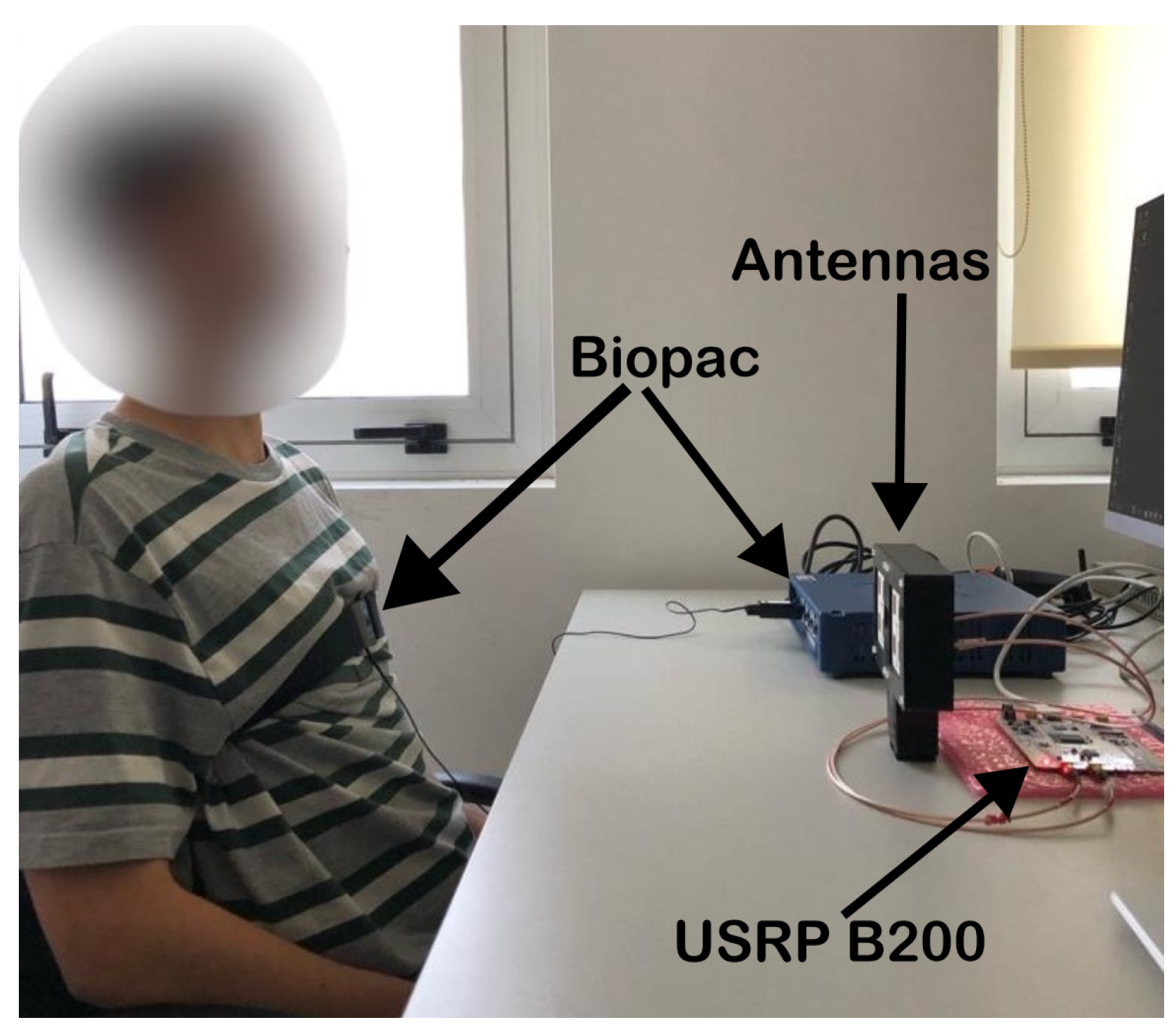
The experiment was conducted in controlled conditions, with a wall behind the person and no other objects in the radar surroundings, as depicted in Figure 2. It was also ensured that no external movement happened within the illuminated area of the antenna beam apart from the person’s Respiratory Movement (RM) and BM. The distance between the subject’s chest and the radar was about 50 cm.
The system used for the data acquisition consisted of a CW radar using an Software Defined Radio (SDR) board (the USRP B200), two 2 × 2 antennas working at 5.8 GHz and a computer used to collect the data using GNU Radio software (v3.10.10.0). The data were then processed using MATLAB R2021b. The signals were originally collected at 100 kHz but then downsampled to 20 Hz. This sample rate was chosen to optimize the DBScan algorithm computational time without compromising the representativeness of the signal, as fewer samples require less computational effort for clustering. Also, it has been proven that human motion has all frequency components below 20 Hz [15], including the breathing rate, which can achieve a maximum rate of 0.4 Hz [16]. Given this, the chosen sampling rate is more than enough to capture all motion required.

3. Clustering Methods

One of the most used applications of Machine Learning (ML) is clustering. In a clustering algorithm, a set of data points is classified into groups based on their similarities; data points that have similar traits and/or properties are placed in the same group; otherwise, they are grouped into different groups. Clustering is an unsupervised learning method. In the field of data science, clustering analysis is used to extract valuable information from the data, as it categorizes the data into different clusters. This section examines K-means clustering and DBSCAN.

3.1. K-Means Clustering

The K-means clustering method is a straightforward and original type of unsupervised machine learning clustering.
In order to apply conventional K-means clustering in a data set, the first step is to choose a random number of cluster centroids ( k ) , which are data points that represent cluster centers. In order to determine the k value, the collected data is typically viewed, and any dissimilar groups are sought. Based on the distance between each data point and each cluster centroid, the point is classified into the closest cluster. After classifying every point, the centroids are recalculated by doing the mean of all the vectors in each defined group. The process is complete when the centroids remain in the same spot after a set number of iterations.
The K-means clustering approach is fast and easily scalable, as it only needs to compute the distance between the data points and the group centroids. This method has some disadvantages, namely that the initial centroids chosen have a significant impact. This method starts with a random choice of centroids and can lead to different clustering results for different runs, producing results that are not repeatable with the same algorithm. This model is also sensitive to cluster size, shape, and density [17].

3.2. Density-Based Spatial Clustering of Applications with Noise

DBSCAN is also an unsupervised machine learning technique that can identify clusters of varying size and shape [18].
This method starts with a random data point from the data set, where its neighborhood is retrieved using the distance ε as the maximum range from the starting point. Moreover, it is defined as a minimum number of samples so that clustering begins only at the current point if the neighborhood has the same number of points; otherwise, the point will be considered noise. The process of including the points in the ε range from the defined point is repeated for all new points that have been added to the group, and this procedure is repeated until all the points in the ε distance of the neighborhood have been labeled. In the next step, a point outside the ones already selected is selected to detect noise or a cluster. This is carried out until all data points are computed, resulting in each point being marked as a cluster member or noise.
DBSCAN does not require a preset number of clusters like the K-means clustering method. It recognizes outlier values as noise and can identify clusters of any size and shape. However, DBSCAN does not perform as well as other methods when clusters have a variation in density or when there are a large number of data because its neighborhood identification parameters ( ε and minimum number of samples) change when the density of the clusters varies. If the clusters are not well separated, this method can also have some trouble distinguishing between them.

3.3. Data Description, Visualization and Statistical Analysis

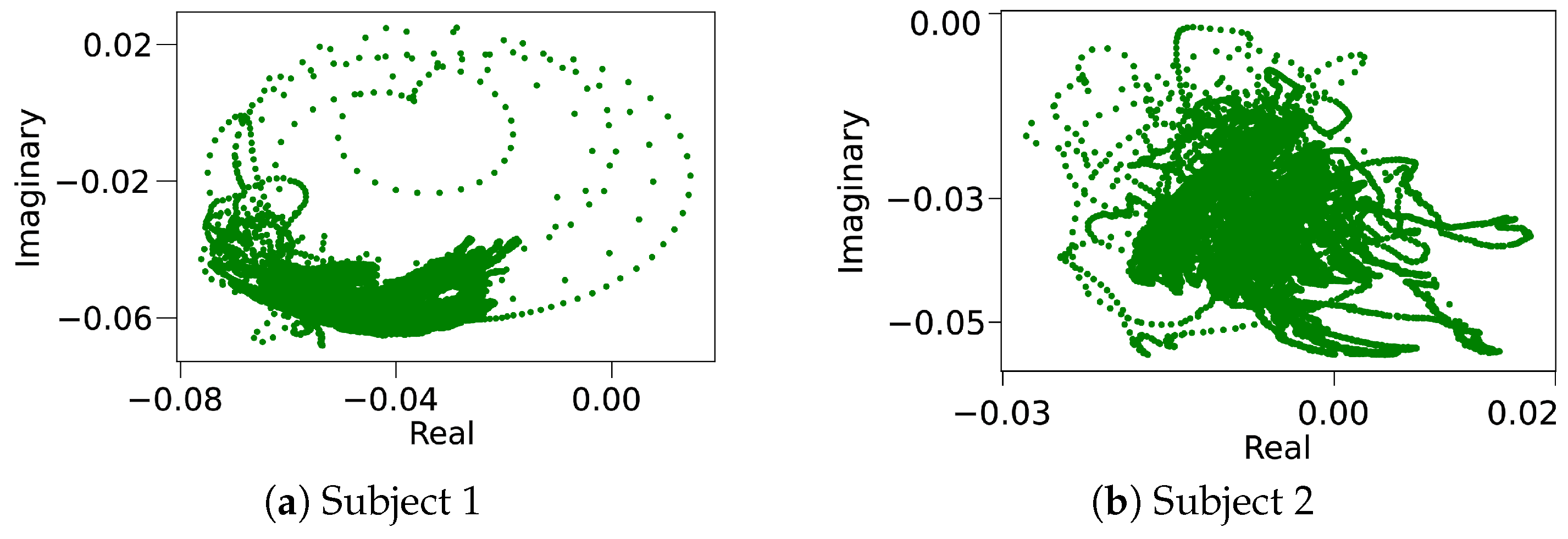
For the purpose of achieving this work’s goal, which is to remove involuntary motions from the subjects’ signals, Figure 3 shows the signal directly acquired by the Bio-Radar for each subject [8], resulting in dataset 1 as depicted in Table 1.
Figure 3 demonstrates that the movements that need to be eliminated are quite noticeable. This is because the largest spot of dots corresponds to small movements of the rib cage caused by the heart beating and by breathing [8]. In order to detect these small variations, it is required that the noise be as low as possible.

3.4. Implementation

As explained earlier, two models (DBSCAN and K-means) were used to remove the involuntary movements of the subjects when they are performing the test.

3.4.1. K-Means

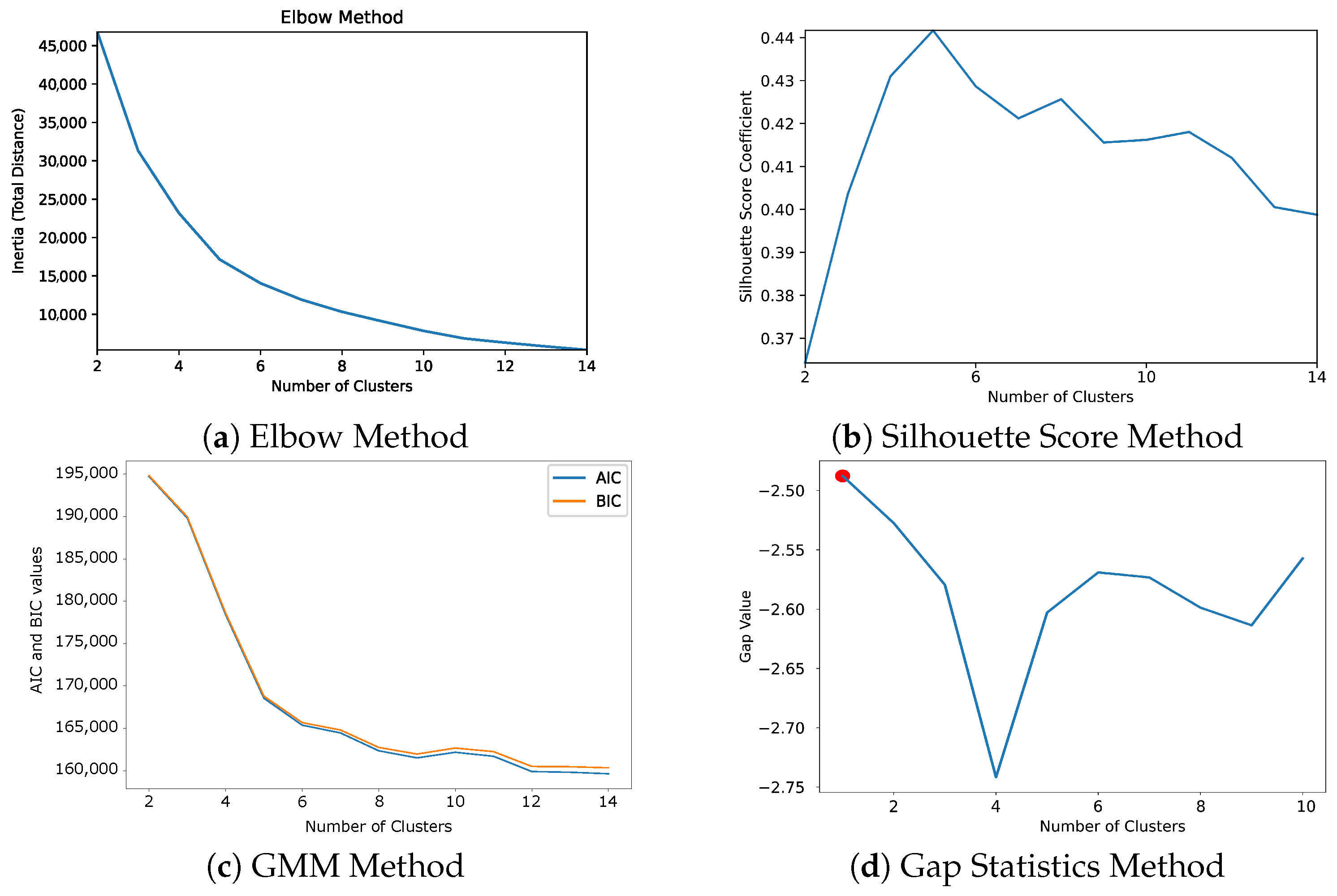
When using K-means the most relevant parameter is k, as mentioned earlier. Thus, there are several methods responsible for optimizing this parameter among them: the Elbow Method [19], the Silhouette Score Method [20], the Gaussian Mixture Modelling (GMM) Method [21], and the Gap Statistics Method [22]. Figure 4 shows the four methods implemented for one subject as an example.
Considering the problem in study, this model is suboptimal. By viewing Figure 4, it is possible to identify that there is no standard for the value of k. This means that the models used have some difficulty finding an optimal k parameter.
So, for the purpose of comparison with the model that will be discussed later in this paper, we assume that the optimal value of k is given to us by the Silhouette Score Method depicted in Table 2.
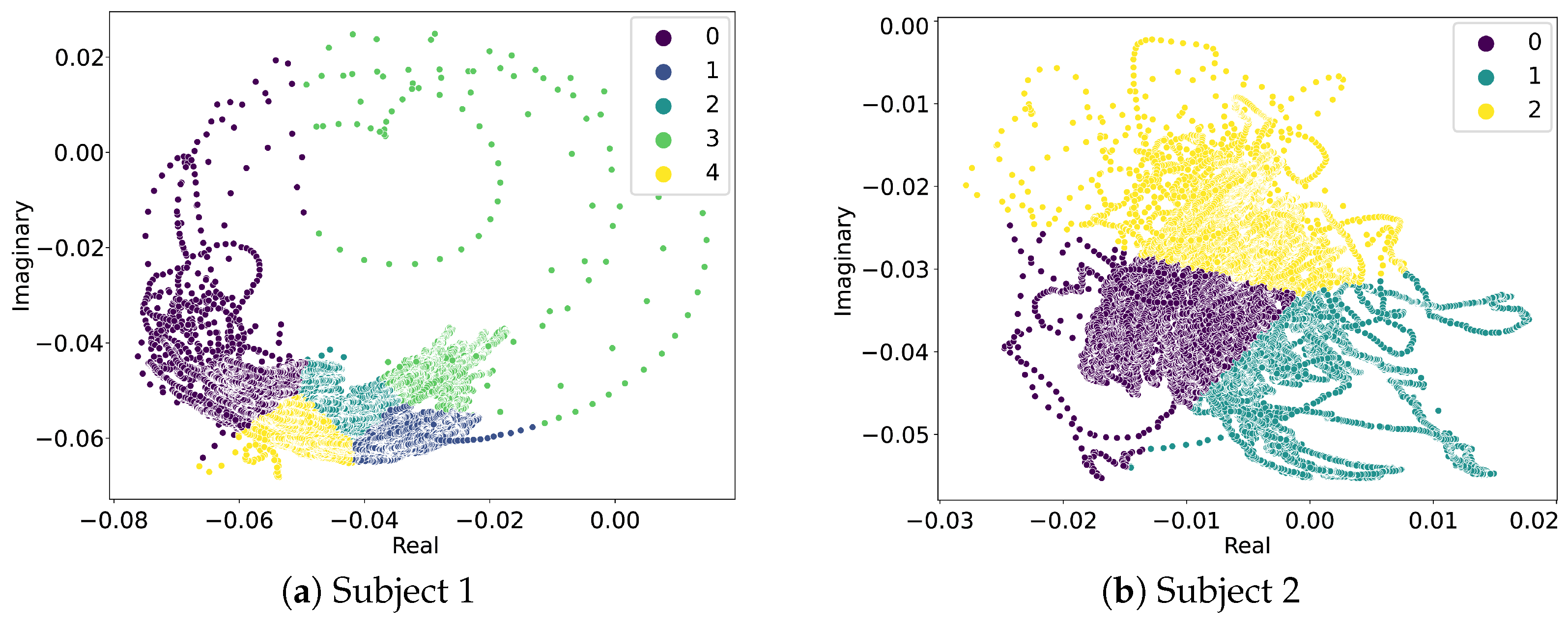
Figure 5 shows the final representation of the results obtained by implementing the K-means algorithm.
Even though the results in Table 2 demonstrate the effectiveness of the K-means algorithm, by looking at Figure 5, we can conclude that the removal of involuntary movements did not occur as expected.

3.4.2. DBSCAN

In view of the malfunction of the algorithm demonstrated earlier, another algorithm based on DBSCAN was implemented. In this type of scenario, when using DBSCAN, the most relevant parameters to be calculated are the ϵ and the minimum samples. To do that, we use one of the most used methods to find the optimal epsilon, which is the nearest neighbor distance. This model is a supervised machine learning clustering algorithm that clusters new data points based on their distance from other “known” data points. In Figure 6, the corresponding graphs for each subject are shown [23].
As you can see in Figure 6, the “elbow region” gives the optimal epsilon values to be simulated. Therefore, this parameter was simulated in the range [0.08–0.15] for all subjects.
It is also necessary to find the optimal values for the minimum number of samples. This parameter can be obtained using the expression (1) [24]
M i n s a m p l e s = 20 × ( 2 × N u m b e r f e a t u r e s )
Therefore, in the case being studied in this paper, and given that the number of features is equal to 2 (real and imaginary), the value of the minimum samples are varied between 75 and 85.
As a result of simulations running for the previously discriminated values, the optimal values for each parameter per subject are shown in Table 3.
Figure 7 shows the final representation of the results obtained by implementing the DBSCAN algorithm.
As can be seen in Figure 7, in all cases, it was possible to remove the subjects’ involuntary movements effectively, and this corroborates the values present in Table 3. It should be noted that the decision of which cluster is chosen is the one with the highest number of samples. An outlier (involuntary move) is considered when the label equals −1.

3.5. K-Means vs. DBScan

Since the goal of this work is to remove from the signal acquired by the Bio-Radar, the involuntary movements of the subjects who are performing the test, by viewing Figure 5 and Figure 7, it is possible to see that DBSCAN presents better results compared to K-means. It is clear that in general terms, the silhouette value is better for K-means, but it cannot accomplish the final goal, so we can say that the highest value is not always the most significant, which is the case in this work.

4. Methodology Description

After the radar signal acquisition, signals were downconverted to baseband and downsampled, as previously described in Section 2. Radio frequency front-ends are often composed of quadrature receivers; therefore, the baseband signals are processed as complex signals. Figure 8a shows a blue arc projected in the complex plane, which represents the respiratory function under ideal conditions, i.e., without any BM. Depending on the exact motion, the occurrence of BM will affect the shape of the arc, since it generates a signal with an amplitude higher than the vital signs. Figure 8a represents the appearance of the complex plane, while the body is moving forward and backward in relation to the radar, marked with an orange dashed line. The corresponding time domain signal is shown in Figure 8b.
According to Figure 8, one can anticipate that both components can be easily separated using clustering methods due to their amplitude differences. The proposed algorithm is depicted in the block diagram in Figure 9. The main idea of the algorithm is that the DBScan algorithm should be able to cluster the signal retrieved from the radar into two groups: segments contaminated with BM and segments with RM only.
The rest of this section will be used to better describe the blocks presented in Figure 9. For better visualization and easier signal analysis, complex radar signals are presented without the DC offsets component, removed using the Circle-Fitting method [25,26]. Time domain signals that will be shown were obtained through Arctangent Demodulation [27].

4.1. DBScan

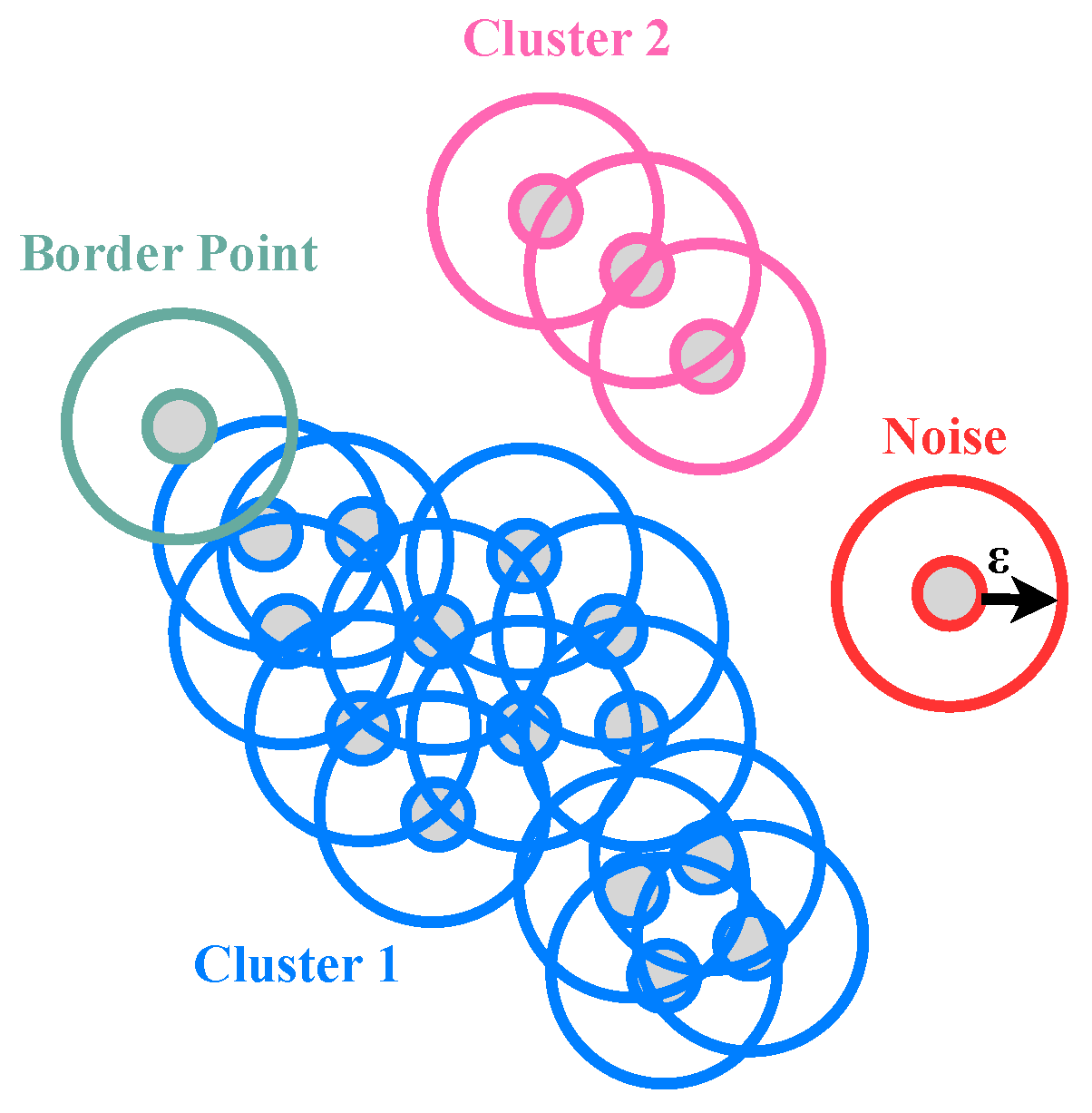
As explained earlier in this document, when DBSCAN is compared with K-means, DBSCAN is an unsupervised machine learning technique that can identify clusters of varying sizes and shapes [28]. Figure 10 depicts the method’s working principle. This method starts by considering a random data point from the dataset as the Starting Point, and its neighborhood is retrieved using the distance ε as the maximum range. Each point within the ε range is evaluated and labeled until all the points of the neighborhood have been labeled. The variable Minimum Number of Points (MinPts) is defined as the minimum number of points necessary to create a cluster; otherwise, those points are considered as noise. Border points are an exception, as they do not need to have MinPts in their total ε range as long as they are in the ε neighborhood of other cluster points.
Therefore, the two main parameters of the DBSCAN algorithm are MinPts and ε , and choosing the correct value for these variables is the key to guaranteeing the performance of this clustering method [29].
The selection and fine-tuning of these parameters have been the subject of extensive investigation in the literature. When it comes to the choice of MinPts, the original DBScan article [28] suggests that for a dataset with two dimensions, which is the case of this study (real and imaginary), the value of MinPts should be 4. However, more recent studies show that the optimal value for this parameter is highly dependent on the type of data and the amount of noise in a dataset [29]. Moreover, for sequences with a large amount of data and/or a lot of noise, it is usually recommended for this parameter to be set to a higher value than 4.
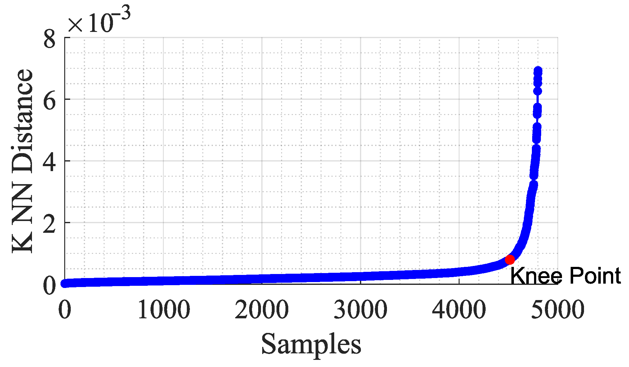
When it comes to the parameter ε , it is usually selected based on the vectorial distances between the samples in the dataset [30]. For the case of our proposed method, the average of the distances from each point to its k nearest neighbors (KNNs) ( k = M i n P t s 1 ) is calculated and then plotted in ascending order. In Figure 11, there is usually a “knee” point. This knee point marks a significant transition in the plot, i.e., it signifies the shift from a region of sparse data distribution to a region of denser data concentration. In other words, it represents the boundary between areas where points are scattered and areas where they are more tightly packed, thus corresponding to the optimal ε . Choosing the ε value at this point allows the capturing of meaningful clusters while also filtering out noisy data points.
As previously discussed, the usual calculation of ε requires the knowledge of the MinPts parameter, which in itself is highly dependent on the knowledge of the data to be clustered. To overcome this aspect, for each sequence in the dataset, results were inspected for different values of MinPts within the range of 2 to 100 points. This upper boundary was chosen considering that a normal breathing period takes an average of 5 s and the signals were sampled at 20 Hz. Thus, the algorithm requires only one breath to generate a cluster. For each value of MinPts, the ε was calculated using the KNN method [30]. In this method, it is necessary to choose the “knee” point, and for this purpose, the MATLAB function Knee Point proposed in [31] was used.
In order to evaluate the accuracy of the DBScan algorithm in finding BM sequences, the results of this step were compared to the ones obtained by identifying BM sequences manually by visual inspection. The quality of the results was assessed using the F1 score (originally named the Dice coefficient [32]), given by Equation (2), which takes into account the Precision and the Recall given by Equations (3) and (4), respectively.
F 1 Score = 2 × Precision × Recall Precision + Recall
Precision = T P T P + F P
Recall = T P T P + F N
In this context, we define these metrics as
  • True Positive (TP): Correct detection of BM;
  • False Positive (FP): False detection of BM;
  • True Negative (TN): Correct detection of RM;
  • False Negative (FN): False detection of RM;
The ideal values for Precision, Recall, and F1 Score are 1, which would mean that all positives (in this case BM) are detected, while no false positives occur. For this context, we will consider that precision and recall are equally important, but this might not always be the case [33].
Table 4 shows the results, considering the MinPts value that provided the best F1 score for a specific movement. The movements used to perform this test were randomly selected. It can be seen that the optimal value of MinPts varies a lot depending on the data in question.
The variation in the optimal parameters can be justified by the individual variability in the breathing motion. For instance, breaths that are deeper than usual in a sequence can often be classified as BM. This happens because these deeper breaths generate points in the polar plot that are further away from the densest areas in the RM cluster. Given that DBSCAN is based on the density of the points, less dense areas are usually considered as noise.
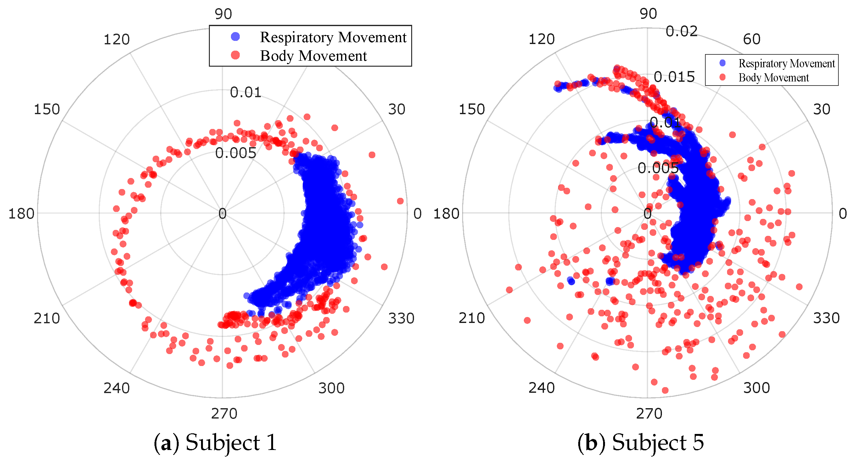
This effect is particularly noticeable in the polar plot in Figure 12b and Figure 13b, where a deeper breath generates a deviation from the original arc, which could be perceived as noise. Figure 13 presents the polar plot of DBSCAN results, where the angular values represent the phase information captured by radar signals. In these plots, the angular distribution differentiates between respiratory movement (blue) and body movement (red). Respiratory movements tend to cluster within specific angular regions due to their consistent and periodic nature. In contrast, body movements show greater variability and occupy a broader angular range. The concentration of blue points in certain angular regions reflects the stability and periodicity of the breathing phase. The more scattered red points indicate sporadic and less periodic body movements. This distinction is critical in the experiment. It demonstrates how the DBSCAN algorithm can effectively cluster and separate these two types of movement based on their phase information. This allows for better signal processing and compensation. In this case, specifically, the optimal MinPts was set to 3, which is in the lowest part of the range. Increasing the value of ε or the value of MinPts would result in the inclusion of these points in the RM cluster, but in turn would generate more FP.
When it comes to FN, these can also be seen in both of the examples mentioned in Figure 12. More particularly, in Figure 12a, it is clearly noticeable that the beginning and end of the movement portions are not considered as BM. On the other hand, in the Subject 5 example in Figure 13b, some portions inside the movement window are incorrectly labeled as RM, too.

4.2. Noise Segmentation

The previous section highlighted the two major problems related to the DBSCAN approach used for BM detection:
  • Deeper breaths can generate FP (i.e., incorrectly labeling sequences as BM).
  • FN can be generated by certain types of movement that generate random points spread over the real/imaginary axis and by the breathing itself, even when a person is not moving.
Given the problems previously mentioned, for the BM detection purpose, one will only contemplate sequences where movement lasts at least 1 s. Thus, a sliding window can be applied to better identify the exact occurrence of BM.
Applying a sliding window technique over the DBSCAN result will allow the algorithm to “ignore” FP generated by deeper breaths, given that even in these types of breaths most points are considered RM. This approach will also allow the algorithm to gather sequences of movement that are briefly separated by RM, reducing the amount of FN. Therefore, this last layer of the movement detection algorithm consists of the following steps (see Figure 9):
  • Windowing: The binary data obtained from the DBSCAN algorithm (0 = RM, and 1 = BM) are divided into overlapping windows of fixed size WindowSize and an overlap OverlapPercentage.
  • Ones percentage calculation: Since, even when there is motion, some points are still often labeled in the RM cluster, the percentage of one-valued points is calculated within each window.
  • Threshold-Based Decision: A decision criterion is established based on a threshold parameter, denoted as minOnesPercentage. If the calculated “ones” percentage within a window surpasses this threshold, the window is labeled as a BM segment; otherwise, it is labeled as RM segment.
  • BM Segment Stitching: The windows identified as BM segments are combined to form larger regions of BM. This step is pretty simple, and it just takes the end of one BM section and the start of the following one and verifies the distance (in samples) between both. If the distance is lower than a variable: maxStitchDistance, then the two segments are grouped into a contiguous one.
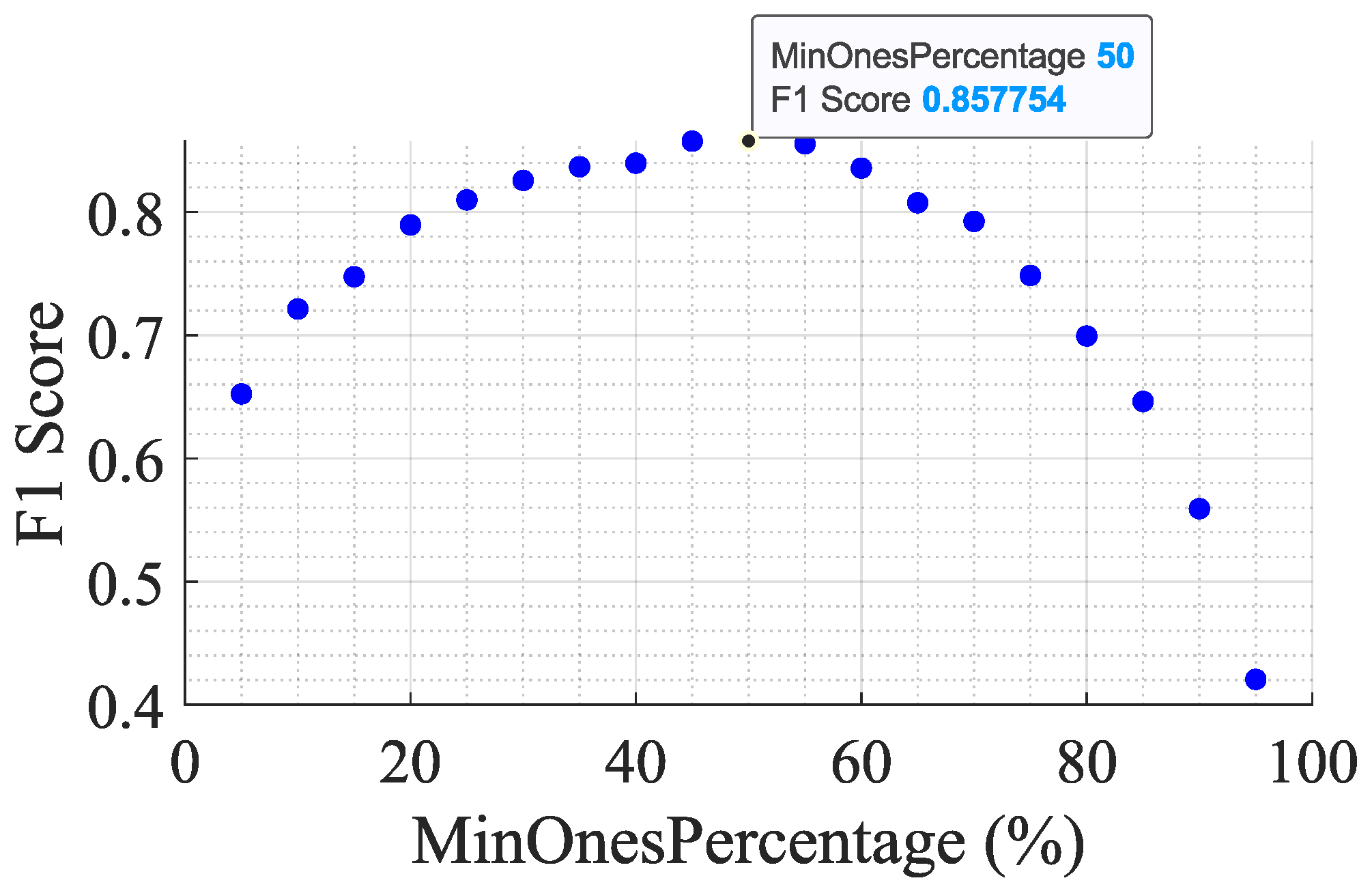
Given that the purpose is to detect movement sections whose duration is at least 1 s, WindowSize and maxStitchDistance were set to 20 samples considering the sampling frequency of 20 Hz, with an OverlapPercentage of 80%. When it comes to minOnesPercentage, percentages from 5 to 100% were tested. Figure 14 shows the F1 score results, where the best one was achieved with a minOnesPercentage of 50%.
After the processing steps, the results were once again assessed using the F1 score metric for the same eight motion signals considered in Table 4. As can be seen in Table 5, the overall F1 scores improved significantly in this step, with an average F1 score of 0.86, an average precision of 0.87, and an average recall of 0.85.
When comparing the results of Subjects 1 and 5 before and after the Noise Segmentation, the improvements are clear. For Subject 1’s sequence (Figure 15a and Figure 16a), most parts of BM are now labeled correctly. The beginning of the movement portion is still considered as RM, but only by a fraction less than a second. When it comes to FP, there is only a slight section after the BM ends that is incorrectly labeled.
For Subject 5’s sequence (Figure 15b and Figure 16b), most of the deeper breaths that caused FP are now included in the RM cluster, resulting in a precision of 0.90.

5. DBScan Parameter Generalization

The earlier approach faced a significant challenge due to the need for optimizing two variables: MinPts and ε . Achieving optimal results while optimizing MinPts was contingent on understanding the noise within the dataset, which could be limiting if such insights are unavailable a priori.
The initial results in Table 4 show that the clustering algorithm alone is not enough to correctly depict sequences with movement. This happens because BM generates points spread along the real/imaginary axis, even superimposed with the boundaries of the RM cluster. This hampers the separation of BM segments from the RM signal, which in turn leads to the necessity of including the noise segmentation block.
After including the noise segmentation block, it is noticeable that these effects become less prominent, increasing the overall F1 Score, as Table 5 shows. However, the fact that the “optimal” values for MinPts are calculated with the knowledge of the temporal section where BM happens artificially improves the F1 Score. This means that using this approach would be impossible in a real-life scenario.
To address this, and following the recommendation in [28], a constant MinPts value of 4 was adopted. Changing the approach to the choice of MinPts by setting it to the recommended value of 4 allows the algorithm to work without any previous knowledge about the noise in the data. With this value of MinPts, we used the method discussed previously to define a value for ε for each sequence. Furthermore, using this value, we did an assessment of all the movements from all the subjects, and the average results for each movement type are presented in Table 6.
For this approach, the results were worse than the averages presented in Table 5, but still showed that most BM points are still correctly depicted while not showing too many FPs. It was noted that for movement type number 2, the results were slightly worse, which might be related to the characteristics of the movement itself.

6. Conclusions

In this work, we developed a method based on DBSCAN to detect BM during the acquisition of vital signs in bioradar systems. The proposed approach was tested on three distinct types of body movements—chest movement, body rotation, and arm movement—with corresponding F1 scores of 0.83, 0.73, and 0.80, respectively. These results demonstrate the effectiveness of the DBSCAN-based clustering approach in distinguishing BM from RM across various movement types. Furthermore, the parameter optimization process enabled the algorithm to generalize across different subjects with minimal prior knowledge of the dataset. Although the results are promising, further validation is needed in real-world settings with natural, unpredictable body motions. Future work will focus on automating the selection of the ε parameter and evaluating the algorithm’s performance in extended scenarios, such as long-term monitoring applications.

Author Contributions

Conceptualization, A.R.; Methodology, A.R.; Software, A.R., F.S., B.S., D.A. and C.G.; Formal analysis, A.R. and S.B.; Investigation, A.R., B.S., D.A., C.G. and S.B.; Data curation, A.R.; Writing—original draft, A.R., F.S. and B.S.; Writing—review & editing, D.A., C.G., S.B. and P.P.; Visualization, A.R.; Supervision, D.A., C.G., S.B. and P.P.; Project administration, P.P. All authors have read and agreed to the published version of the manuscript.

Funding

This work is funded by the Fundação para a Ciência e Tecnologia (FCT) through Fundo Social Europeu (FSE) and by Programa Operacional Regional do Centro under the PhD grant 2023.00385.BDANA and 2024.00376.BD. S.B. is funded by (https://doi.org/10.54499/DL57/2016/CP1482/CT0096) national funds, European Regional Development Fund, FSE through COMPETE2020, through FCT, in the scope of the framework contract foreseen in the numbers 4, 5, and 6 of article 23, of the Decree-Law 57/2016, of August 29, changed by Law 57/2017, of 19 July. It was also funded by FCT/Ministério da Ciência, Tecnologia e Ensino Superior (MCTES) through national funds and, when applicable, co-funded by the European Union (EU) fund under the project 2022.05005.PTDC and the projects UIDB/00127/2020 (IEETA/UA) and UIDB/50008/2020-UIDP/50008/2020 (IT).

Institutional Review Board Statement

The study was approved by the Ethics and Deontology Committee of the University of Aveiro, Portugal (No. 29-CED/2021). The implemented procedure was in line with the Declaration of Helsinki.

Informed Consent Statement

Informed consent was obtained from all subjects involved in the study. Written informed consent has been obtained from the patient(s) to publish this paper.

Data Availability Statement

The datasets presented in this article are not readily available because the data are part of an ongoing study.

Conflicts of Interest

Author Carolina Gouveia was employed by the company AlmaScience Association-Pulp Research and Development for Smart and Sustainable Applications Madan Parque. The remaining authors declare that the research was conducted in the absence of any commercial or financial relationships that could be construed as a potential conflict of interest.

References

  1. Islam, S.M.M. Radar-based remote physiological sensing: Progress, challenges, and opportunities. Front. Physiol. 2022, 13, 955208. [Google Scholar] [CrossRef] [PubMed]
  2. Gu, C.; Wang, G.; Li, Y.; Inoue, T.; Li, C. A Hybrid Radar-Camera Sensing System with Phase Compensation for Random Body Movement Cancellation in Doppler Vital Sign Detection. IEEE Trans. Microw. Theory Tech. 2013, 61, 4678–4688. [Google Scholar] [CrossRef]
  3. Gouveia, C.; Vieira, J.; Pinho, P. A review on methods for random motion detection and compensation in bio-radar systems. Sensors 2019, 19, 604. [Google Scholar] [CrossRef]
  4. Czerkawski, M.; Ilioudis, C.; Clemente, C.; Michie, C.; Andonovic, I.; Tachtatzis, C. Interference Motion Removal for Doppler Radar Vital Sign Detection Using Variational Encoder-Decoder Neural Network. In Proceedings of the 2021 IEEE Radar Conference (RadarConf21), Atlanta, GA, USA, 7–14 May 2021; pp. 1–6. [Google Scholar] [CrossRef]
  5. Gu, C.; Wang, J.; Lien, J. Deep Neural Network based Body Movement Cancellation for Doppler Radar Vital Sign Detection. In Proceedings of the 2019 IEEE MTT-S International Wireless Symposium (IWS), Guangzhou, China, 19–22 May 2019; pp. 1–3. [Google Scholar] [CrossRef]
  6. Ye, C.; Gui, G.; Ohtsuki, T. Deep Clustering with LSTM for Vital Signs Separation in Contact-free Heart Rate Estimation. In Proceedings of the ICC 2020-2020 IEEE International Conference on Communications (ICC), Dublin, Ireland, 7–11 June 2020; pp. 1–6. [Google Scholar] [CrossRef]
  7. Woo, S. Online continual learning for human activity recognition. Pervasive Mob. Comput. 2023, 93, 101817. [Google Scholar] [CrossRef]
  8. Gouveia, C.; Albuquerque, D.; Vieira, J.; Pinho, P. Dynamic Digital Signal Processing Algorithm for Vital Signs Extraction in Continuous-Wave Radars. Remote Sens. 2021, 13, 4079. [Google Scholar] [CrossRef]
  9. Zhang, H.; Jian, P.; Yao, Y.; Liu, C.; Wang, P.; Chen, X.; Du, L.; Zhuang, C.; Fang, Z. Radar-Beat: Contactless beat-by-beat heart rate monitoring for life scenes. Biomed. Signal Process. Control 2023, 86, 105360. [Google Scholar] [CrossRef]
  10. Hu, W.; Lie, D.; Kakade, M.U.; Ichapurapu, R.; Mane, S.; Lopez, J.; Li, Y.; Li, C.; Banister, R.; Dentino, A.; et al. An intelligent non-contact wireless monitoring system for vital signs and motion detection. In Proceedings of the 2010 International Conference on System Science and Engineering, Taipei, Taiwan, 1–3 July 2010; pp. 190–194. [Google Scholar] [CrossRef]
  11. Mercuri, M.; Lorato, I.R.; Liu, Y.H.; Wieringa, F.; Hoof, C.V.; Torfs, T. Vital-sign monitoring and spatial tracking of multiple people using a contactless radar-based sensor. Nat. Electron. 2019, 2, 252–262. [Google Scholar] [CrossRef]
  12. Khan, F.; Cho, S.H. A detailed algorithm for vital sign monitoring of a stationary/non-stationary human through IR-UWB radar. Sensors 2017, 17, 290. [Google Scholar] [CrossRef] [PubMed]
  13. Baldi, M.; Appignani, F.; Zanaj, B.; Chiaraluce, F. Body movement compensation in UWB radars for respiration monitoring. In Proceedings of the 2012 IEEE First AESS European Conference on Satellite Telecommunications (ESTEL), Rome, Italy, 2–5 October 2012; pp. 1–6. [Google Scholar]
  14. Gu, Z.; Wang, J.; Shen, F.; Xu, K.; Ye, D.; Huangfu, J.; Li, C.; Ran, L. Blind Separation of Doppler Human Gesture Signals Based on Continuous-Wave Radar Sensors. IEEE Trans. Instrum. Meas. 2019, 68, 2659–2661. [Google Scholar] [CrossRef]
  15. Khusainov, R.; Azzi, D.; Achumba, I.E.; Bersch, S.D. Real-time human ambulation, activity, and physiological monitoring: Taxonomy of issues, techniques, applications, challenges and limitations. Sensors 2013, 13, 12852–12902. [Google Scholar] [CrossRef] [PubMed]
  16. Nicolò, A.; Massaroni, C.; Schena, E.; Sacchetti, M. The importance of respiratory rate monitoring: From healthcare to sport and exercise. Sensors 2020, 20, 6396. [Google Scholar] [CrossRef] [PubMed]
  17. Jain, A.; Duin, R.; Mao, J. Statistical pattern recognition: A review. IEEE Trans. Pattern Anal. Mach. Intell. 2000, 22, 4–37. [Google Scholar] [CrossRef]
  18. Xu, X.; Ester, M.; Kriegel, H.P.; Sander, J. A distribution-based clustering algorithm for mining in large spatial databases. In Proceedings of the Proceedings 14th International Conference on Data Engineering, Orlando, FL, USA, 23–27 February 1998; pp. 324–331. [Google Scholar]
  19. Yuan, C.; Yang, H. Research on K-Value Selection Method of K-means Clustering Algorithm. J 2019, 2, 226–235. [Google Scholar] [CrossRef]
  20. Kaoungku, N.; Suksut, K.; Chanklan, R.; Kerdprasop, K.; Kerdprasop, N. The silhouette width criterion for clustering and association mining to select image features. Int. J. Mach. Learn. Comput. 2018, 8, 69–73. [Google Scholar] [CrossRef]
  21. Bishop, C.M. Pattern Recognition and Machine Learning (Information Science and Statistics); Springer: Berlin/Heidelberg, Germany, 2006. [Google Scholar]
  22. Tibshirani, R.; Walther, G.; Hastie, T. Estimating the number of clusters in a data set via the gap statistic. J. R. Stat. Soc. Ser. B (Stat. Methodol.) 2001, 63, 411–423. [Google Scholar] [CrossRef]
  23. Wei, J.; sun, S. Commercial Activity Cluster Recognition with Modified DBSCAN Algorithm: A Case Study of Milan. In Proceedings of the 2019 IEEE International Smart Cities Conference (ISC2), Casablanca, Morocco, 14–17 October 2019; pp. 228–234. [Google Scholar]
  24. Sander, J.; Ester, M.K. Density-Based Clustering in Spatial Databases: The Algorithm GDBSCAN and Its Applications. Data Min. Knowl. Discov. 1998, 2, 169–194. [Google Scholar] [CrossRef]
  25. Park, B.K.; Lubecke, V.; Boric-Lubecke, O.; Host-Madsen, A. Center tracking quadrature demodulation for a Doppler radar motion detector. In Proceedings of the 2007 IEEE/MTT-S International Microwave Symposium, Honolulu, HI, USA, 3–8 June 2007; pp. 1323–1326. [Google Scholar]
  26. Chernov, N. Circle Fit (Pratt Method). 2021. Available online: https://www.mathworks.com/matlabcentral/fileexchange/22643-circle-fit-pratt-method (accessed on 1 August 2023).
  27. Park, B.K.; Boric-Lubecke, O.; Lubecke, V.M. Arctangent Demodulation with DC Offset Compensation in Quadrature Doppler Radar Receiver Systems. IEEE Trans. Microw. Theory Tech. 2007, 55, 1073–1079. [Google Scholar] [CrossRef]
  28. Ester, M.; Kriegel, H.P.; Sander, J.; Xu, X. A Density-Based Algorithm for Discovering Clusters in Large Spatial Databases with Noise. In Proceedings of the Second International Conference on Knowledge Discovery and Data Mining, Portland, OR, USA, 2–4 August 1996; AAAI Press: Washington, DC, USA, 1996. KDD’96. pp. 226–231. [Google Scholar]
  29. Schubert, E.; Sander, J.; Ester, M.; Kriegel, H.P.; Xu, X. [DBSCAN] Revisited, Revisited: Why and How You Should (Still) Use DBSCAN. ACM Trans. Database Syst. 2017, 42, 1–21. [Google Scholar] [CrossRef]
  30. Bessrour, M.; Elouedi, Z.; Lefèvre, E. E-DBSCAN: An evidential version of the DBSCAN method. In Proceedings of the 2020 IEEE Symposium Series on Computational Intelligence (SSCI), Canberra, ACT, Australia, 1–4 December 2020; pp. 3073–3080. [Google Scholar] [CrossRef]
  31. Kaplan, D. Knee Point. MATLAB Central File Exchange. 2023. Available online: https://www.mathworks.com/matlabcentral/fileexchange/35094-knee-point (accessed on 30 August 2023).
  32. Dice, L.R. Measures of the Amount of Ecologic Association Between Species. Ecology 1945, 26, 297–302. [Google Scholar] [CrossRef]
  33. Hand, D.; Christen, P. A note on using the F-measure for evaluating record linkage algorithms. Stat. Comput. 2018, 28, 539–547. [Google Scholar] [CrossRef]
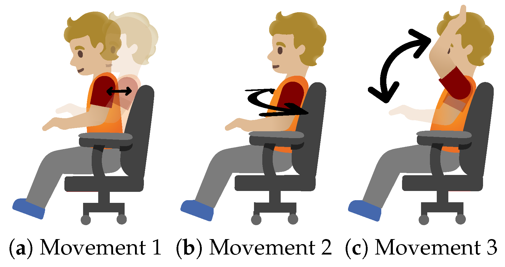
Figure 1. Illustration of the movements included in the protocol.
Information 15 00584 g001
Figure 2. System setup and experiment environment.
Information 15 00584 g002
Figure 3. Raw signal acquired by Bio-Radar.
Information 15 00584 g003
Figure 4. Optimization parameter methods.
Information 15 00584 g004
Figure 5. Results of K-mean implementation.
Information 15 00584 g005
Figure 6. Elbow method results.
Information 15 00584 g006
Figure 7. Results of DBSCAN implementation.
Information 15 00584 g007
Figure 8. Illustration of the radar signal in the complex domain with and without random motion.
Information 15 00584 g008
Figure 9. Block diagram of the algorithm.
Information 15 00584 g009
Figure 10. DBScan example for MinPts = 3.
Information 15 00584 g010
Figure 11. Optimal ε for Subject 7 with MinPts 13.
Information 15 00584 g011
Figure 12. DBScan results in the time domain.
Information 15 00584 g012
Figure 13. Polar plot DBScan results.
Information 15 00584 g013
Figure 14. Variation of the average F1 Score with MinOnesPercentage.
Information 15 00584 g014
Figure 15. Polar plot results after noise segmentation.
Information 15 00584 g015
Figure 16. Time results after noise segmentation.
Information 15 00584 g016
Table 1. Subject description.
Dataset NumberSubjectGenderBMI (kg/m2)
11F21.6
2F19.4
21M23.6
2F18.7
3M30
4M24.4
5F21.6
6M20.4
7M22.26
8F20.82
M—Male, F—Female, BMI—Body Mass Index.
Table 2. Optimal values for the k parameter.
Subject 1Subject 2Subject 3Subject 4
 k2532
Best Silhouette Score0.4880.4420.4080.587
Table 3. Optimal parameters for ϵ and minimum sample parameters.
Subject 1Subject 2Subject 3Subject 4
  ϵ 0.110.140.140.14
 Minimum Samples80787680
Best Silhouette Score0.3590.2970.5230.061
Table 4. Optimized parameters for specific movement sequences of each subject.
MinPts ε F1 ScorePrec.RecallMovement
Subject 1710.00150.770.820.691
Subject 2900.00090.770.690.863
Subject 3390.00120.680.530.711
Subject 4220.00630.850.770.943
Subject 530.00130.630.540.582
Subject 6590.00460.700.760.631
Subject 7130.00080.600.560.592
Subject 870.00050.780.930.632
Table 5. Results after noise segmentation.
F1 ScorePrecisionRecall
Subject 10.870.880.86
Subject 20.840.760.94
Subject 30.810.830.79
Subject 40.960.921
Subject 50.800.900.72
Subject 60.900.980.82
Subject 70.800.700.93
Subject 80.9310.87
Table 6. Average results for MinPts = 4 of all subjects for each movement type.
MovementAverage Values
ε F1 ScorePrecisionRecall
10.000480.830.810.87
20.000350.730.700.79
30.000290.80.730.9
Disclaimer/Publisher’s Note: The statements, opinions and data contained in all publications are solely those of the individual author(s) and contributor(s) and not of MDPI and/or the editor(s). MDPI and/or the editor(s) disclaim responsibility for any injury to people or property resulting from any ideas, methods, instructions or products referred to in the content.