KEGGSum: Summarizing Genomic Pathways

Abstract

Over time, the renowned Kyoto Encyclopedia of Genes and Genomes (KEGG) has grown to become one of the most comprehensive online databases for biological procedures. The majority of the data are stored in the form of pathways, which are graphs that depict the relationships between the diverse items participating in biological procedures, such as genes and chemical compounds. However, the size, complexity, and diversity of these graphs make them difficult to explore and understand, as well as making it difficult to extract a clear conclusion regarding their most important components. In this regard, we present KEGGSum, a system enabling the efficient and effective summarization of KEGG pathways. KEGGSum receives a KEGG identifier (Kid) as an input, connects to the KEGG database, downloads a specialized form of the pathway, and determines the most important nodes in the graph. To identify the most important nodes in the KEGG graphs, we explore multiple centrality measures that have been proposed for generic graphs, showing their applicability to KEGG graphs as well. Then, we link the selected nodes in order to produce a summary graph out of the initial KEGG graph. Finally, our system visualizes the generated summary, enabling an understanding of the most important parts of the initial graph. We experimentally evaluate our system, and we show its advantages and benefits.

1. Introduction

Molecular interactions are a large scientific chapter that includes multiple complex procedures involving a large number of sequences of actions. Glycolysis, the biosynthesis of amino acids, and caffeine metabolism are just a few examples. However, these are complex processes with numerous components that are difficult to follow or describe. The information that they carry is more easily transmitted through visual or computerized means that condense it into forms that are easier to perceive and analyze.

KEGG pathways are mostly manually drawn pathway maps representing our knowledge of the molecular interaction, reaction, and relation networks for metabolism, genetic, and environment information processing, cellular processes, organismal systems, human diseases, and drug development. KEGG pathways offer a valuable means to analyze genomes [1], to analyze and predict protein stability [2], and to identify deregulated pathways [3] and key molecular players in cancer [4] and, as such, their effective processing and understanding are of key importance. In many cases, however, those diagrams are huge, spanning over 1000 nodes, limiting the visual comprehensibility for humans. As such, the development of tools for enabling their exploration is of high importance to the field.

The information included in these pathway maps is exposed using the KEGG Markup Language (KGML), an exchange format for KEGG graph objects. Only specialized computational tools capable of taking these types of data as input and producing an output can extract conclusions from them. Pathway analysis algorithms are implemented on a daily basis so that the scientific community can deal with the massive number of data produced every second around the world. The new algorithms must be robust, employ novel computational ideas, and be capable of analyzing large numbers of data in a short period of time.

In this paper, we present KEGGSum a system that automatically downloads and analyzes KGML files directly from the KEGG database using the corresponding REST-style API. KEGGSum is able to analyze the entire graph, rapidly identifying the most important parts of these huge diagrams, allowing the researchers to better focus on the important parts of the diagrams, and facilitating their exploration. More specifically, our contributions in this paper are the following:

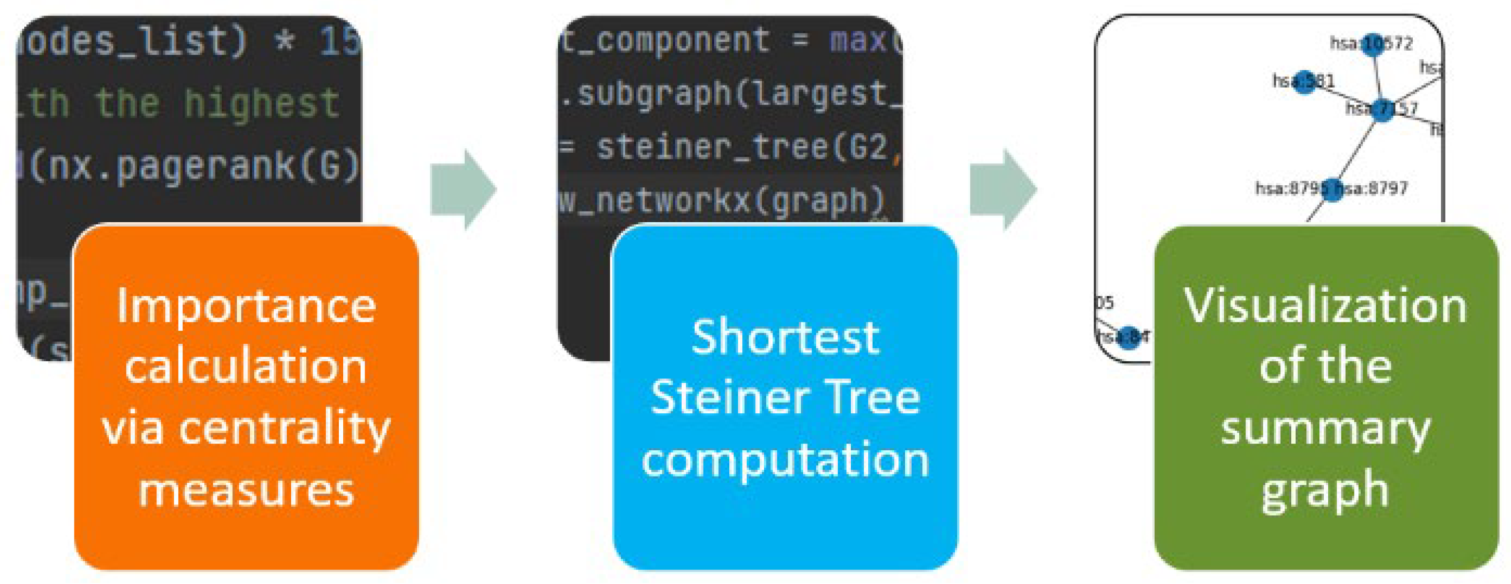
• We explore seven centrality measures (betweenness centrality, degree centrality, closeness centrality, PageRank centrality, Katz centrality, eigenvector centrality, and harmonic centrality) proposed in graph theory for capturing the importance of the graph nodes, examining their applicability to KEGG graphs as well.
• Besides identifying the most important nodes of the KEGG graphs, we link those nodes in order to present to the users a summary, i.e., a subgraph out of the original graph. In order to do so, we model the problem of summary generation as a Steiner tree problem, an approach commonly adopted for semantic summaries but not yet explored for KEGG graphs.
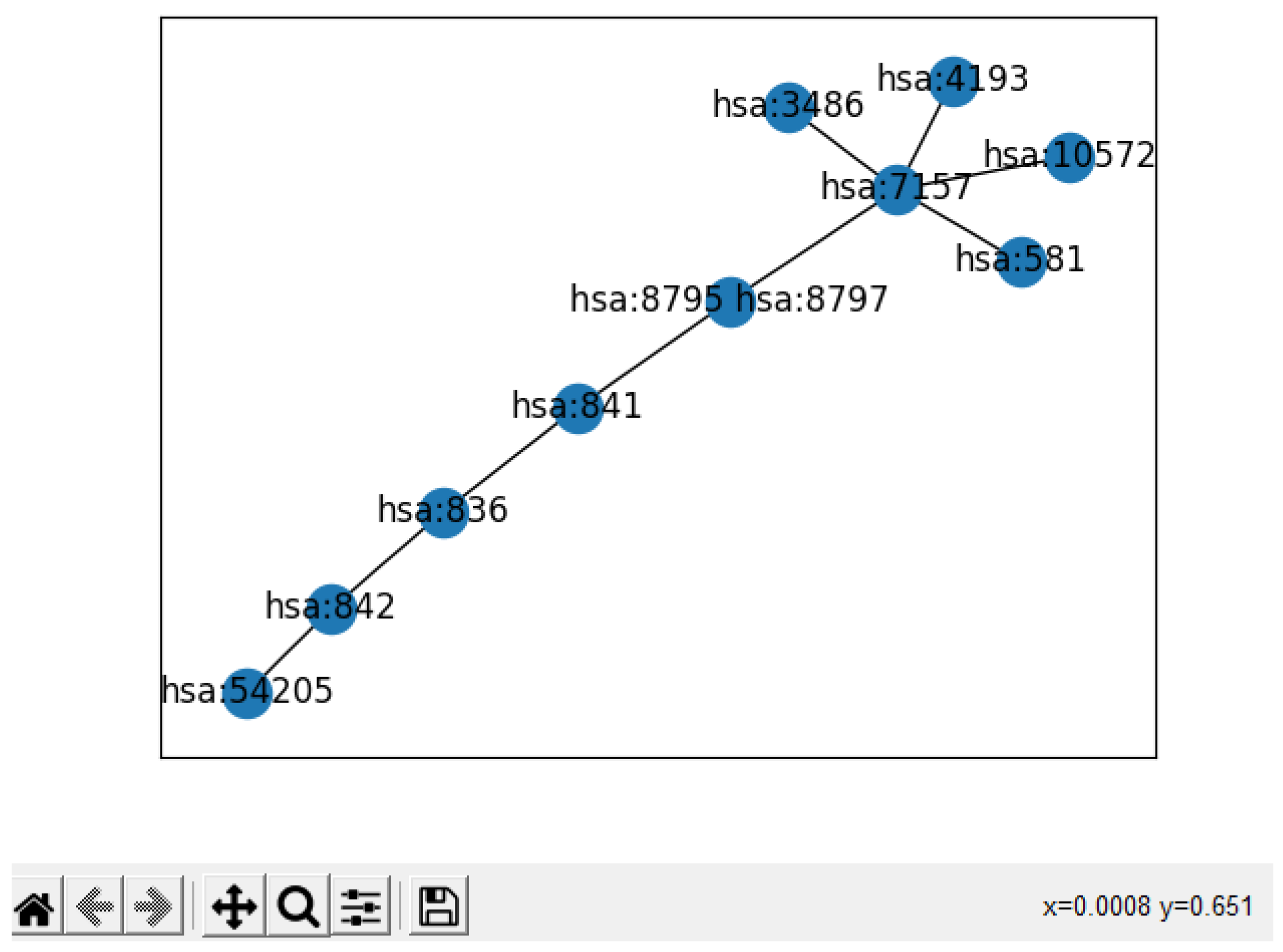
• We present a proof-of-concept visualization of the result summary, showing the researchers the most important subgraph from the original KEGG graph.
• Finally, we conduct an experimental investigation into the quality of the generated summary using three experts, identifying the usefulness of our approach. Our approach is able to select construct summaries with higher quality than using a competitive centrality measure proposed for biological networks, whereas it runs one order of magnitude faster.

To the best of our knowledge, this is the first work that proposes structural summaries for KEGG graphs. The remainder of this thesis is structured as follows: Section 2 builds the theoretical background of our research and presents related work, Section 3 describes the process of KEGG graph summarization, Section 4 contains the evaluation procedures that we followed in order to validate our results and, finally, Section 5 concludes the thesis and presents directions for future work.

2. Background

2.1. KEGG

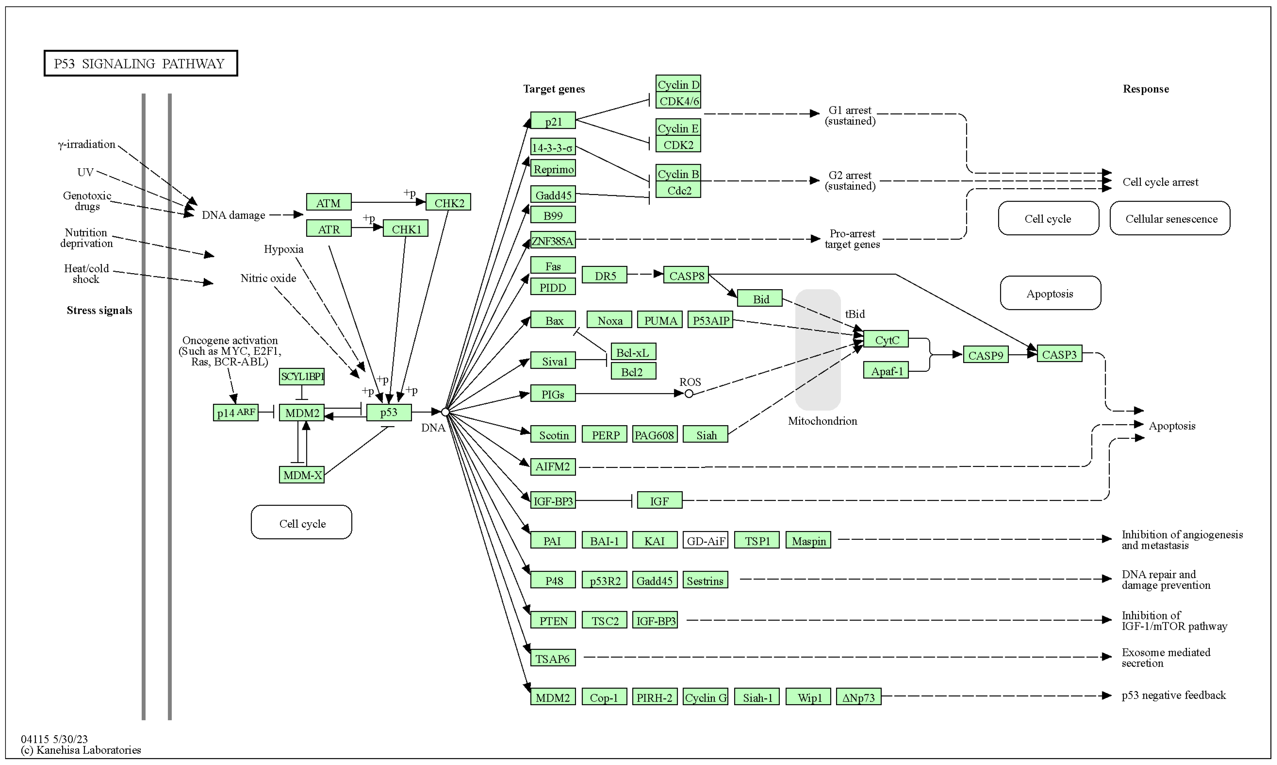
2.1.1. Pathway Maps

From genomic and molecular-level information, KEGG is a database resource for understanding the high-level functions and utilities of biological systems, such as the cell, the organism, and the environment. It is a computer representation of a biological system made up of molecular building components such as genes and proteins (genomic information) and chemical substances (chemical information) that are combined with knowledge about molecular wiring diagrams of interaction, reaction, and relation networks (system information). It also includes disease and drug information (health information), as well as biological system perturbations.

The KEGG pathway maps are graphical image maps representing the networks of interacting molecules responsible for specific cellular functions. There are two types of KEGG pathways:

• Reference pathways, which are manually drawn;
• Organism-specific pathways, which are computationally generated based on reference pathways (https://www.genome.jp/, accessed on 12 December 2023).

An example KEGG graph depicting the p53 signaling pathway for humans is shown in Figure 1.

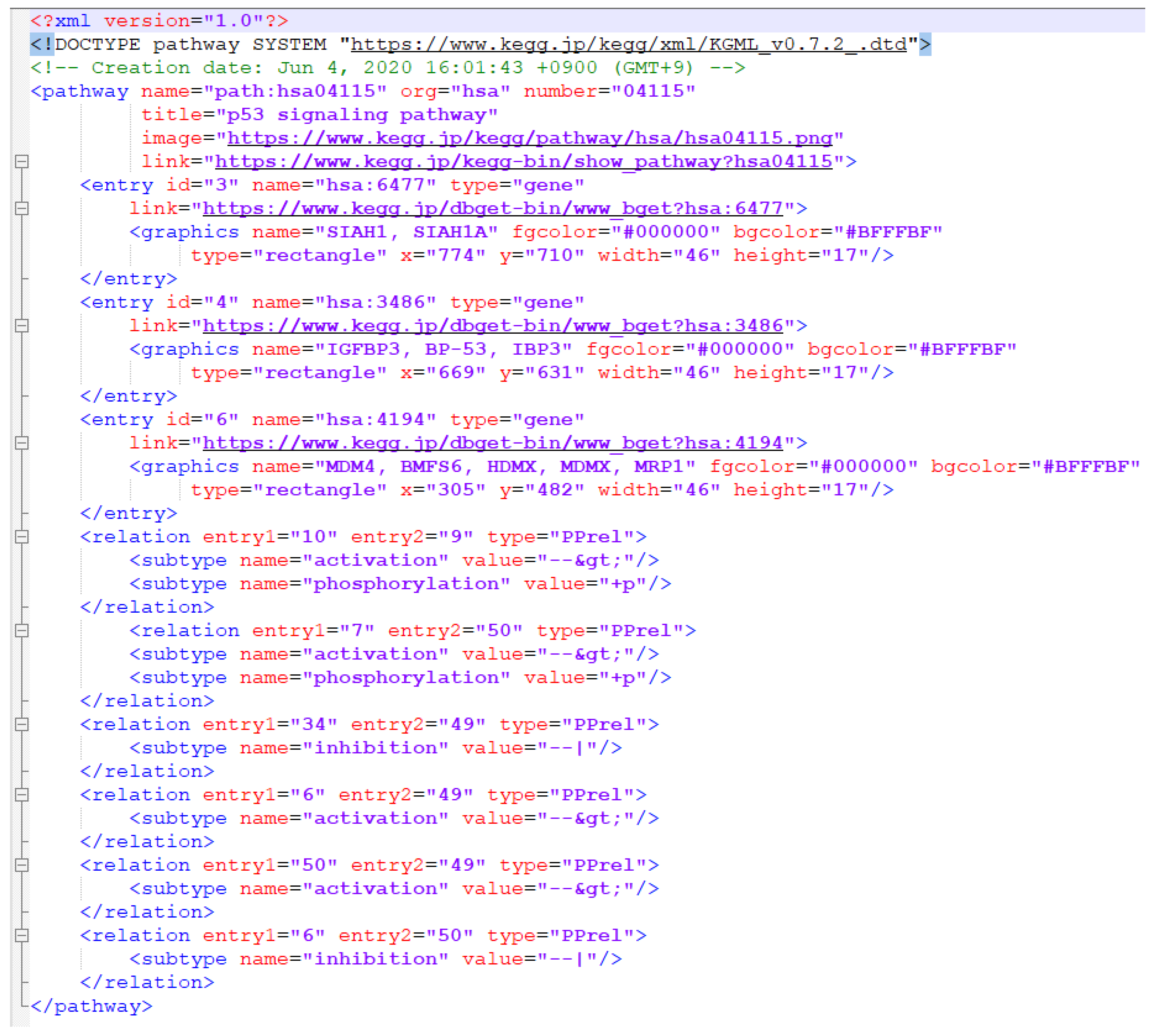
2.1.2. XML Representation of KEGG Pathway Maps

The KEGG Markup Language (KGML) is a KEGG pathway map exchange format that is converted from the internally used KGML+ (KGML+SVG) format. KGML allows for the automatic creation of KEGG pathways, as well as the computational analysis and modeling of gene/protein and chemical networks. The following are the prefixes for the pathway map identifiers:

• ko—reference pathway map linked to KO entries (K numbers);
• rn—reference pathway map linked to REACTION entries (R numbers);
• ec—reference pathway map linked to ENZYME entries (EC numbers);
• org (three- or four-letter organism code)—organism-specific pathway map linked to GENES entries (gene IDs).

The KEGG pathway maps are exchanged in KGML format. They are intended for external users and are not used by KEGG in any service or database update mechanism. KGML files are computationally created from the manually defined KGML+ file and provide information about entries (KEGG objects) and two types of relationships:

• Relations—relationships between boxes;
• Reactions—relationships between circles.

The KGML files contain computerized information about graphical objects and their relations in the KEGG pathways, as well as information about orthologous gene assignments in the KEGG GENES database.

The pathway element in KGML describes a single graph object with entry elements as nodes and relation and reaction elements as edges. In the KEGG pathways, the relation and reaction elements represent the connecting patterns of rectangles (gene products) and circles (chemical compounds), respectively. The protein network and the chemical network are two types of graph objects: those with entry and relation elements and those with entry and reaction elements, respectively. Another KEGG pathway distinction is that the metabolic pathway can be considered as both a network of proteins (enzymes) and a network of chemical substances. A snippet of a KGML file is shown in Figure 2.

2.2. Graph Theory

In the science of mathematics, graph theory is the study of graphs. A graph G = (V, E) is a discrete structure consisting of a vertex set V and an edge set E. A graph consists of a set of points and a set of lines joining some of these points. The points are the vertices, or nodes as they are commonly called, of the graph, and the lines are the edges between the vertices. The vertex set of a graph G is denoted by V(G), and its edge is set by E(G). When the graph under consideration is clear, we omit G and use V and E for the vertex and edge sets of graph G. The order of a graph G is the number of its vertices, and its size is the number of its edges [5].

In our approach, we consider a KEGG graph as a generic graph, where all KEGG objects are considered as nodes, and relationships (relations and reactions) are considered as edges. This naïve approach has already been adopted by other works in the past (e.g., [6]) and, as shown in this paper, works well in practice.

2.3. Graph Summarization and Semantic Graph Summarization

Graph summarizing has five major obstacles, according to a survey conducted by [6]: (a) a reduction in data volume to allow for more efficient analysis and the manipulation of data complexity due to the number of details and levels that entities (nodes) in a network may contain; (b) a subjective definition of interestingness that varies by case and requires both domain knowledge and user preferences to determine; (c) an evaluation of the summarization output that, in order to be good, must support both global and local queries with high accuracy; and (d) evolution—change over time necessitates that graph summaries evolve over time, as real data are frequently dynamic.

Besides summarizing generic graphs, where no special relationships are permitted between the nodes, another active field of research is summarizing graphs with richer relationships, such as semantic graphs [7]. In this domain, the existing summarization proposals are most effectively categorized from a scientific standpoint according to the main algorithmic notion underpinning the summation method:

• Structural methods take into account the graph structure first and foremost, i.e., the pathways and subgraphs encountered in the RDF graph. Because structural conditions are so important in applications and graph uses, graph structure is heavily used in summarization techniques.
  • Quotient: quotient summaries use equivalence relations between the nodes and then assign a representative to each class of equivalence in the original graph. Because each graph node can only belong to one equivalence class, structural quotient methods ensure that each graph node is represented by only one summary node.
  • Non-quotient: additional approaches to structurally summarizing semantic graphs rely on other metrics, such as centrality, to select and connect the most essential nodes in the summary.
• Pattern-mining methods: these methods make use of data-mining techniques to find patterns in the data, which are then used to construct the summary.
• Statistical methods: these methods quantitatively summarize the contents of a graph. The emphasis is on counting occurrences, such as counting class instances or creating value histograms by class, property, and value type; other quantitative measurements include the frequency of use of specific attributes, vocabularies, average string literal length, and so on. Statistical methods can also be used to investigate (usually minor) graph patterns, but only from a quantitative, frequency-based perspective.
• Hybrid methods: hybrid approaches integrate structural, statistical, and pattern-mining techniques fall into this category.

As KEGG pathways involve special relationships between the nodes, and we would like to extract a subgraph out of the original graph, our KEGGSum can be classified as a structural, non-quotient approach.

2.4. Centralities for KEGG Graphs

Although, currently, there is no other work available focusing on summarizing KEGG pathways, there is a related work revisiting graph centrality models for biological pathway analysis. The work [8] argues that typical conventional network centrality measures do not adequately capture the informative topological arrangements of pathways, limiting biological inference. They introduce source/sink centrality (SSC), a directed graph paradigm that addresses the shortcomings of traditional models. SSC measures a node’s importance as a sender and receiver of biological signals separately in the upstream and downstream of a pathway and then combines the two terms to determine its centrality.

In our experiment section, we contrast our approach with the aforementioned work only in the node-selection part, showing that, indeed KEGGSum, is able to better select the most important nodes and is more efficient. Nevertheless, KEGGSum proceeds to formulate complete summaries and goes beyond simple node selection.

3. The KEGGSum Algorithm

The KEGGSum system requires a KEGG identifier (Kid). Then, it uses KEGG’S REST API in order to download the corresponding KGML file. Then, after a preprocessing step, it calculates each node’s importance through the PageRank centrality measure, by default, or any of the seven selected centrality measures, if selected by the user. Subsequently, it isolates a percentage (15% by default) of the most important nodes out of the total node population and links them in a whole subgraph extracted out of the initial KEGG graph Finally, it visualizes the new graph as the original pathway’s summary graph. An overview of the whole process is shown in Figure 3.

3.1. Pre-Processing

The algorithm has been configured in such a way that it may be used as a function. After the “kid” is provided by the user during the function call, KGML files are retrieved automatically from the algorithm. The pathways, most of the time, include nodes non-significant to the insight extraction process. These nodes need to be removed from the data in order to cleanse the data and proceed with the pre-processing. The pre-processing steps that are executed on the retrieved data by the algorithm are the following:

• Filtering of chemical substrates and reactions. In our effort to create a more dense but rapidly comprehensible graph, we need to deal with the most significant and relevant, down to the final result, data. The main idea of the summarization process concerns the visualization of a number of significant genes. For this reason, nodes that represent chemical substrates and edges that represent reactions need to be filtered out.
• Filtering of orthologs. The KEGG pathway files sometimes include genes orthologous to the significant ones. These nodes signify genes that have similar functions in other organisms. But, for the cause of pathway summarization, they consist of data noise, which cannot be computationally processed, so they are filtered out, too, at the pre-processing stage.
• Filtering of nodes characterized as “undefined”. Sometimes, KEGG pathways have an undefined sequence as a node. These sequences’ accession numbers are, consequently, characterized as “undefined” and are of no value to the summarization process of the pathway. Thus, they are removed.

3.2. Centrality Measures Explored

The node-evaluation phase of the KEGGSum algorithm uses several centrality metrics. Despite the fact that KEGGSum, by default, uses PageRank, seven centrality measures were investigated in order to identify the one with the best performance. A centrality measure is a function c: G(n)→Rⁿ, where c_i(v) is the centrality i of the node v in the network G. The centrality measures we explored are:

Betweenness centrality: Freeman’s betweenness centrality measures the importance of a node in connecting other nodes in the network. It considers all geodesics between two nodes j and k, different from v, that pass through v. The betweenness centrality thus captures the role of an agent as an intermediary in the transmission of information or resources between other agents in the network. As there may be multiple geodesics connecting j and k, we need to keep track of the fraction of geodesic paths passing through v. The betweenness centrality measure proposed by [9] is:

$$C_{\mathrm{Betweenness} }(v)=\sum _{v\ne t}\frac{{\sigma }_{\mathit{st}}(v)}{{\sigma }_{\mathit{st}}}$$

where σ_st is the total number of shortest paths (of the same minimal length) from node s to node t, and σ_st(v) is the number of those paths that pass through v.

Degree centrality measures the number of edges of node v, d(v). We can also normalize by the maximal possible degree, n − 1, to obtain a number between 0 and 1:

$$C_{\mathrm{Degree}}(v)=\frac{d(v)}{n-1}$$

Degree centrality is an obvious centrality measure and gives some insight into the connectivity or “popularity” of node i, but misses potentially important aspects of the architecture of the network and a node’s position in it [10].

Closeness centrality is based on the network distance between a node and each other node. It extends degree centrality by looking at the neighborhoods of all radii. The input into measures of closeness centrality is the list of distances between node v and other nodes j in the network, d(j,v). There are different variations in the closeness centrality based on different functional forms. The measure proposed by [11,12] is based on the distances between node v and all other nodes. In this measure, a higher score indicates a lower centrality. To deal with this inversion, and also to deal with the fact that this distance becomes infinite if nodes belong to two different components, the study [12] proposed a centrality measure of $\frac{1}{{\displaystyle {\sum }_j}d(j,v)}$. One can also normalize that measure so that the highest possible centrality measure is equal to 1 to obtain the closeness centrality measure, assuming n to be the number of nodes in the graph.

$$C_{\mathrm{Closeness} }(v)=\frac{n-1}{{\displaystyle {\sum }_{v\ne j}}d(j,v)}$$

An alternative measure of closeness centrality (e.g., see [13,14]) aggregates distances differently. It aggregates the sum of all inverses of distances. This avoids having a few nodes for which there is a large or infinite distance to drive the measurement.

PageRank centrality was introduced originally by Google to rank web pages. It simulated the behavior of users when browsing the Web to rank pages, where pages are graph nodes, and hyperlinks are edges. PageRank denotes the ‘importance’ of nodes under the assumption that the importance of a node is the expected sum of the importance of all connected nodes and the direction of edges. Its value corresponds to the probability distribution of nodes being accessed at random. In graph theory, PageRank computes, recursively, a normalized and propagated value for each node in a graph.

Let x and p be two nodes in a graph G; the PageRank of x is given as follows:

$$C_{\mathrm{PageRank}}(v)=(1-c)+c.\sum _{p\in P_{\mathrm{in} }(v)}\frac{\mathit{PR}(p)}{\left|P_{\mathrm{out} }(p)\right|}$$

where c is a damping factor that takes its value in [0,1] (typically 0.85), P_in(x) is the set of nodes pointing to x, and P_out(p) is the set of nodes pointed by p and |P_out(p)| is its cardinality [15].

Katz centrality measures the relative influence of each node in a given network by taking into account its immediate neighboring nodes, as well as non-immediate neighboring nodes that are connected through immediate neighboring nodes. The Katz centrality of a node v_i is computed as:

$$C_{\mathrm{Katz} }\left(v\right)=\alpha {\displaystyle \sum _{j=1}^n}{A}_{j,i}{C}_{\mathrm{Katz} }\left(v_j\right)+\beta$$

where α is a constant called the damping factor, usually considered to be less than the largest eigenvalue, λ, i.e., α < 1/λ, and β is a bias constant, also called the exogenous vector, used to avoid the zero centrality values. With α ≥ λ, the centrality tends to diverge [16]. In our implementation, we used the default values for the constants, as proposed in the NetworkX library, i.e., α = 0.1, β = 1.0.

Eigenvector centrality is a related measure of prestige [17]. It relies on the idea that the prestige of node v is related to the prestige of its neighbors. The eigenvector centrality is computed by assuming that the centrality of node v is proportional to the sum of the centrality of the nodes’ neighbors:

$$C_{\mathrm{Eigenvector}}\left(v\right)=\frac{1}{\lambda }{\displaystyle \sum _{t \in {\rm M}(v)}}{x}_t=\frac{1}{\lambda }\sum _{t\in V}{a}_{v,t}{x}_t$$

where a_v,t is the adjacency matrix, i.e., a_v,t = 1 if vertex v is linked to vertex t, and 0 otherwise; M(v) is the set of neighbors of v; and λ is a constant. The eigenvector centrality of a node is, thus, self-referential but has a well-defined fixed point. This notion of centrality is closely related to ways in which scientific journals are ranked based on citations and also relates to influence on social learning [10].

Harmonic centrality: for each graph-theoretical notion based on arithmetic averaging or maximization, there is an equivalent notion based on the harmonic mean. If we consider closeness the reciprocal of a denormalized average of distances, then it is natural to also consider the reciprocal of a denormalized harmonic mean of distances. We thus define the harmonic centrality of v as

$$C_{\mathrm{Harmonic}}\left(v\right)={\displaystyle \sum _{y\ne v}}\frac{1}{d(y,v)}=\sum _{d(y,v)<\mathrm{\infty },y\ne v}\frac{1}{d(y,v)}$$

Harmonic centrality is strongly correlated to closeness centrality in simple networks, but naturally also accounts for nodes y that cannot reach v. Thus, it can be fruitfully applied to graphs that are not strongly connected [18].

The time complexity of those algorithms is depicted in

Table 1. Time complexities of the explored centrality measures.

Measure	Complexity
Betweenness	O (V × (V × E))
Degree	O (V+E)
Closeness	O (V × E)
PageRank	O (k × E)
Katz	O (V3)
Eigenvector	O (V × logV
Harmonic	O (N × (N+E))

, where V denotes nodes (vertices), E denotes edges, and k denotes the number of iterations. The selection of these specific centralities was based on similar works from the semantic summarization field [19], where these specific centralities showed a good performance on summarizing semantic graphs, and also in the relevant literature focusing on centralities for biological pathway analysis [8]. Based on their centralities, centralities with a small complexity, like the degree centrality, would allow their efficient computation, whereas centralities with high complexity, such as the betweenness centrality, might eventually become infeasible in big graphs due to the large time required for their computation.

3.3. Linking the Most Important KEGG Nodes

As soon as the most important nodes are identified, they are passed to the next module of the system in order to be linked. To link these nodes, as commonly performed in semantic summaries [19], we view the problem as a Steiner tree problem that tries to link the aforementioned nodes with as few as possible additional nodes.

The graph Steiner tree problem (GSTP): given an undirected graph G = (V, E), with edge weights w: E → ℝ + and a node set of terminals S ⊆ V, find a minimum-weight tree T ∈ G such that S ⊆ Vt and Et ⊆ E.

In our case, all nodes and edges have an equal weight, so the objective is to introduce the smallest number of additional nodes in the result graph. The problem is known to be NP-complete and, as such, an approximation algorithm is used (CHINS) [20] with a complexity of O(Q · (V + E)), where Q is the number of nodes to be linked.

3.4. The KEGGSum Algorithm

Briefly, the KEGGSum algorithm downloads and parses a KGML file from the KEGG database, identifies its most important nodes, connects them into a summary graph, and visualizes the graph summary, as described in Algorithm 1.

Algorithm 1. KEGGSum. Creates graph summaries of KEGG graphs

Input: kid—a KEGG Identifier, perc—percentage of important nodes to isolate, cent—centrality measure with which to determine the importance of the nodes.

Output: A summary graph.

1. File: = download(kid) //Download and parse the KGML file based on kid

2. Nodes: =Identify_most_important_nodes(perc, cent) //identify the perc most important nodes based on the cent centrality measure

3. Graph: = Steiner_Tree(File, Nodes) //connects the most important nodes using he Steiner Tree algorithm

4. Visualize(Graph) //visualizes the graph summary

The time complexity of KEGGSum depends on the complexities of the algorithms of the various components used, i.e., for calculating the nodes’ centrality and the Steiner tree algorithm.

Since the centrality that appeared to perform best in the experimentation stage was PageRank centrality, its time complexity is used to calculate KEGGSum’s time complexity:

$$O\left(\mathrm{Q}·(\mathrm{V}+\mathrm{E})+k·E\right)$$

In KEGGSum’s function call, the user provides the pathway KEGG identifier for which they want to produce the graph summary. The important node percentage can be customized through the argument “perc”, which denotes percentage, and the centrality method is to be used by the argument “cent”, which denotes centrality. The available options for the “cent” argument are: “Betweenness”, “Degree”, “Closeness”, “PageRank”, “Katz”, “Eigenvector”, and “Harmonic”.

4. Evaluation

The Integrated Development Environment (IDE) PyCharm was used to develop KEGGSum on a system running Python 3.9.10. In terms of the visualization of the summary graph, the “Bio” and “networkx” libraries were imported and utilized, as well, for the analysis of the KGML files and the centrality measure calculations. All the aforementioned centrality measures are available through KEGGSum, where, by default, the PageRank is used. The source code of our system is available online on GitHub (https://github.com/chaimdavid/keggsum, accessed on 15 January 2024).

Next, we present the methodology followed for evaluating KEGGsum using three domain experts.

4.1. Datasets

In order to evaluate our approach, we reused the dataset available in [8]. More specifically, out of the entire dataset, we carefully selected ten pathways from the “human data” section in order not to congest the experts with a massive number of pathways to be examined. Further, the selected pathways had more than 50 nodes after passing the pre-processing stage.

4.2. Competitors

We compared the results on node selection with Naderi et al.’s [8] approach. In our approach, we explore seven centrality measures, contrasting the results with the centrality measure introduced by [8]. Using our approach, we are able to construct whole summary graphs; not only do we select the most important nodes as the competitor does, but we compare only the step of node selection with the competitor.

4.3. Reference Dataset Construction

We invited three pathway network experts (from now on referred to as EXP1, EXP2, and EXP3) to review our pathway dataset and carefully identify 15% of critical nodes for each pathway so that we could evaluate the outcomes that our algorithm produces. The pathway network experts were given the pathways, along with the number of most important nodes that they should identify corresponding to this 15% of the overall nodes.

We analyzed the inter-rater reliability [21] of the pathway network experts (raters) using Cohen’s kappa [22,23], in order to calculate the degree of agreement between them and validate the reference dataset’s credibility. The average inter-rater reliability is 0.47 and is moderate (0.41–0.60), going beyond fair (0.21–0.40), but lower than substantial (0.61–0.80).

4.4. Metrics

We evaluated our algorithm’s results on selecting the most important nodes with the conventional evaluation measures: precision, recall, and F-measure.

Precision, which quantifies the number of positive class predictions that actually belong to the positive class.

$$\mathit{Precision}=\frac{\mathit{True} \mathit{Positive}}{\mathit{True} \mathit{Positive}+\mathit{False} \mathit{Positive}}$$

Recall, which quantifies the number of positive class predictions made out of all positive examples in the dataset.

$$\mathit{Recall}=\frac{\mathit{True} \mathit{Positive}}{\mathit{True} \mathit{Positive}+\mathit{False} \mathit{Negative}}$$

F-measure, which provides a single score that balances both the concerns of precision and recall in one number.

$$F–\mathit{Measure}=2\times \frac{\left(\mathit{Precision}\times \mathit{Recall}\right)}{\mathit{Precision}+\mathit{Recall}}$$

For example, assuming that we asked one expert to identify the 10 most important nodes from a KEGG graph, and our summary returned 10 nodes, with 8 of them correctly identified, the precision would be 8/10, the recall 8/10, and the f-measure 2 × ((0.8 × 0.8)/(0.8 + 0.8)).

Further, we evaluate performance in terms of the mean execution time for each algorithm. In order to compare the execution times of the various algorithms, we calculated the average time of 50 executions up to the module of the centrality measure computation. The competitor algorithm, in one stage, connects to the database, downloads the pathway data, and saves them locally, and, in a second stage, reads the data from the local source and applies the centrality calculations. So, in order to maintain the same parameters across both algorithms and compare solely the centrality calculation module, the mean time computations were performed by parsing the datasets from a local source for them both. The experiments were performed in a Windows 10 Pro 21H2 operating system, on an Intel Core i7 4790K running at 4.00 GHz with 16.00 GB RAM running at 4.00 GHz.

4.5. Results

Figure 4, Figure 5 and Figure 6 depict the results for the three individual experts using the various centrality measures and the competitor. In each diagram, the precision, recall, and f-measure are visualized. Besides the individual experts, we also present, in Figure 7, the mean across all experts.

As shown in Figure 4, Figure 5 and Figure 6 of the individual experts, PageRank is consistently better than other centrality measures, followed by degree and betweenness. On the other hand, eigenvector and closeness seem to consistently show a bad performance. As shown, the results are similar for all experts, with small variations between EXP1 and EXP2, and slightly greater ones with EXP3. In all cases, the competing algorithm has a bad performance, with moderate recall but really bad precision, leading to a bad F-measure.

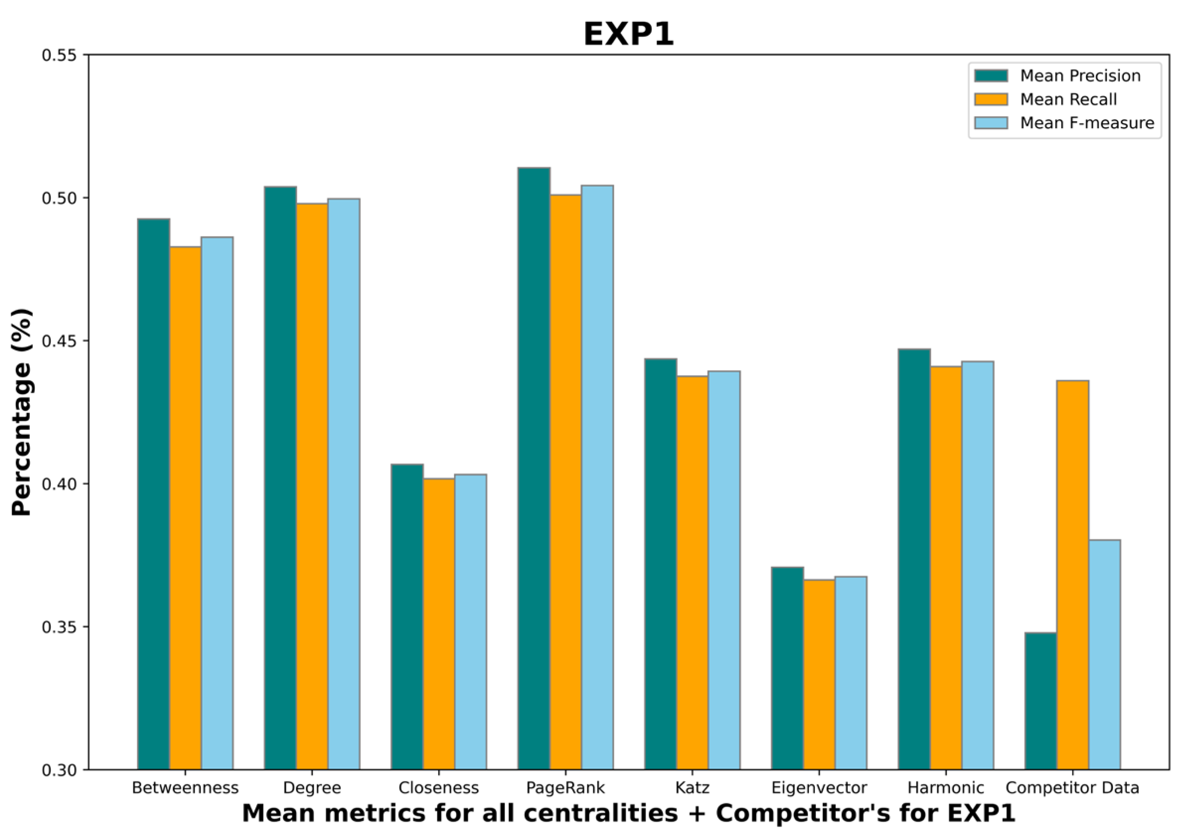
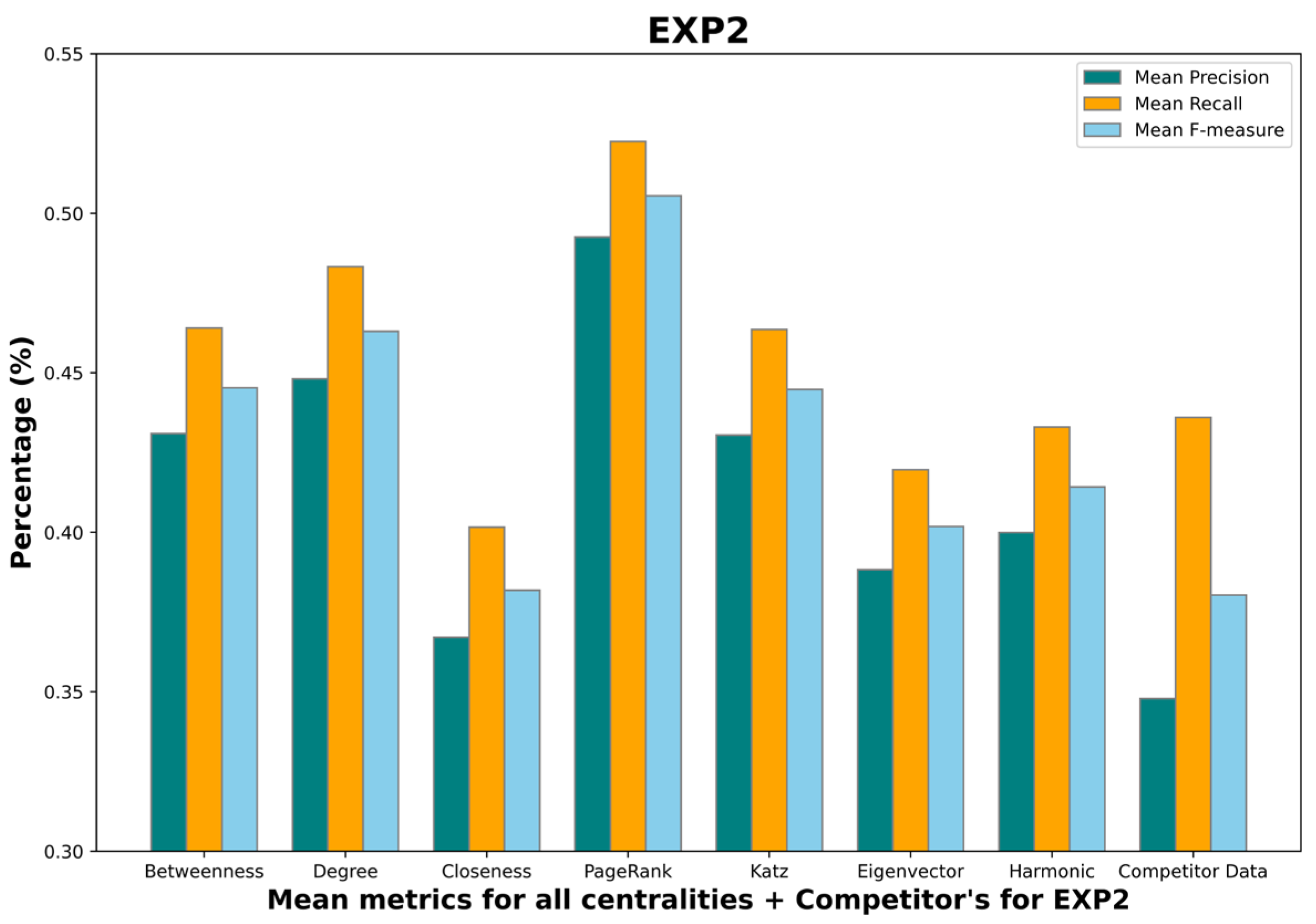
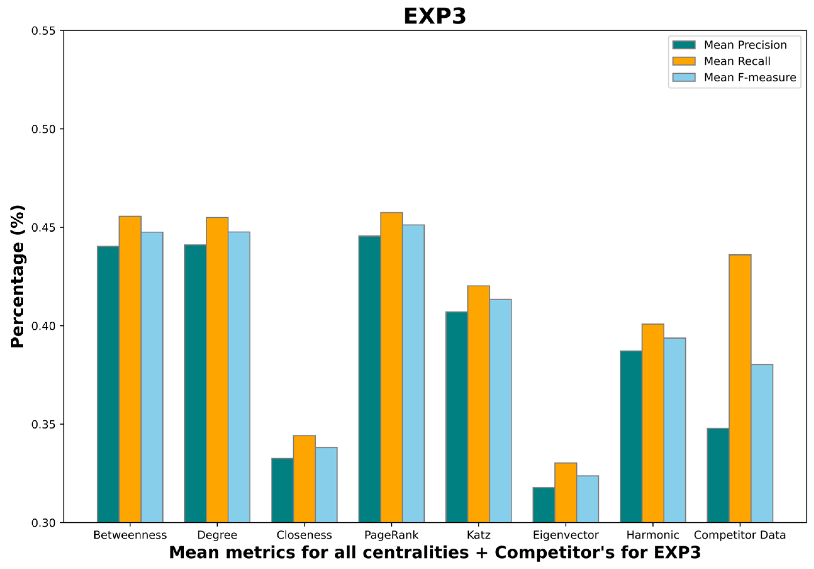
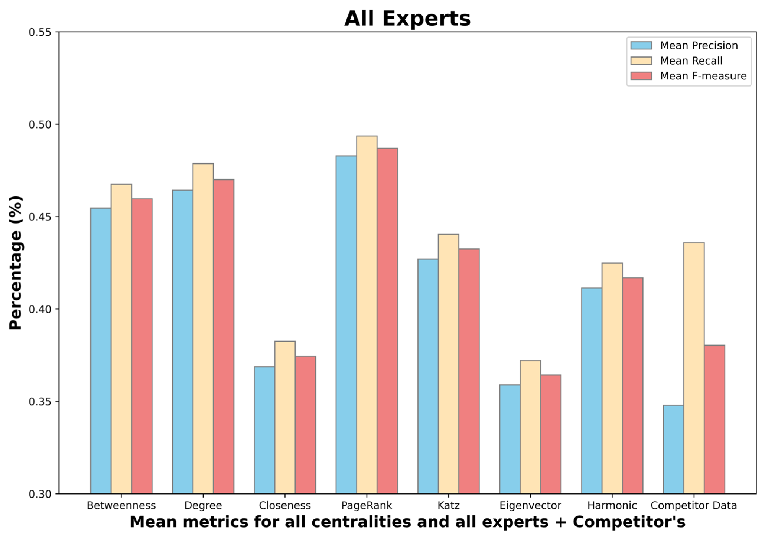
Looking at the mean results across all experts, we can see a similar tendency. While it is visually challenging to determine which performance measure is superior, due to the results of degree and PageRank centralities being so close, when we compare the mean F-measure values of all centrality measures, we see the following results:

• Mean betweenness centrality F-measure: 0.45;
• Mean degree centrality F-measure: 0.48;
• Mean closeness centrality F-measure: 0.38;
• Mean PageRank centrality F-measure: 0.48;
• Mean Katz centrality F-measure: 0.43;
• Mean eigenvector centrality F-measure: 0.36;
• Mean harmonic centrality F-measure: 0.41;
• Competitor F-measure: 0.38.

As such, according to their performance, the seven centrality measurements can be divided into three categories. The ones that performed well, like the PageRank, degree, and betweenness centralities, the ones that did moderately, like the Katz and harmonic centralities, and the ones that performed poorly, like the closeness and eigenvector centralities.

According to this categorization, the competing algorithm had a poor performance, with an F-measure metric of 0.38. The performance of the algorithm’s recall is moderate; however, the precision is rather bad, and, as such, the F-measure score is low, showing the advantages of our solution as the only approach currently trying to identify important parts over pathway graphs.

We can confidently infer that, among the seven centralities we utilized to evaluate our algorithms’ performance over the reference dataset, PageRank centrality has the best performance metrics. Further, both PageRank and degree centrality are preferable, based on their complexity. They are both feasible to compute in big graphs due to their low complexity (refer to Table 1), whereas betweenness is computationally hard to compute.

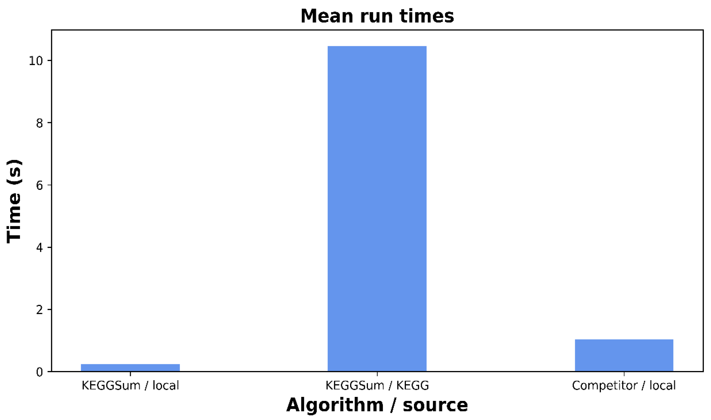
4.6. Execution Time

The mean execution time for all the 10 pathways of our dataset is shown in Figure 8. In the figure, the first column depicts the runs when the KEGG pathways are locally stored in the file system, the second column shows when the KEGG pathways are downloaded from the online KEGG database, and the third column depicts the mean execution time for the competitor that is able only able to access datasets from the local filesystem. As shown, when accessing the online database network, communication is the dominant time, leading to a total execution of 10 s, whereas the computation of the centrality using PageRank is very fast, requiring only 0.2 s when datasets are available in the local file system. On the other hand, the competitor requires ~1 s to finish calculations using the local filesystem.

Overall, KEGGsum is one order of magnitude faster than the competitor, whereas the selected most important nodes are of higher quality.

4.7. Use Case and Evaluator Comments

An example execution of the system is shown in Figure 9, demonstrating the output of system visualization. In this example, the most central node is easily identifiable (“hsa:7157”), and the other most important nodes of the graph are connected with a minimum spanning tree according to the connections they had in the original graph.

Users are able to select the centrality measure to be used, and they can pan, zoom in, or zoom out in the result graph. Further, they can click on a selected node to visit the corresponding information page provided by the KEGG library. Finally, they can save the resulting image as a file.

All experts appreciated the fact that our system is able to identify fast the most important nodes of the KEGG pathways, and this has a high utility for large networks where, in essence, it is really difficult for the experts to visually navigate them. They all appreciated the smooth user experience and the ease of use. Further, the experts expressed their wish for the visual diagrams to be closer to the original pathway diagrams in order to steepen the learning curve of KEGGSum, which we leave for future work.

5. Conclusions

In this paper, we present KEGGSum, a system that not only makes it easier to visually identify the most important elements (nodes) of a KEGG pathway, but also makes it easier to grasp the biological processes and information that it depicts. As in any project, there were difficulties to overcome, since most KEGG pathways are not exact visualizations of the KGML files that accompany them. Some of the pathway’s objects are inserted by hand, are not included in the KGML file, and cannot be computationally processed by an algorithm. But, with proper guidance, theoretical research, and perseverance, we managed to have a complete and effectual result.

To this end, we extracted a dataset of ten pathways from the KEGG database, processed it, and handed it over to a group of pathway network experts, who used their expertise and experience to help us create a reference dataset by identifying the nodes of each pathway that they deemed to be more important. In order to find the best fit for our system, we compared the performance of seven different centrality measures to the reference dataset. Also, we compared our algorithm’s performance to a competitor algorithm that was implemented under the same logic and calculated values from a plethora of centrality algorithms, too. As described in Section 4, PageRank centrality performed best against the reference dataset, and this is the centrality measure that we have set as default for KEGGSum. Naturally, any of the seven centrality metrics investigated can be selected by the user with the appropriate keywords during the function call.

Overall, KEGGSum is able to spot the most important nodes out of a big KEGG graph. In other to do this, otherwise, substantial knowledge of the domain is required, and also, a lot of time should be spent carefully examining big KEGG graphs.

Future work: although a single centrality measure has been identified as giving the best results, a combination of several of them could lead to even better results, which we intend to explore in the sequel. In this direction, machine learning methods could be explored to combine those centralities as features, or for learning to identify the most important nodes based on past selections from the experts [24]. Further, besides node selection, optimally selecting the edges in order to link the most important nodes can be further refined.

Further, we intend to make the visual diagrams produced via KEGGSum closer to the original manual-drawn diagrams of KEGG, although KEGG does not publicly offer a tool or any API for this. The user experience could also be enhanced by allowing users to select nodes from the initial diagram and then complementing user selections with nodes selected by our engine, making personalized summaries for the individual domain experts [25].

References

- Kanehisa, M.; Furumichi, M.; Sato, Y.; Kawashima, M.; Ishiguro-Watanabe, M. KEGG for taxonomy-based analysis of pathways and genomes. Nucleic Acids Res. 2023, 51, D587–D592. [Google Scholar] [CrossRef] [PubMed]
- Huang, F.; Fu, M.; Li, J.; Chen, L.; Feng, K.; Huang, T.; Cai, Y.D. Analysis and prediction of protein stability based on interaction network, gene ontology, and kegg pathway enrichment scores. Biochim. Biophys. Acta (BBA)-Proteins Proteom. 2023, 1871, 140889. [Google Scholar] [CrossRef] [PubMed]
- Yousef, M.; Ozdemir, F.; Jaber, A.; Allmer, J.; Bakir-Gungor, B. PriPath: Identifying dysregulated pathways from differential gene expression via grouping, scoring, and modeling with an embedded feature selection approach. BMC Bioinform. 2023, 24, 60. [Google Scholar] [CrossRef] [PubMed]
- Thippana, M.; Dwivedi, A.; Das, A.; Palanisamy, M.; Vindal, V. Identification of key molecular players and associated pathways in cervical squamous cell carcinoma progression through network analysis. Proteins Struct. Funct. Bioinform. 2023, 91, 1173–1187. [Google Scholar] [CrossRef] [PubMed]
- Erciyes, K. Discrete Mathematics and Graph Theory, A Concise Study Companion and Guide; Springer Nature Switzerland: Cham, Switzerland, 2021. [Google Scholar] [CrossRef]
- Liu, Y.; Safavi, T.; Dighe, A.; Koutra, D. Graph summarization methods and applications: A survey. ACM Comput. Surv. 2018, 51, 1–34. [Google Scholar] [CrossRef]
- Cebiric, Š.; Goasdoué, F.; Kondylakis, H.; Kotzinos, D.; Manolescu, I.; Troullinou, G.; Zneika, M. Summarizing semantic graphs: A survey. VLDB J. 2018, 28, 295–327. [Google Scholar] [CrossRef]
- Naderi Yeganeh, P.; Mostafavi, M.T.; Richardson, C.; Saule, E.; Loraine, A. Revisiting the use of graph centrality models in biological pathway analysis. BioData Mining 2020, 13, 5. [Google Scholar] [CrossRef] [PubMed]
- Freeman, L.C. A Set of Measures of Centrality Based on Betweenness. Sociometry 1977, 40, 35–41. [Google Scholar] [CrossRef]
- Bloch, F.; Jackson, M. Centrality Measures in Networks. SSRN Electron. J. 2016. [Google Scholar] [CrossRef]
- Bavelas, A. Communication patterns in task-oriented groups. J. Acoust. Soc. Am. 1950, 22, 725–730. [Google Scholar] [CrossRef]
- Sabidussi, G. The centrality index of a graph. Psychometrika 1966, 31, 581–603. [Google Scholar] [CrossRef]
- Garg, M. Axiomatic Foundations of Centrality in Networks. SSRN Electron. J. 2009. [Google Scholar] [CrossRef]
- Rochat, Y. Closeness Centrality Extended to Unconnected Graphs: The Harmonic Centrality Index; ASNA: Zurich, Switzerland, 2009. [Google Scholar]
- Henni, K.; Mesghani, N.; Gouin-Vallerand, C. Unsupervised graph-based feature selection via subspace and pagerank centrality. Expert Syst. Appl. 2018, 114, 46–53. [Google Scholar] [CrossRef]
- Zhan, J.; Gurung, S.; Parsa, S. Identification of top-K nodes in large networks using Katz centrality. Big Data 2017, 4, 16. [Google Scholar] [CrossRef]
- Zaki, M.J.; Meira, W. Data Mining and Analysis: Fundamental Concepts and Algorithms; Cambridge University Press: New York, NY, USA, 2014. [Google Scholar]
- Bolid, P.; Vigna, S. Axioms for Centrality. Internet Math. 2014, 10, 222–262. [Google Scholar] [CrossRef]
- Pappas, A.; Troullinou, G.; Roussakis, G.; Kondylakis, H.; Plexousakis, D. Exploring Importance Measures for Summarizing RDF/S KBs. In Proceedings of the European Semantic Web Conference, Portorož, Slovenia, 28 May–1 June 2017; pp. 387–403. [Google Scholar] [CrossRef]
- Dreyfus, S.E.; Wagner, R.A. The steiner problem in graphs. Networks 1971, 1, 195–207. [Google Scholar] [CrossRef]
- Gwet, K. Handbook of Inter-Rater Reliability: The Definitive Guide to Measuring the Extent of Agreement among Raters; Advanced Analytics, LLC: Gaithersburg, MD, USA, 2014. [Google Scholar]
- Landis, R.J.; Koch, G.G. The Measurement of Observer Agreement for Categorical Data. Biometrics 1977, 33, 159–174. [Google Scholar] [CrossRef] [PubMed]
- McHugh, M. Interrater reliability: The kappa statistic. Biochem. Medica 2012, 22, 276–282. [Google Scholar] [CrossRef]
- Trouli, G.E.; Pappas, A.; Troullinou, G.; Koumakis, L.; Papadakis, N.; Kondylakis, H. Summer: Structural summarization for RDF/S KGs. Algorithms 2022, 16, 18. [Google Scholar] [CrossRef]
- Vassiliou, G.; Alevizakis, F.; Papadakis, N.; Kondylakis, H. iSummary: Workload-Based, Personalized Summaries for Knowledge Graphs. In European Semantic Web Conference; Springer Nature Switzerland: Cham, Switzerland, 2023; pp. 192–208. [Google Scholar]