Ensemble System of Deep Neural Networks for Single-Channel Audio Separation

Abstract

Speech separation is a well-known problem, especially when there is only one sound mixture available. Estimating the Ideal Binary Mask (IBM) is one solution to this problem. Recent research has focused on the supervised classification approach. The challenge of extracting features from the sources is critical for this method. Speech separation has been accomplished by using a variety of feature extraction models. The majority of them, however, are concentrated on a single feature. The complementary nature of various features have not been thoroughly investigated. In this paper, we propose a deep neural network (DNN) ensemble architecture to completely explore the complimentary nature of the diverse features obtained from raw acoustic features. We examined the penultimate discriminative representations instead of employing the features acquired from the output layer. The learned representations were also fused to produce a new features vector, which was then classified by using the Extreme Learning Machine (ELM). In addition, a genetic algorithm (GA) was created to optimize the parameters globally. The results of the experiments showed that our proposed system completely considered various features and produced a high-quality IBM under different conditions.

1. Introduction

Both signal processing and neutral network researchers have paid a lot of attention to source separation (SS) in recent years. Source separation refers to the ability to separate a mixed signal into distinct components. Separating target speech from mixed signals is crucial for several applications, including speech communication and automatic speech recognition. From an application viewpoint, conducting speech separation by utilizing a single recorder is frequently the preferred method. To solve this difficult issue, several solutions have been proposed. The recovery (separation) of several audio sources that have been mixed into a single-channel audio signal, such as many persons talking over each other, is the challenge of single-channel audio source separation. Many methods have been suggested to solve the Single-Channel Source Separation (SCSS) issue. One of the main methods, Computational Auditory Scene Analysis (CASA), attempts to emulate the human auditory system in order to identify a variety of sound sources based on distinctive individual qualities [1,2].

A deep-neural-network-based ensemble system is suggested in this study, and ’wide’ and ’forward’ ensemble systems are used to comprehensively examine the complimentary properties of various characteristics. Additionally, the penultimate representations are looked into rather than the characteristics learnt from the output layer. The Extreme Learning Machine classification of the final embedded features produces binary masks to separate the mixed signals. The experimental findings show that the suggested ensemble system can produce a high-quality binary mask in a variety of settings.

The contributions of this paper are as follows: The Ideal Binary Mask (IBM) is estimated by using a DNN ensemble audio separation method to separate the premixed signal. Each DNN in the proposed system is trained with raw acoustic features by using a layer-wise pretraining approach. Various DNNs can extract different meaningful representations with different initializations. The multiview spectral embedding (MVSE) is used to embed the output of the penultimate layer of each individual DNN into a low-dimensional embedding [3,4,5]. The objective is to extensively investigate the aspects that complement the previously studied ones. “DNN Ensemble Embedding (DEE)” is the name of the first module. DNN Ensemble Stacking (DES) is the second module, which is a stack of DNN ensembles. The embedded features from the bottom module are concatenated with raw acoustic features to create a new feature set for each individual DNN in this module.

The DNNs in the system have the same design but different initializations for simplicity. By ensembling and stacking the input data, the proposed ensemble system is capable of completely exploring the complementary characteristics of the data and therefore generalize the learned representations with greater robustness and discriminative features than an individual DNN. As a result, even with limited training examples, the suggested system may still perform effectively. The Extreme Learning Machine (ELM) classifier is able to classify the time–frequency (TF) unit more accurately by using the learned discriminative characteristics of the ensemble system, and therefore the estimated IBM is more precise for source separation. Finally, a genetic algorithm is used to finetune the entire system settings in order to regularize any outliers learned by the DNNs and create a smooth map to increase the classification accuracy. Experiments were carried out on a limited training dataset, and the testing results showed that our proposed system could achieve a high separation performance. The proposed method has a high learning speed and high accuracy and lower computational complexity, and the separation performance is improved.

The remainder of this paper is organized as follows: The related work is presented in Section 2. The learning system is introduced in Section 3. Section 4 presents the proposed approach to generate acoustic features and the ensemble and stacking of deep neural networks. Section 5 discusses the experimental results and compares the obtained performance with other contending methods. Finally, the conclusion is drawn in Section 6.

2. Related Work

In [6], a single-channel audio source separation (SCASS) task was tackled by using a couple of stages in order to separate the sound sources, which was achieved by exploring the interference from other sources and other distortions. From the mixed signal, the sources were separated in the first stage, while deep neural networks (DNNs) were used to minimize both the distortions and the interference between the separated sources in the second stage. In the second stage, two techniques were used to employ the DNNs to increase the quality of the separated sources. Each separated source was improved separately by using a trained DNN that was employed by using the first technique, whereas all the separated sources were improved collectively by using a single DNN that was employed by using the second method. These enhancement techniques utilizing DNNs resulted in the attainment of separated sources with low interference and distortion. Additionally, the DNN-based enhancement approaches have been compared with the Non-Negative Matrix Factorization (NMF)-based enhancement, and the results demonstrated that utilizing DNNs for enhancement is more effective than using NMF.

In [7], a deep-neural-network-based gender-mixture detection method was presented to conduct unsupervised speech separation on mixtures of sound from two unseen speakers in a single-channel situation. A thorough amount of experiments and analyses were carried out, including comparisons between different mixture combinations and the relevance of DNN- based detectors. The results showed that the DNN-based strategy outperformed state-of-the-art unsupervised approaches without requiring any particular knowledge about the mixed target and interfering speakers that were being separated. A stacked Long Short-Term Memory (LSTM) network was suggested in [8], based on the single-channel Blind Source Separation of a spatial aliasing signal by using a deep learning approach. The results showed that when compared to classical techniques (Independent Component Analysis (ICA), NMF, and other deep learning models), the model had a strong performance in both pure and also noisy environments. In addition, a one-shot single-channel source separation problem was presented in [9]. Based on a mix of separation operators and domain-specific information about sources, a unique adaptive-operator-based technique to derive solutions was achieved. This method is capable of separating sparse sources and also AM-FM sources. In addition, in both noiseless and noisy environments, this technique outperformed identical state-of-the-art solutions.

In [10], a multichannel audio source separation task was proposed by using Gaussian modeling and a spectral model of a generic source that could be previously learned by NMF. The Expectation-Minimization (EM) method was presented in this work for parameter estimation. In order to properly restrict the intermediate source variances calculated in each EM iteration, a source variance separation criterion was exploited. Experiments using the Signal Separation Evaluation Campaign (SiSEC) benchmark dataset have proven the efficacy of the suggested technique when compared to the current state-of-the-art techniques. Moreover, [11] produced a Multichannel Non-Negative Matrix Factorization (MNMF) based on Ray Space for audio source separation. The findings demonstrated that the Ray Space is appropriate when using the MNMF algorithm and that it is successful in real-world settings. Additionally, for the single-channel speech separation problem, the multihead self-attention was proposed in [12], whereby the authors used a deep clustering network approach. To boost the performance even further, the density-based canopy K-means method was used. In addition, the training and evaluation for this system were achieved by using the Wall Street Journal dataset (WSJ0).

Experiments have demonstrated that when compared to several advanced models, the new method outperforms them. Other works such as [13] adopted a Generative Adversarial Networks (GANs) technique for convolutive mixed speech separation in a single channel. In this work, the dereverberation and separation of speech and interference are the two phases in the separation process. Moreover, reverberation suppression and target speech improvement are two elements of the proposed network. Furthermore, an improved Cycly GAN was utilized in order to dereverberate the target speech and interference, while a differential GAN was exploited for speech enhancement. Consequently, according to simulation findings, this study achieved an excellent recognition rate and separation performance in long and severe reverberation environments.

Other researchers have employed a deep learning system that is completely convolutional in time-domain audio separation for time-domain speech separation from end to end [14]. The convolutional time-domain audio separation network (Conv-TasNet) creates a speech waveform representation that is optimized in order to separate individual speakers by using a linear encoder. In addition, the encoder output is subjected to a series of weighting functions (masks) to accomplish the speaker separation. Moreover, by using a linear decoder, the modified encoder representations are inverted back to the waveforms. The proposed ConvTasNet system outperforms earlier time–frequency masking approaches as well as various ideal time–frequency magnitude masks, with a substantially smaller model size and lower minimum latency, which makes it a good fit for both real-time and offline speech separation applications. In [15], a deep multimodal architecture for multichannel target speech separation is presented. The multimodal framework takes advantage of a variety of target-related data, such as the target’s physical position, lip movements, and voice characteristics. Within the framework, robust and efficient multimodal fusion methods are presented and studied. Experiments were evaluated on a large-scale audio–visual dataset obtained from YouTube, and the findings demonstrated that the proposed multimodal framework outperformed both single and bimodal speech separation techniques.

In [16], Blind Source Separation (BSS) approaches were adopted, namely the Singular Spectrum Analysis (SSA) algorithm, to solve the challenge of eliminating drone noise from single-channel audio recordings. This work introduced an algorithm optimization with an O(nt) spatial complexity where n was the number of sources to reconstruct and t was the signal length. Several tests were carried out to validate the technique, both in terms of accuracy and performance. The suggested method was successful at effectively separating the sound of the drone and the sound of the source. Furthermore, the Wavesplit is presented in [17], which is a neural network for source separation. This system derives a representation for each source from the input mixed signal and estimates the separated signals based on the inferred representations. In addition, Wavesplit uses clustering to infer a collection of source representations, which solves the separation permutation issue. In comparison to previous work, the suggested sequence-wide speaker models enable a more robust separation of long, difficult recordings. On clean mixes of two or three speakers, in addition to noisy and reverberated situations, Wavesplit redefines the state-of-the-art techniques. Moreover, On the new LibriMix dataset, a modern benchmark was established.

The authors of [18] suggested the use of the ICA approach based on time–frequency decomposition in order to decouple a single-channel source from a single mixed signal. The paper introduced a novel concept of integrating the statistically independent time–frequency domain (TFD) components of the mixed signal generated by ICA in order to reconstruct real sources. The evaluations showed that automatic signal separation necessitates qualitative information about the constituent signals’ time–frequency properties. The authors of [19] proposed an unsupervised speech separation algorithm based on a mix of Convolutional Non-Negative Matrix Factorization (CNMF) with the Joint Approximative Diagonalization of Eigenmatrix (JADE). Furthermore, an adaptive wavelet transform-based speech enhancement approach is presented, which can improve the separated speech signal adaptively and effectively. The goal of the suggested technique is to produce a generic and efficient speech processing technique that can be used on the data collected by speech sensors. According to the findings of the experiments, the suggested approach can be used to successfully extract the target speaker from mixed speech after a small training sample of the TIMIT speech sources is used. The algorithm is very generic and robust and capable of processing speech signals obtained by most speech sensors in a technically sound manner.

In [20], SCSS was used to separate multi-instrument polyphonic music that was conditioned by external data. In [21], a Discriminative Non-Negative Matrix Factorization (DNMF) is suggested for a single-channel audio source separation task. In [22], the underdetermined single-sensor Blind Source Separation (BSS) issue with discrete uniform sources with known finite support and complicated normal noise is discussed. In addition, the DNN approach was also exploited in [23,24,25] to be employed for single- and multichannel speech and audio source separation. However, other researchers [26,27,28,29] have adopted different algorithms in terms of speech separation.

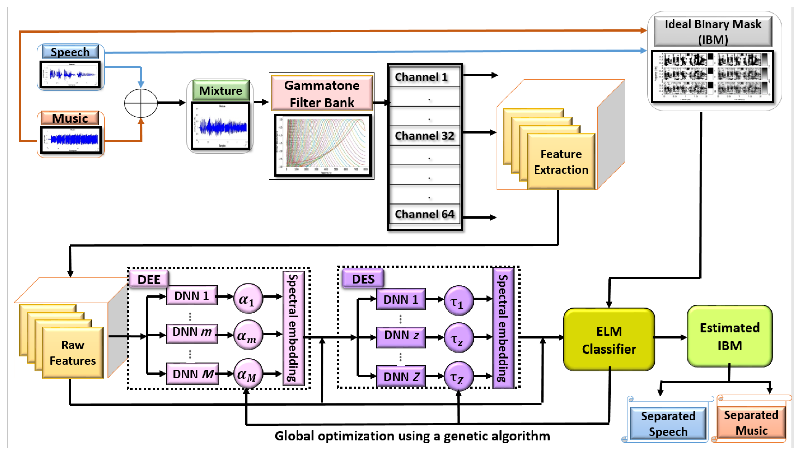
3. Overview of the System

The proposed system is depicted in Figure 1 and is divided into four phases: DNN training, multiview spectral embedding, ELM classification, and global optimization. To provide the training data, raw acoustic features were extracted from source signals. This was then used to train each DNN in each frequency channel individually. MVSE was then used to merge the penultimate layer’s learned features into a complementary features vector. The acquired features vector was then input into the second module, which extracted more robust and discriminative information, before classifying each TF unit into the speech domain or nonspeech domain with the ELM classifier. Finally, in order to optimize the parameters globally, a genetic approach was developed. The optimal ensemble system was used to classify each TF unit of the mixed signal in order to create binary masks (BM) for testing. By weighting the mixed cochleagram via the mask and correcting the phase shifts produced through Gammatone filtering, the predicted time-domain sources were resynthesized by applying the method described in [30].

The following is a description of the proposed framework’s architecture: On the equivalent rectangular bandwidth rate scale, the mixed signal with a sampling frequency of 16 kHz is put into a Gammatone filter bank with a 64 channel [31], with center frequencies evenly spread from 50 Hz to 8000 Hz. Each filter channel’s output is split into time frames with an overlap of 50% between successive frames.

A Gammatone filter bank is often used in single-channel audio separation tasks to model the cochlear filtering that occurs in the human ear. The cochlea in the inner ear contains thousands of hair cells that are sensitive to different frequencies of sound. These hair cells act as bandpass filters that decompose the incoming sound into its constituent frequency components. A Gammatone filter bank is a set of bandpass filters that are designed to mimic the frequency selectivity of the cochlear hair cells. The filters are based on the Gammatone function, which is a mathematical model of the impulse response of the auditory system. By applying a Gammatone filter bank to the mixed audio signal, we can decompose the signal into a set of frequency components that correspond to different regions of the cochlea [32].

This frequency decomposition can be useful in audio separation tasks because it allows us to isolate specific frequency components that correspond to different sources of sound. For example, if we are trying to separate a speech signal from a noisy background, we can use a Gammatone filter bank to isolate the frequency components that correspond to the speech signal and attenuate the components that correspond to the background noise. Overall, the Gammatone filter bank is a powerful tool for modeling the human auditory system and can be used to improve the performance of single-channel audio separation algorithms. The cochleagram [32] is formed by establishing the TF units of all the filter outputs. Then, we can classify each TF unit to its identical domain in order to estimate the BM, which is our aim.

However, the spectral characteristics of the source signals in various channels might be quite varied. As a result, we trained a subband classifier for each channel to make the decision. Because of its low computational complexity and high classification performance, we chose the ELM classifier [33,34,35,36]. For each TF unit, several features were extracted in order to conduct the classification. 15-Dimensions (15-D) of an Amplitude Modulation Spectrogram (AMS), 13-D of the Relative Spectral Transform and Perceptual Linear Prediction (RASTA-PLP), and 31-D of the Mel-Frequency Cepstral Coefficients (MFCCs) make up the feature set.

A features vector was created by concatenating the extracted features. We propose pooling many DNNs and establishing an ensemble system of DNNs to learn more discriminative and robust representations instead of sending the features vector straight into the classifier. Additionally, each individual DNN’s penultimate layer was embedded to investigate the complementary nature of the learned representation in order to increase the classification robustness, and as a result, the separation performance is also improved. At the top of the first module, a second module was stacked to extract more robust and discriminative representations for the classification. A genetic method was also created to identify the best coefficients for all DNNs and ELMs, resulting in more consistent estimates. We used the traditional frame-level acoustic feature extraction for each Gammatone filter channel’s output to gain the features of each TF unit, and the concatenated features vectors were used as the raw acoustic feature set, which was input into the DNN ensemble system.

The envelope of the mixture signal was calculated by using full-wave rectification and then decimated by a factor of four to generate the 15-D AMS. To create a 256-point Fast Fourier Transform (FFT), the decimated envelope was split into overlapping segments, and then Hanning windowing and zero padding were applied. To create the 15-D AMS [37], the FFT magnitudes were multiplied by uniformly spaced 15 triangular-shaped windows across the 15.6–400 Hz band. The spectral amplitude was compressed by using a static nonlinear transformation to create the 13-D RASTA-PLP. Each converted spectral component’s temporal trajectory was filtered and extended again, and then a traditional PLP analysis was performed [38,39]. A short-time Fourier transform with a Hamming window was used to obtain the 31-D MFCC, which was then warped to the Mel scale; after that, a log operation with a discrete cosine transform was used [40,41,42,43].

In addition, the delta features of the RASTA-PLP were also exploited to benefit the speech separation [38]. As a result, the original features of the RASTA-PLP were concatenated with their first- and second-order delta features (which are denoted by $▵\mathrm{and}▵▵$) to generate a combined features vector in order to learn features and classification. Finally, 85-dimensional raw acoustic features were produced from a collection of the following features: 15-D AMS, 13-D RASTA-PLP, 13-D $▵$ RASTA-PLP, 13-D $▵▵$ RASTA-PLP, and 31-D MFCC.

4. The Proposed Ensemble System Using DNN

Two modules with DNNs are introduced in this part. In the case of a mixed signal, the acoustic features are extracted for each TF unit in the cochleagram represented as ${\left\{x_n\right\}}_{n=1}^N$, where N is the number of frames.

4.1. DNN Ensemble Embedding (DEE)

Assume there are M DNNs in the DEE, where M is greater than one. An output layer, as well as a number of nonlinear hidden layers, are present in each DNN.

4.1.1. DNN Training

The m-th DNN learns a mapping function that can be expressed as in Equation (1).

$$F_m=f_m\left(w_{m\Xi }{g}_{m(\Xi -1)}\right(\dots w_{m\xi }{g}_{m(\xi -1)}(\dots w_{m2}{g}_{m1}(w_{m1}\left\{{\left(x_n\right)}_{n=1}^N\right\}\left)\right)\left)\right)$$

(1)

where $\xi =1,\dots ,\Xi$ indicates the number of hidden layers; $w_{m\xi }$ is the weight linking the $\xi$-th hidden layer and the one above it; $fm(·)$ indicates the output activation function; and $g_{m\xi }(·)$ indicates the activation function of the $\xi$th hidden layer.

The activation function that we chose is the sigmoid function. It is worth noting that each DNN in the same module had a different weight parameter $W={\left\{w_m\right\}}_{m=1}^M$. The network was pretrained by utilizing the Restricted Boltzmann Machine (RBM) in a greedy layer-wise style, followed by back-propagation finetuning. We used the raw acoustic features that were extracted as the training data. The Gaussian–Bernoulli RBM (GBRBM) was used to train the first layer, and its energy function can be defined as

$$E_{GBRBM}(v,h)=\sum _{\varphi \in vis}^{}\frac{{(v_{\varphi }-b_{\varphi })}^2}{2{\sigma }_{\varphi }^2}-\sum _{v\in hid}^{}{c}_v{h}_v-\sum _{\varphi ,v}^{}{w}_{\varphi v}{h}_v\frac{v_{\varphi }}{{\sigma }_{\varphi }}$$

(2)

where $h_v$ and $v_{\varphi }$ are both vth and $\varphi$th units of the hidden layer and visible layer, respectively; $c_v$ denotes the bias of the vth hidden unit; $b_{\varphi }$ denotes the bias of the $\varphi$th visible unit and the weight between the $\varphi$th visible units; and the vth hidden unit is $w_{\varphi v}$. For all the remaining layers, Bernoulli–Bernoulli RMBs are used:

$$E_{GBRBM}(v,h)=\sum _{\varphi \in vis}^{}{b}_{\varphi }{v}_{\varphi }-\sum _{v\in hid}^{}{c}_v{h}_v-\sum _{\varphi ,v}^{}{w}_{\varphi v}{h}_v{v}_{\varphi }$$

(3)

The RBM is a generative model in which the parameters are improved by using a stochastic gradient descent on the training data’s log likelihood [44].

$$\frac{\partial logp\left(v\right)}{\partial w_{ij}}\approx {〈v_i{h}_j〉}_{x^0}-{〈v_i{h}_j〉}_{x^{\infty }}$$

(4)

where $〈·〉$ indicates the expected outcomes under the distribution provided by the following subscript. $x^{\infty }$ denotes the equilibrium distribution defined by the RBM while $x^0$ indicates the distribution of the data. The DNN is initialized by using the learned parameters from a stack of RBMs. This empirical approach of initialization has been created to assist the subsequent backpropagation finetuning, and it is often crucial when training a deep network with numerous hidden layers [45]. Finally, the back-propagation method is used to finetune the whole network. After the network has been adequately finetuned, the penultimate layer activations represented as $P_m$ are regarded as the learned intermediate representations instead of the final layer activations of the DNN [46,47,48,49].

4.1.2. Spectral Embedding in Multiple Views

In M DNNs, the learned intermediate representations $P={\{P_m\in \Re {}^{d_m\times n}\}}_{m=1}^M$ are fed into a Laplacian multispectral graph to investigate the complimentary characteristics [4]. Varying representations have different strengths, which might lead to different mistakes in the separation system [5].

MVSE is a technique used to take advantage of complementary representations and exploit the strengths of specific representations. Assume that $P=[P_{m1},P_{m2},\dots ,P_{mn}]\Re {}^{d_m\times n}\}$ is the m-th learned representation, and consider $p_{mj}$ as an arbitrary point and that its k associated points are in the same features set (for example, nearest neighbors) $p_{mj1},p_{mj2},\dots ,p_{mjk}$; the patch of $p_{mj}$ is defined as $P_{mj}=[p_{mj},p_{mj1},p_{mj2},\dots ,p_{mjk}]\in \Re {}^{d_m\times (k+1)}$, where v represents the dimension of the intended embedding and is a predetermined number. The component optimization for the jth patch on the mth feature set is used in the projected low-dimensional space to preserve the locality. This part is

$$\underset{R_{mj}}{arg\; min}\sum _{i=1}^k{\parallel r_{mj}-r_{mji}\parallel }^2{\left({\mu }_{mj}\right)}_i$$

(5)

where ${\mu }_{mj}$ is a column vector that has a k-dimension and is weighted by ${\left(u_{mj}\right)}_i=(ex{p}^{-\parallel p_{mj}-p_{mji}\parallel }{}^2/\gamma )$, and the width of the neighborhoods is controlled by $\gamma$; as a result, we can reformulate the part optimization to

$$\underset{R_{mj}}{arg\; min}tr(\left[\begin{array}{c}(r_{mj}-r_{mj1})\\ \cdots \\ (r_{mj}-r_{mjk})\end{array}\right]\times [r_{mj}-r_{mj1,}·,r_{mj}-r_{mjk}]diag\left({\mu }_{mj}\right))=\underset{R_{mj}}{arg\; min}tr\left(r_{mj}{L}_{mj}{\left(R_{mj}\right)}^T\right)$$

(6)

where the trace operator is $tr(·)$ and $L_{mj}=\left[\begin{array}{cc}{\sum }_{i=1}^k{\left({\mu }_{mj}\right)}_i& -{\left({\mu }_{mj}\right)}^T\\ -{\mu }_{mj}& diag\left({\mu }_{mj}\right)\end{array}\right]\in {\Re }^{(k+1)\times (k+1)}$ encodes the jth patch’s objective function on the mth learned representation.

A suitably smooth, low-dimensional-embedding R mj can be constructed by maintaining the inherent structure of the jth patch on the mth learned representation. The DNN ensemble extracts multiple features with varying mapping parameters that may contribute differently to the final low-dimensional embedding. A collection of non-negative weights $\alpha =[{\alpha }_1,\cdots ,{\alpha }_m]$ is imposed on the portion optimizations of various DNNs independently to investigate the complementary characteristics of different extracted features. The $P_{mj}$ plays a more important role in learning how to obtain the low dimensional embedding $R_{mj}$ as ${\alpha }_m$ grows larger. The component optimization for the jth patch is represented as the sum of all the m-th learned representations and can be formulated as

$$\underset{R_J={\left\{R_{mj}\right\}}_{m=1}^M,\alpha }{arg\; min}\sum _{m=1}^M{\alpha }_{m}tr\left(R_{mj}{L}_{mj}{\left(R_{mj}\right)}^T\right)$$

(7)

There is a low-dimensional embedding $R_{mj}$ for each patch $P_{mj}$. By supposing that the coordinate for $R_{mj}=\left[\begin{array}{c}{r}_{mj},r_{mj1},r_{mj2},\cdots ,r_{mjk}\end{array}\right]$ is chosen from the global coordinate $R=\left[\begin{array}{c}{r}_1,r_2,r_3,\cdots ,r_n\end{array}\right]$, all $R_{mj}$ can be integrated as one, i.e., $R_{mj}=R{V}_{mj}$, where $V_{mj}\in {\Re }^{n\times (k+1)}$ is the matrix employed in a patch in the original high-dimensional space to encode the spatial relation of the samples. Consequently, Equation (7) can be rewritten as

$$\underset{R_J,\alpha }{arg\; min}\sum _M^{m=1}{\alpha }_{m}tr(R{V}_{mj}{L}_{mj}{\left(V_{mj}\right)}^T{\left(R\right)}^T$$

(8)

The global coordinate alignment is calculated by adding all the optimization parts together and is expressed as

$$\left\{\begin{array}{c}{arg\; min}_{R,\alpha }\sum _M^{m=1}{\alpha }_m^{ϵ}tr\left(R{L}_m{R}^T\right)\hfill \\ s.t.R{R}^T=I,\sum _M^{m=1}{\alpha }_m^{ϵ}=1,{\alpha }_m\ge 0\hfill \end{array}\right.$$

(9)

where the alignment matrix for the mth learned representations is $L_m\in {\Re }^{n\times n}$, and it is also defined as $L_m={\sum }_{j=1}^N{V}_{mj}{L}_{mj}{\left(V_{mj}\right)}^T$. The restriction $R{R}^T=I$ is used to determine R in a unique way. The coefficient for managing the interdependency between various perspectives is the Exponent $ϵ$, which should satisfy $ϵ\ge 1$. We constructed a symmetric and positive semidefinite normalized graph Laplacian $L_{sys}$ by conducting a normalization on $L_m$. $L_{sys}$ is defined as

$$L_{sys}={D_m}^{-\frac{1}{2}}{L}_m{D_m}^{-\frac{1}{2}}=I-{D_m}^{-\frac{1}{2}}{Q}_m{D_m}^{-\frac{1}{2}}$$

(10)

where $Q_m={\Re }^{n\times n}$ and ${\left[\begin{array}{c}{Q}_m\end{array}\right]}_{ij}=exp(-\Vert p_{mi}-p_{mj}{\Vert }^2/\gamma )$ if $p_{mi}$ is one of the $p_{mj}$’s k-nearest neighbors or vice versa; $L(\alpha ,\lambda )={\sum }_{m=1}^M{\alpha }_m^{\epsilon }tr\left(R{L}_{sys}{R}^T\right)-\lambda \left({\sum }_{m=1}^M{\alpha }_m-1\right)$ otherwise. $D_m$ is a diagonal matrix with the degrees ${\left[\begin{array}{c}{D}_m\end{array}\right]}_{jj}={\sum }_l{\left[\begin{array}{c}{Q}_m\end{array}\right]}_{jl}$, and it is called a degree matrix.

Equation (9) is a nonconvex nonlinear optimization problem with nonlinear constraints, and the best solution can be found by using an iterative technique such as the Expectation Maximization (EM) technique [50]. Both R and $\alpha$ are updated iteratively in an alternating style by the optimizer.

Step 1: Fix R to update $\alpha$

By using a Lagrange multiplier $\lambda$ and taking into account the restriction ${\sum }_{m=1}^M{\alpha }_m^{ϵ}=1$, the Lagrange function can be written as

$$L(\alpha ,\lambda )=\sum _{m=1}^M{\alpha }_m^{\epsilon }tr\left(R{L}_{sys}{R}^T\right)-\lambda \left(\sum _{m=1}^M{\alpha }_m-1\right)$$

(11)

The solution for ${\alpha }_m$ can be obtained by

$${\alpha }_m=\frac{{\left(1/tr\left(R{L}_{sys}{R}^T\right)\right)}^{1/(\epsilon -1)}}{{\sum }_{m=1}^M{\left(1/tr\left(R{L}_{sys}{R}^T\right)\right)}^{1/(\epsilon -1)}}$$

(12)

When R is fixed, then Equation (12) gives the global optimal $\alpha$.

Step 2: Fix $\alpha$ to update R

The optimization problem in Equation (9) is equivalent to

$$\underset{R}{min}\left(RL{R}^T\right)s.t.R.R^T=I$$

(13)

where $L={\sum }_{m=1}^M{\alpha }_m^{ϵ}{L}_{sys}$. When $\alpha$ is fixed, Equation (9) has a global optimum solution according to the Ky-Fan theorem [51]. The optimal R is given as the eigenvectors related to the lowest d eigenvalues of the L matrix. After obtaining the embedded feature R, then the raw acoustic features will be concatenated with it to produce a new feature vector, as the raw acoustic features can offer global information that can aid in mask estimation. The updated feature vector will be sent into the ensemble stacking in the second module.

4.1.3. DNN Ensemble Stacking (DES)

A second DNN ensemble is stacked on top of the first in this module. The first DNN ensemble is considered a lower module, whereas the second ensemble is considered a higher module. As input to the upper module, the embedded features of the lower module with the raw features are concatenated. This enables the extraction of higher-order and more robust discriminative features. DES is a masking-based module, unlike the previous module, in which DNNs are trained by using pretraining, and then supervised finetuning is applied. In order to learn feature encoding, DES includes training $Z>1$ DNNs, which is indicated as ${\varphi }_Z$ at this stage. The z-th DNN’s learning procedure can be represented as

$${\varphi }_z=f_z\left(g_{zI}(\cdots g_{z1}\left(\sigma \right))\right),z=1,2,\cdots ,Z$$

(14)

where $\varphi$ is the result of concatenating the embedded and raw acoustic features of the lower module. In DES, each single DNN learns a masking function. In the output layer, linear, softmax, and sigmoid functions are common activation functions. We selected the softmax function for the output layer because the training objective was the IBM, which has a value of either 0 or 1, and the softmax function is an extension of the logistic function, whose output reflects a categorical distribution:

$$p(y=j\mid x)=\frac{e^{x^{\mathrm{T}}{w}_j}}{{\sum }_{k=1}^K{e}^{x^{\mathrm{T}}{w}_k}}$$

(15)

where $p(y=j\mid x)$ indicates the predicted probability for the jth class given a sample vector x and a weighting vector w. The combined features set is utilized as training data for the first GBRBM, whose hidden activations are subsequently used as new training data for the second RBM and so on. To obtain the internal discriminative representations, the pretrained GBEBM, RBMs, and softmax layer are merged and finetuned with labeled data. The softmax classifier is trained during the first 10 iterations of the module while it is being finetuned. The outputs of the DES’s penultimate layer are then sent into a multispectral graph Laplacian to investigate the complementary property once the network has been finetuned. In the following stage, ELM is used to classify the concatenation for both the embedded features with raw features.

4.1.4. ELM-Based Classification

We utilized ELM [33] to classify the TF units into the target domain or interference domain at this step by using the concatenated features. For a single-layer feed-forward neural network, ELM is suggested. With K hidden nodes, the ELM model may be written as

$$t_{\varphi }=\sum _{k=1}^{K}S(x_{\varphi },u_k,v_k){\beta }_k,\varphi =1,\cdots ,\Phi$$

(16)

where $x_{\varphi }$ is the input vector and $t_{\varphi }$ denotes the output. The parameters of the activation function of the kth hidden node are $u_k$ and $v_k$, and the output of the kth hidden node with respect to the kth input is $S(x_{\varphi },u_k,v_k)$. The output weight of the kth hidden node is ${\beta }_k$. The Equation (16) can be formulated as

$$T=S\beta$$

(17)

where $T={\left[\begin{array}{c}{t}_1,\cdots ,t_{\Phi }\end{array}\right]}^T$, $\beta ={\left[\begin{array}{c}{\beta }_1,\cdots ,{\beta }_K\end{array}\right]}^T$, and the hidden output matrix S can be written as

$$\mathit{S}={\left[\begin{array}{ccc}s\left(x_1,u_1,v_1\right)& \cdots & s\left(x_1,u_K,v_K\right)\\ ⋮& \ddots & ⋮\\ s\left(x_{\Phi },u_1,v_1\right)& \cdots & s\left(x_{\Phi },u_K,v_K\right)\end{array}\right]}_{\Phi \times K}$$

(18)

The parameters are learned in two phases by using an ELM: random feature mapping and linear parameter solution. By using the activation function $s\left(·\right)$ with randomly initialized parameters, the input data are projected into a feature space in the first step.

The ability of the randomly initialized parameters to approximate any continue function has been demonstrated [33,36]. As a consequence, the output weight $\beta$ is the lone parameter that has to be computed, which can be estimated by using the following formula:

$$\widehat{\beta }=S^{♠}T$$

(19)

where $S^{♠}$ is the Moore–Penrose generalized inverse.

4.1.5. Global Optimization with a Genetic Algorithm

The last stage in this research involved using a genetic algorithm to optimize the weights $\alpha =\left[\begin{array}{c}{\alpha }_1,\cdots ,{\alpha }_M\end{array}\right]$ and $\tau =\left[\begin{array}{c}{\tau }_1,\cdots ,{\tau }_Z\end{array}\right]$ globally based on the estimation error, as shown in Figure 1. Essentially, a genetic algorithm includes a population containing a certain number of people. Every individual in a population has the potential to solve the optimization problem. As a result, a new generation is created by the use of selection, crossover, and mutation among individuals. This procedure is performed numerous times until a new individual offers the best solution to the problem. Based on our research, the generated DNN ensemble and stacking system were finetuned by employing genetic algorithms in the next steps:

(i)

Defining the fitness function

The developed genetic algorithm’s fitness function in this step was to reduce the mean square error between the real TF unit value T and the estimated value $S\widehat{\beta }$:

$$\left\{\begin{array}{cc}arg\; min\hfill & \frac{1}{N}\sum _N{\left(T-S\widehat{\beta }\right)}^2\hfill \\ {\left\{{\alpha }_m\right\}}_{m=1}^M,{\left\{{\tau }_z\right\}}_{z=1}^Z\hfill \\ \\ s.t.\sum _{m=1}^M{\alpha }_m^{\epsilon }=1,\hfill & {\alpha }_m\ge 0\hfill \\ \\ \sum _{z=1}^Z{\tau }_z^{\epsilon }=1,\hfill & {\tau }_z\ge 0\hfill \end{array}\right.$$

(20)

(ii)

Determining the initial population of chromosomes $L_0$

For both steps, the initial population size was selected as 1000 chromosomes (individuals) for this genetic algorithm. These initial chromosomes represent the first generation.

(iii)

Encoding

Each chromosome in the population was encoded by using binary strings of 0 s and 1 s. Every ${\alpha }_m$ was represented as a 10-bit string of binary numbers (0 s and 1 s) in the DEE step. Similarly, each chromosome (individual) refers to Z weights in the DES step. As a consequence, each chromosome was represented by $Z\times 10$ bit strings.

(iv)

Boundary conditions

The boundary conditions were set in both stages such that every element ${\left\{{\alpha }_m\right\}}_{m=1}^M,{\left\{{\tau }_z\right\}}_{z=1}^Z$ had a positive value.

(v)

Reproduction of next generations $\left(L_1,L_2,L_3,\cdots \right)$

The fitness function was used to test each chromosome in the first generation ($L_0$) to calculate how effectively it solved the optimization issue. The chromosomes that performed better or were more fit were passed on to the next generations. They were wiped out otherwise. Crossover occurred when two chromosomes swapped some bits of the same region to produce two offspring, whereas mutation occurred when the bits in the chromosome were turned over (0 to 1 and vice versa). The occurrence of mutation was determined by the algorithm’s mutation probability ($\rho$) as well as a random number generated by the computer ($\omega$). We set the $\rho$ value to $0.005$ in this stage. The mutation operator can be defined as follows:

$$mutation=\left\{\begin{array}{cc}1\left(occurs\right)\hfill & \rho \ge \omega \hfill \\ 0\left(notoccur\right)\hfill & \rho <\omega \hfill \end{array}\right.$$

(21)

(vi)

Until the best chromosome was attained, the processes of selection, crossover, and mutation were repeated.

Finally, with regard to the input data, a binary mask was created, and by weighting the mixture cochleagram, the estimated time-domain sources were resynthesized by using the mask.

5. Experimental Results and Discussion

The proposed separation technique is evaluated with recorded audio signals in this section. The simulation was achieved by using the MATLAB codes that were running on a PC with an Intel Core i5 processor running at 3.20 GHz and 8 GB of RAM. We used voice data from the ‘CHiME’ database [52], which has data from 34 speakers, and each speaker has 500 utterances. For the training data, ten utterances were chosen at random and mixed with music [53] at 0 dB. The test set was made up of 25 different utterances from the same speaker’s training data mixed with the same music at 0 dB. Unless otherwise specified, we used data from the same speaker for both training and testing, i.e., a speaker-dependent setup. We started by extracting each channel’s basic acoustic features. Then, before being fed into the system, we applied normalization to the extracted features until we achieved a mean and unit variance of zero [54]. As the first layer, the GBRBM was trained between the visible layer and the first hidden layer for each DNN in the system, whereas the higher layers were built by using RBM pretraining data. For pretraining, we used 50 epochs of gradient descent, and to finetune the whole network, we used 50 epochs of gradient descent. The GBRBM’s learning rate was set to 0.001, whereas RBM’s learning rate was set to 0.01. The first 5 epochs’ momentum was set to 0.5, while the rest of the epochs’ momentum was set to 0.9. A somewhat modest DNN with two hidden layers was used because of its performance and computational complexity. The small number of adjustable network parameters allows for fast, scalable training with a satisfactory performance. The size of the nearest neighbors in the MVSE was set to be 10. The embedded feature dimension was set at 50. When training the ELM classifier, the embedded features were always mixed with raw acoustic features. The proposed system was compared with different machine learning approaches, such as Support Vector Machine (SVM)-based, ELM-based, DNN-based, and DNN-ELM-based approaches.

The fusion technique was exploited via concatenation to merge the raw acoustic features with their first and second delta features, which were used to train the SVM and ELM for the SVM-based and ELM-based techniques. A total of 50 epochs were used for both minibatch gradient descents for the RBM pretraining and for network finetuning to train the DNN-based approach. The output of the DNN’s final hidden layer was used to train an ELM by using DNN-ELM-based approaches. By using the raw acoustic features of each TF unit, all four approaches were used to train a classifier for each channel. In addition, as a comparison approach, we used the Itakura–Saito NMF (IS-NMF) [5] and NMF2D [32] algorithms. IS-NMF has already been proven to accurately capture the semantics of audio and to be more appropriate for representation than the regular NMF [55]. MGD IS-NMF-2D [32], which was recently presented, delivers promising separation results for music mixtures and is regarded as a competitive solution to solving separation difficulties, where MGD is the Multiplicative Gradient Descent (MGD).

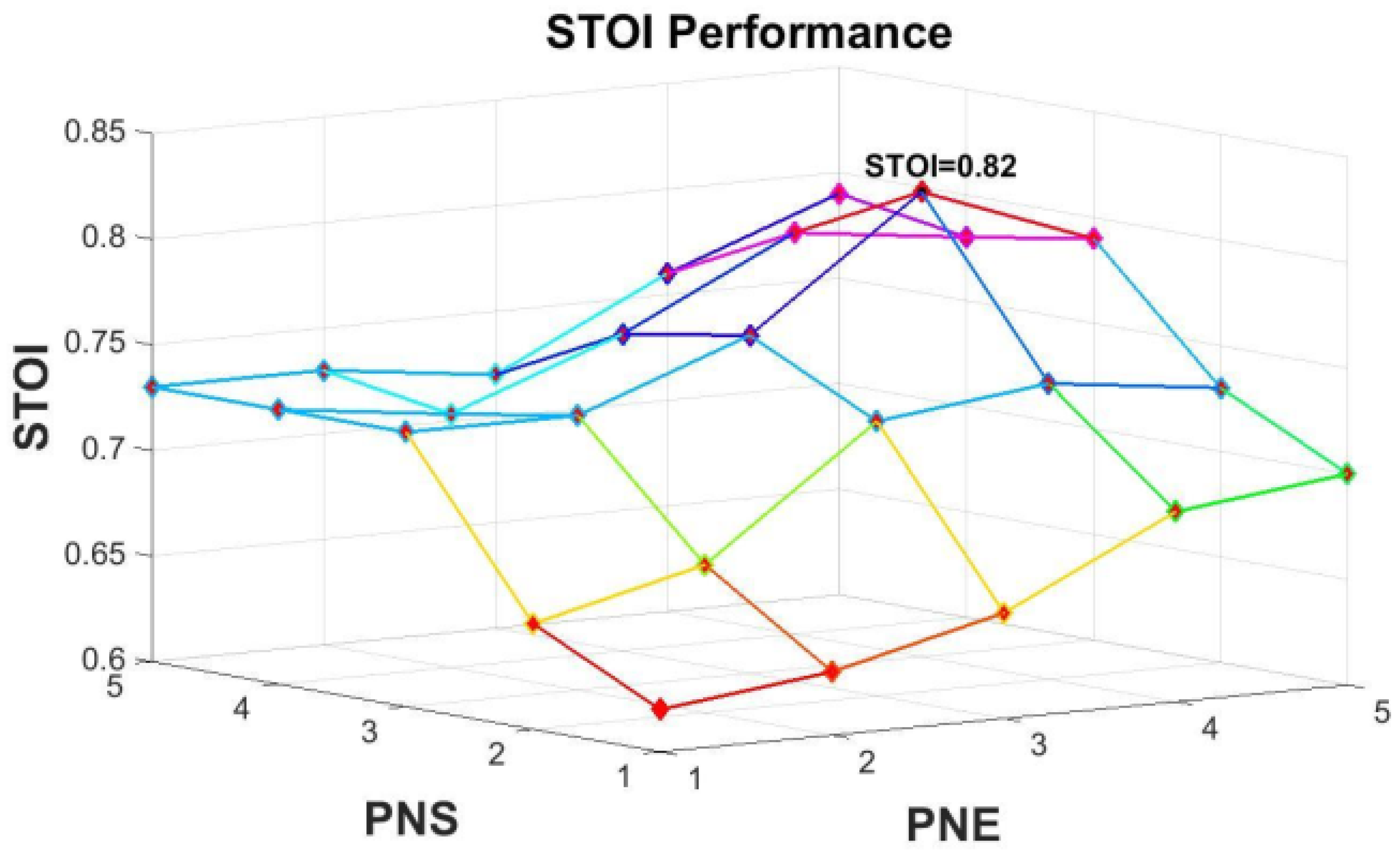
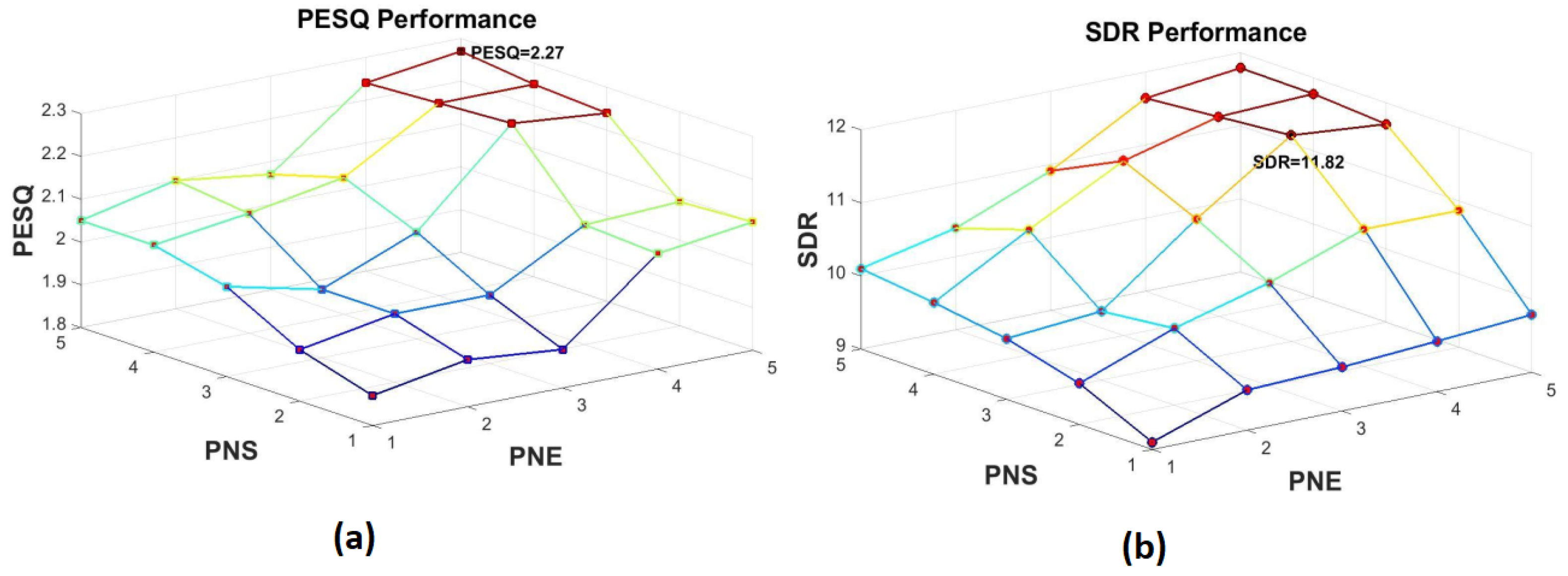
5.1. Optimizing the Number of DNNs

The ensemble of DNNs is the initial module. We compared the separation performance according to the number of DNNs to calculate the number of DNNs in each module. We initially evaluated the separation performance for the set 1 DNN in DEE and DES (referred to as 1DEE-1DES). Then, we evaluated the performance of the set 2 DNNs in DES and 1 DNN in DEE (2DES-1DEE). The experiments were carried out until all the settings (5DEE-5DES) were evaluated. Figure 2 depicts the separation findings. In the trials, we trained a different number of DNNs by using the same training data. The Short-Time Objective Intelligibility (STOI) [56] is an evaluation metric that is used to evaluate the Objective Speech Intelligibility (OSI) of time-domain signals. The STOI scores are closely associated with speech intelligibility scores, according to empirical evidence. The expected intelligibility improves as the STOI value rises. Adding a second DNN in DEE and DES increases the separation performance over employing a single DNN in each module, as seen in Figure 2. When one DNN is added to each module, the performance increases dramatically when compared to when only one DNN is used in each module. Not only that, but after adding the DNNs, it was observed that the improvement became more significant. With more DNNs in the DES module, this is amplified even further. With 4 DNNS and 3 DNNs from the first and second modules, respectively, the greatest attainable STOI is 0.82. However, with five DNNs or more, the improvement in the separation performance becomes less significant. This might be because more DNNs cannot extract additional discriminative features that would increase the separation performance. We employed various metrics to evaluate the proposed learning system, such as a Perceptual Evaluation of Speech Quality (PESQ) and Signal-to-Distortion Ratio (SDR), to further study the usefulness of the number of DNNs in the learning system.

Figure 3a,b depicts the results. The separation performance when the 4DEE-3DES was used improved when compared to when the 4DEE-2DES and 3DEE-3DES were used, as shown in Figure 3a. Although 5DEE-5DES had the greatest PESQ, the improvement was less substantial when compared to 4DEE-3DES. Figure 3b shows that the separation performance of 4DEE-3DES was 11.82 dB, which was much superior to the performance of a single DNN in each network module. To summarize, the separation performance improved as the number of DNNs in each module increased; however, the improvement was less noticeable after 4 DNNs were in each module, which means that using 4 DNNs in DEE and 3 DNNs in DES is a decent decision given the computational complexity of the network.

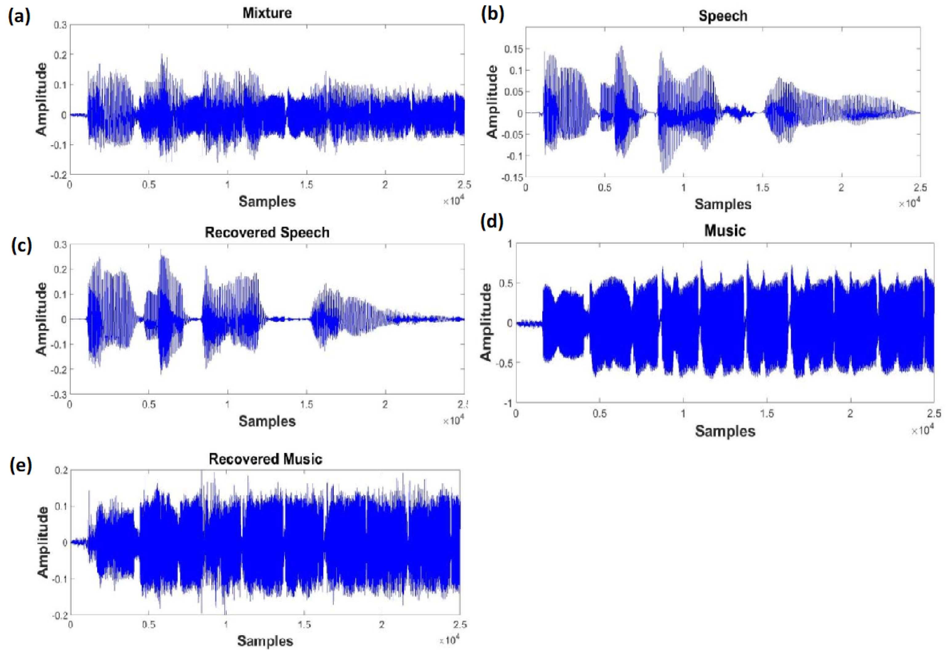
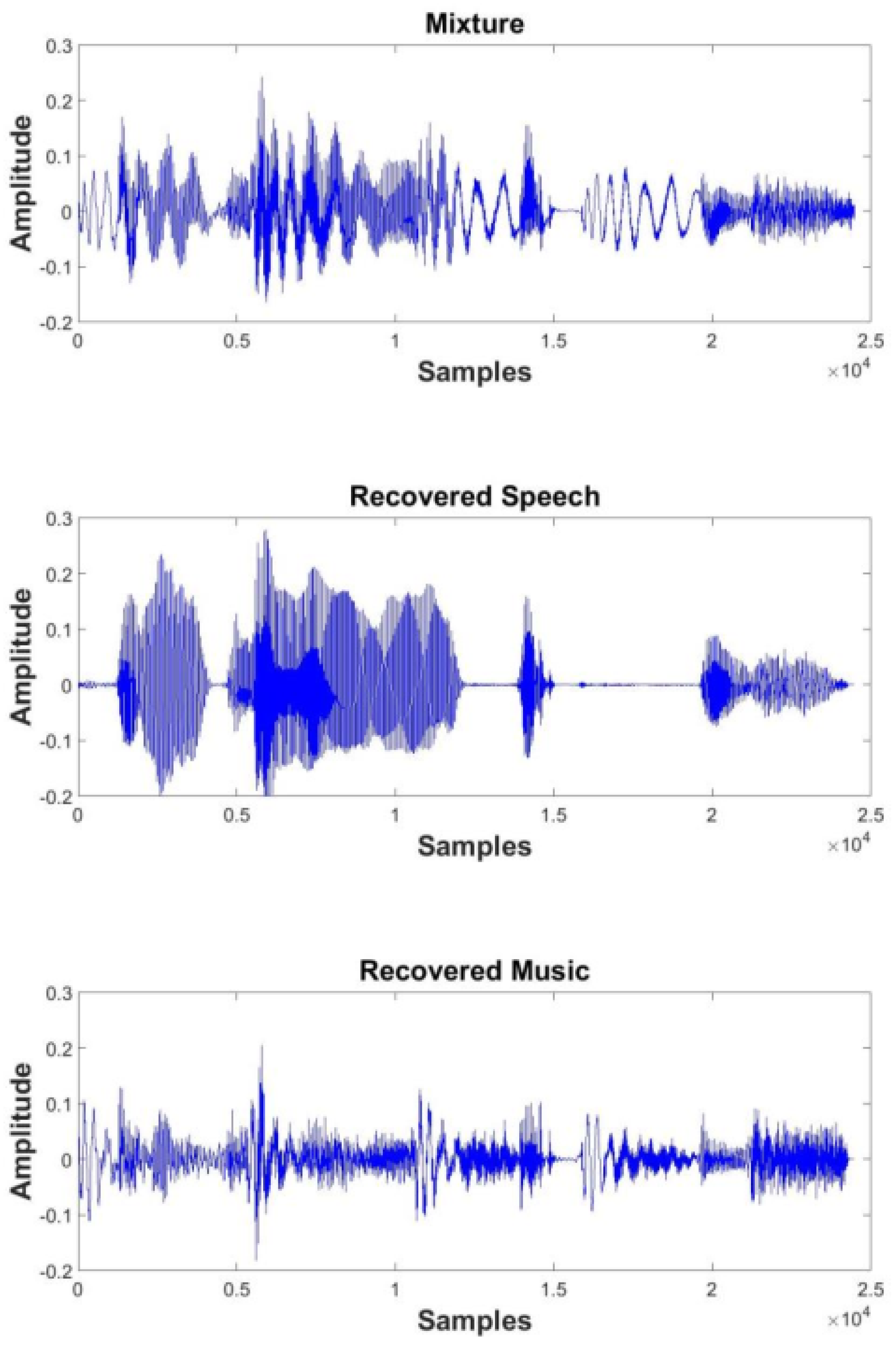
5.2. Speech Separation Performance

We compared the separation performance of our proposed strategy with the performance of selected approaches for various mixtures in order to demonstrate its effectiveness. A total of 10 utterances were selected randomly from males and females to create the training set. At 0 dB, the selected utterances from the SNR training data were mixed with guitar and bass music. For the testing data, 30 utterances were created differently than the training data mixed with guitar and bass music at 0 dB SNR in order to test our system. From each TF unit, a feature set of 85 dimensions (85-D) was extracted from the training and testing data for preprocessing. In this experiment, the Signal-to-Distortion Ratio (SDR), which includes the Signal-to-Interference Ratio (SIR) and Signal-to-Artifacts Ratio (SAR), was used to evaluate the separation performance. The following methods were selected for comparison: Itakura–Saito Non-Negative Matrix Factorization (IS-NMF), Non-Negative Two-Dimensional Matrix Factorization (NMF2D) based on an Extreme Learning Machine (ELM) and based on a deep neural network (DNN), and Ideal Binary Mask (IBM). The IS-NMF was used in conjunction with a clustering approach, whereby the mixed signal was factorized into $\aleph =2,4,\cdots ,10$ components and then the ℵ components were clustered to each source by using a grouping method. For comparison, the best value of the outcome of each case of the ℵ different configurations was kept. The mixed signal spectral and temporal features were factorized in the nonuniform TF domain created by the Gammatone filter bank for MGD IS-NMF-2D, where the MGD is the Multiplicative Gradient Descent. To separate the mixed signal, the obtained features were employed to produce a binary mask. The mask was produced directly from the speech and music by using the IBM technique. According to Figure 4, the SDR performance varied significantly depending on the separation approaches used. The ELM-based technique had an average SDR of 7.47 dB for the mixtures, whereas the NMF-2D method had an average SDR of 8.37 dB, and the DNN delivered an average SDR of 9.83 dB. However, our proposed method had an average SDR of 11.09 dB, and the IBM had an average SDR of 12.66 dB. It is worth noting that the DNN-based techniques and our proposed system’s outcomes outperformed the ELM-based approach. This is attributed to the deep architecture’s classified features, which are more discriminative than shallow networks. It is also worth noting that both the DNN and the proposed system had a high SDR performance. Furthermore, the proposed technique consistently outperformed the DNN in terms of the performance. This supports our findings that the proposed system can extract more complementary features than a single DNN. It also demonstrated that the higher layers of deep architecture represent more abstract and discriminative features than the lower ones.

To further analyze the separation performance of the proposed approach, an experiment was conducted with a mixture of a female voices mixed with guitar music at 0 dB. Figure 5 depicts the original speech, music, mixture, and separation results. The speech had an SDR of 11.69 dB, whereas the music had an SDR of 9.16 dB.

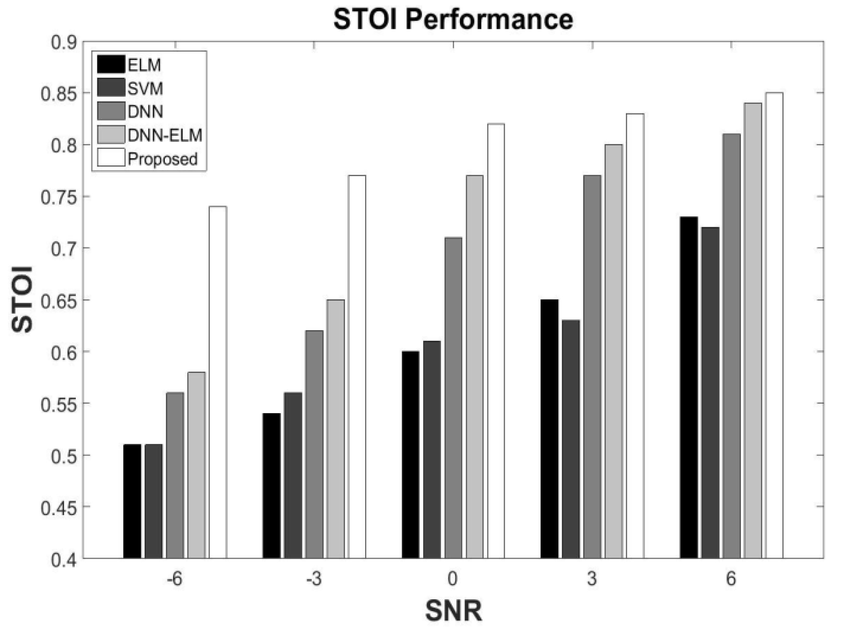
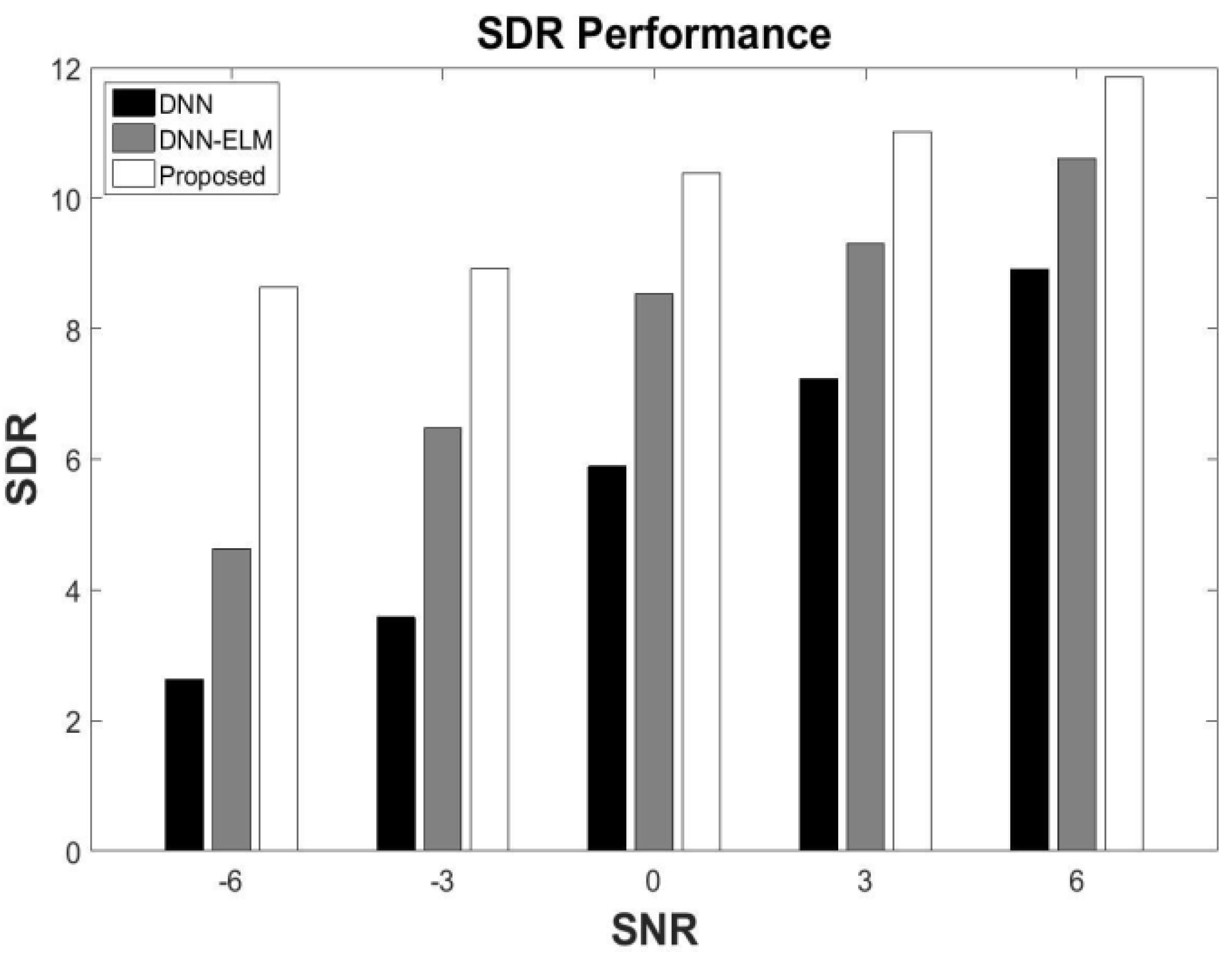
5.3. Generalization under Different SNR

This section describes the experiments that were performed to evaluate the effectiveness of the proposed method under different SNR conditions. The training set comprised mixtures at a single input SNR, and the system was evaluated on mixtures with various SNRs to generalize the SNR. To create the test data, 10 utterances of a speaker were chosen and mixed with the music at 0 dB SNR, whereas 20 utterances of the same speaker were chosen and combined with the same music at SNRs ranging from −6 dB to 6 dB with a 3 dB increase. ELM-based, SVM-based, DNN-based, and DNN-ELM-based algorithms were selected for comparison purposes. Figure 6 shows a comparison of several separation approaches in terms of the output of the Short-Time Objective Intelligibility (STOI). There were several observations to consider. Originally, deep architectures such as DNN, DNN-ELM, and the proposed technique significantly outperformed shallow architectures such as the ELM and SVM across a wide range of input SNRs. When compared to ELM, the proposed technique resulted in an average STOI improvement close to 24%. The proposed technique achieved a 29% improvement, especially at −6 SNR. This was due to the ability of deep architecture to extract the features by using a multilayer distributed feature representation, with higher levels representing more abstract and discriminative features. As a result, the Binary Mask (BM) created by deep architectures was more precise than those generated by shallow architectures. In addition, DNN-ELM produced higher SNR results than the DNN. This was because of the assistance of the ELM classifier. Although the outputs of the DNN already created an estimated BM, the ELM could produce additional features extracted from the DNN outputs and categorize them to their corresponding domain with a higher accuracy. Finally, among the deep architectures, the proposed technique produced the best STOI result. It is also worth noting that the separation performance was not affected dramatically by the SNR. The proposed approach showed increased robustness when compared to other techniques, as the STOI index changed relatively slightly because DNN ensembles with multiview spectral embedding can extract more beneficial complementary and robust features. In addition, the embedded features in the stacking module were more discriminative than in the lower module. Moreover, the genetic algorithm was utilized to globally improve the parameters in order to obtain a higher level of classification accuracy. The SDR performance was plotted in order to further analyze the effectiveness of the proposed technique. To compare, we used deep architectures to learn and categorize the input signals, including the DNN and DNN-ELM.

Figure 7 depicts the findings of the comparison and shows that our proposed method outperformed the DNN and DNN-ELM over a wide range of input SNRs. The ability of the proposed approach to extract more discriminative features than a single DNN was demonstrated.

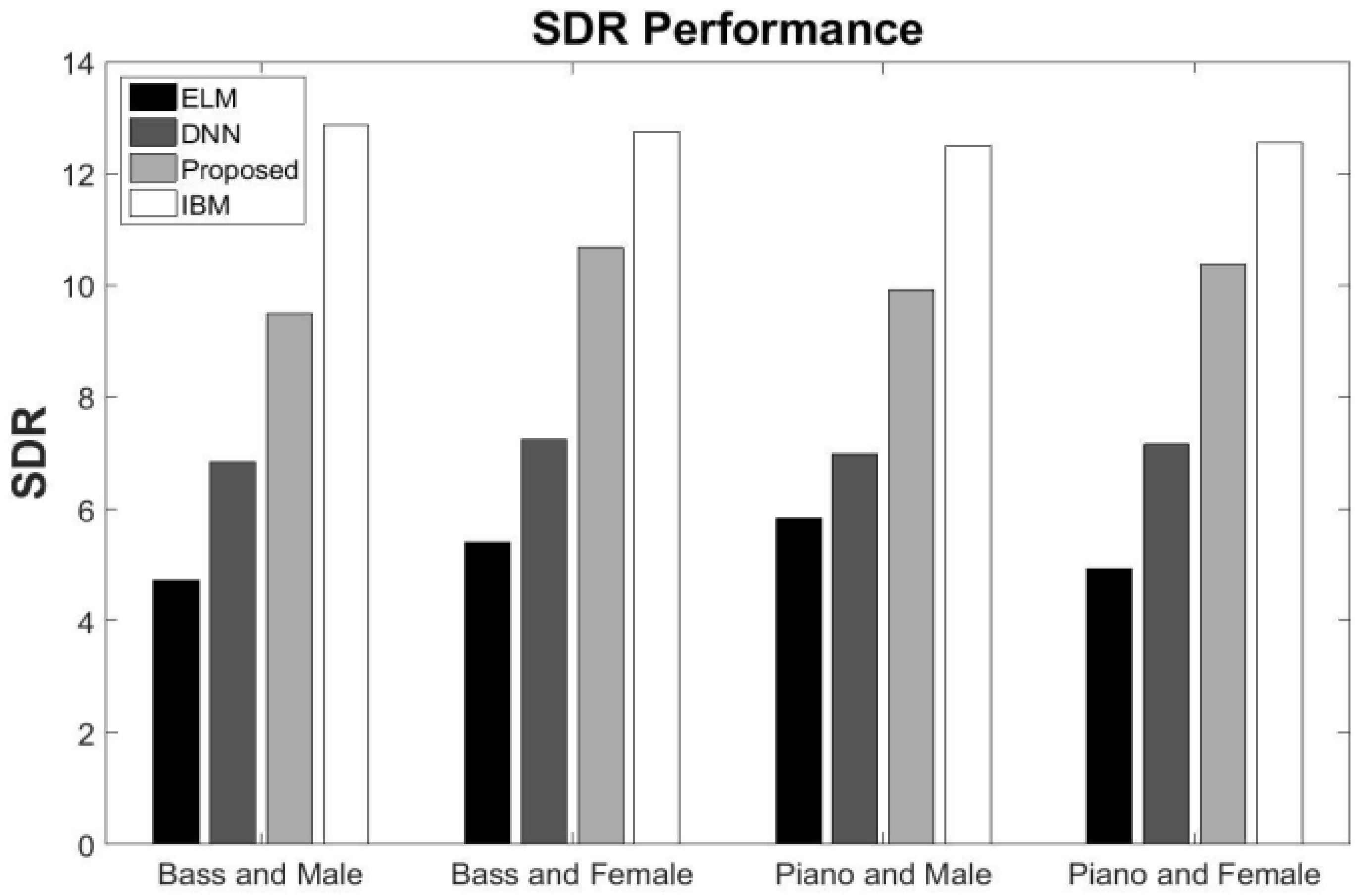
5.4. Generalization to Different Input Music

We conducted tests to show the generalization capabilities of our proposed system. In the testing set, the interfering music differed from that in the training set, but the testing speech (which differed from the training speech) was from the same speaker. The system was evaluated by using a blend of speech and unseen music, whereby the training set included signals mixed with a piece of music at 0 dB. To train the proposed system, we randomly selected 10 male and female utterances from the ‘CHiME’ dataset and mixed them with guitar music at 0 dB SNR in order to produce the training set. The features set included 85-D raw acoustic features. To evaluate our system, 30 male and female utterances that were different from those in the training data were selected and mixed with bass and piano music at 0 dB. During the preprocessing, for each TF unit, the feature set with 85-D of the testing data was extracted and then normalized to a mean and unit covariance of zero. The ELM-based, DNN-based, and IBM approaches were selected for comparison. Figure 8 depicts the comparative result. First, despite the fact that the proposed approach was trained with the selected music, its applicability to different music mixtures resulted in a good performance, as shown in Figure 8. The bass and female mixture’s SDR performance was 10.67 dB. It should also be highlighted that the proposed technique outperformed the ELM-based method substantially. The reason for this is that the deep architecture could extract more separable features, which increased the classification accuracy when estimating the binary mask. The proposed approach also outperformed the DNN-based technique, which implied that the DNN ensembles and stacking could give more comprehensive information than a single network. Although the IBM approach produced the highest overall outcomes, the proposed technique produced results that were almost as good as the IBM method. In terms of the SDR performance, the proposed technique achieved 10.12 dB, while ELM achieved 5.23 dB, DNN achieved 7.06 dB, and IBM achieved 12.67 dB. Figure 9 shows the time-domain findings for a blend of recovered speech and recovered bass music.

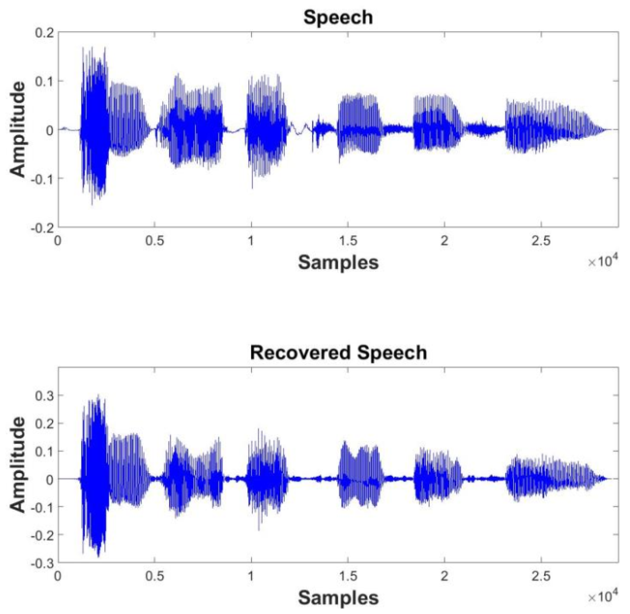
5.5. Generalization to Different Speaker

We conducted trials with different speakers to further evaluate the efficacy of the proposed technique. The training data came from one speaker, while the testing data came from another speaker. Speech was mixed with music for the training set, and the system was evaluated by using mixtures of speeches from different speaker mixed with the same music. The training dataset comprised 10 utterances from a speaker mixed with guitar music at 0 dB, whereas the testing dataset comprised another 10 utterances from a different speaker mixed with the same music at 0 dB. It is worth noting that the selected speeches by various speakers were also different. Figure 10 depicts the SDR performance. Although the proposed system was trained with different speeches, the separation performance stayed robust with little fluctuation. When music and utterances from speaker 2 were mixed, the SDR performance was 9.97 dB. The DNN, on the other hand, provided 6.85 dB. The original speech and recovered speech are displayed in Figure 11 to further demonstrate the separation performance of the proposed technique. When compared to the original speech, it can be noted that the recovered speech was quite similar to it, demonstrating the capabilities of our proposed technique.

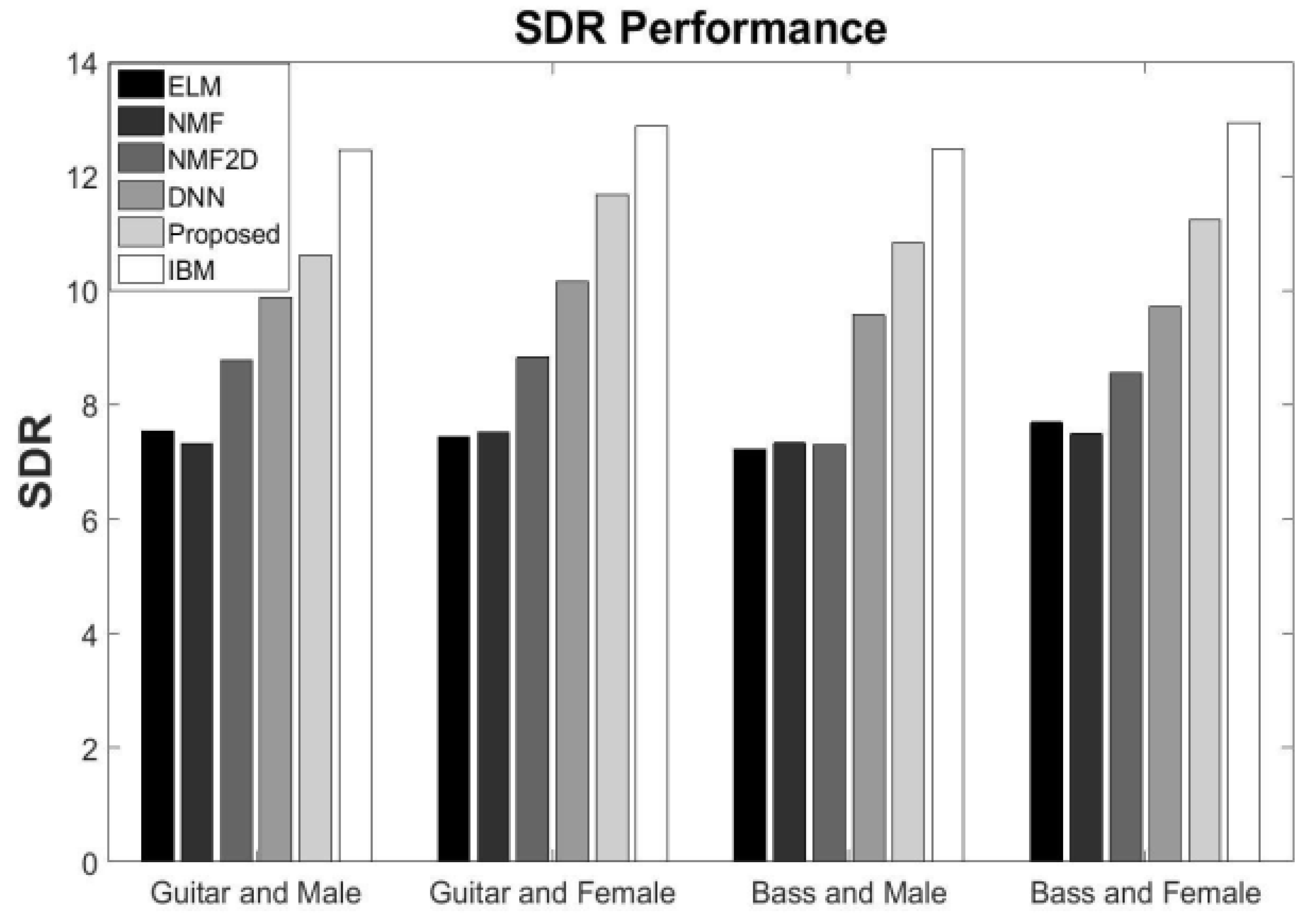
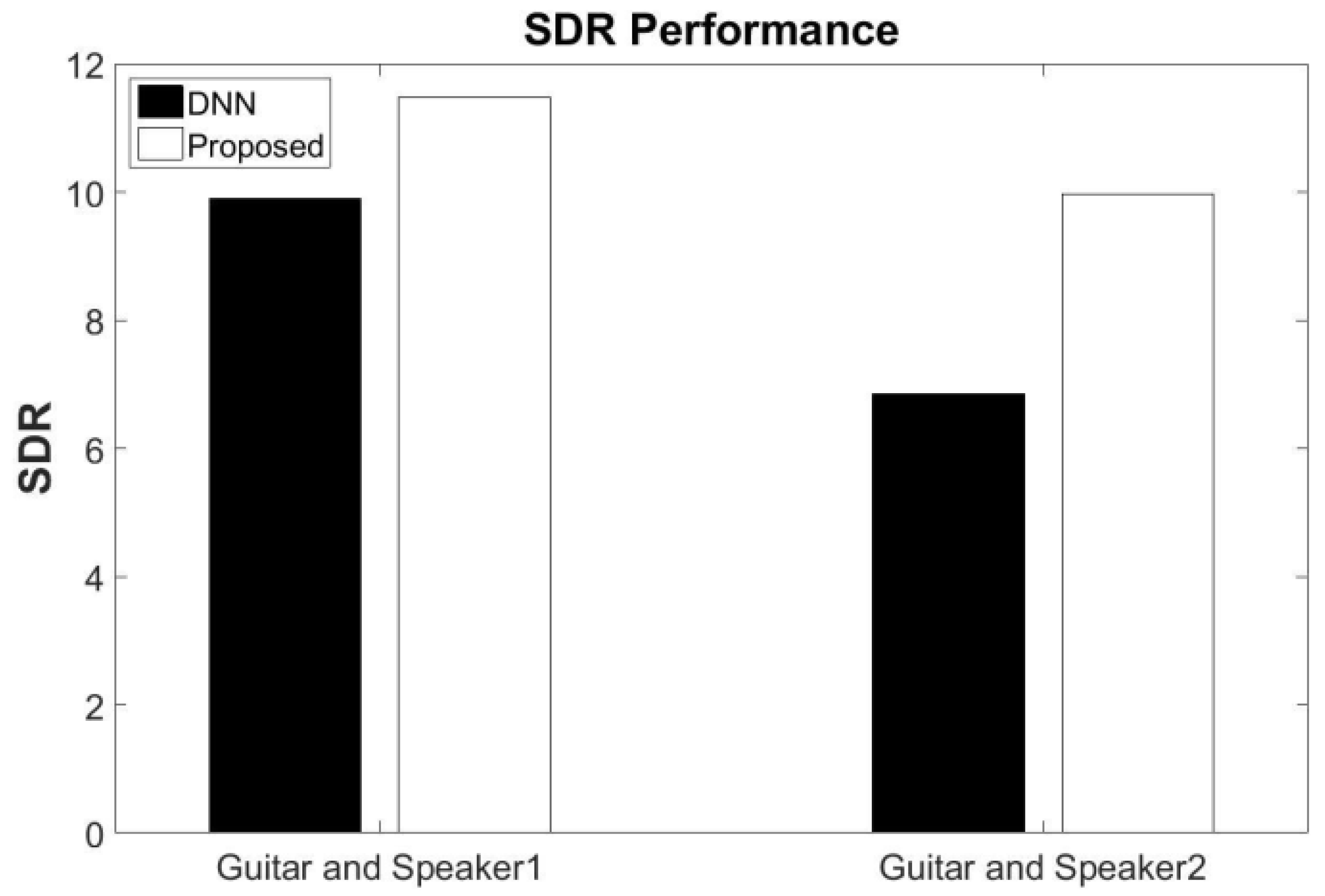
5.6. Comparisons with the Baseline Result

Table 1. The comparative result between the proposed approach and the baseline result.

	Method	Training Time (s)	Testing Accuracy (%)
Guitar and Male	MLP	3335	93.8 ± 0.4
	DNN	5667	97.4 ± 0.2
	DSELM	8.84	98.7 ± 0.3
Guitar and Female	MLP	3146	94.1 ± 0.5
	DNN	5326	97.2 ± 0.2
	DSELM	8.39	99.2 ± 0.2
Bass and Male	MLP	3261	92.5 ± 0.4
	DNN	5438	96.4 ± 0.3
	DSELM	8.21	98.3 ± 0.3
Bass and Female	MLP	3094	93.9 ± 0.4
	DNN	5296	97.1 ± 0.2
	DSELM	8.36	98.9 ± 0.2

shows the comparison of the suggested approach’s computational effectiveness and efficiency when the MLP was trained by using the back-propagation methodology and the DNN was trained by using the Restricted Boltzmann Machine (RBM) pretraining method. Since the hierarchical structure allows for the extraction of higher-order correlations between the input data, the MLP was chosen as the baseline for the deep architecture. The MLP may, however, become trapped at local minima quite readily. By using the layer-wise pretraining strategy, the DNN has made promising progress when compared to the MLP [57]. The DNN is, however, supplemented by a high computational complexity and significant time consumption. The Deep Sparse Extreme Learning Machine (DSELM) discussed before is an alternative, and its performance will be contrasted in terms of its training duration and testing precision. In order to train the deep frameworks, we chose 400 utterances from each man and female together with guitar and bass music [53], whereas 50 utterances that were not part of the training set were chosen as the testing data. The input data were standardized to a mean and unit variance of zero before being used to train the MLP and DNN. A total of 50 epochs were used for the back-propagation training of MLP. For the DNN, we employed 50 iterations of gradient descent to pretrain the RBM, which serves as the network’s fundamental building block, and 50 iterations to finetune the whole network. We utilized a learning rate of 0.001 to train the first Gaussian–Bernoulli RBM and a learning rate of 0.01 to train the previously mentioned Bernoulli–Bernoulli RBM.

The findings shown in Table 1 show how the DSELM compared to the MLP and DNN in terms of the training time and testing accuracy. The frame of the magnitude spectrogram of the speech and music was the input for these designs. It should be noted that when using the same training data, the DSELM executed far more quickly than the MLP and DNN. This is mostly attributable to the DSELM’s straightforward training process without gradual finetuning. This is in contrast to the MLP and DNN, which require repetitive backpropagation algorithm training and repeated finetuning before the network is ready for use, respectively. Additionally, before training and testing the MLP and DNN, the input data have to be normalized to a mean and unit covariance of zero. Our proposed approach, on the other hand, does not require additional data preprocessing, which is one of its advantages over the MLP and DNN. Data preprocessing may introduce bias in the estimation of the mixing gains. Referring to Table 1, it is generally noted that the DSELM not only outperformed the MLP and DNN in terms of the training time, but also in terms of the testing accuracy. For all types of mixtures, the MLP and DNN delivered average accuracies of 93.57% ± 0.4% and 97.02% ± 0.2% while the DSELM had an average accuracy of 98.78% ± 0.2%. In addition, the proposed method had a high learning speed and high accuracy and lower computational complexity, and the separation performance was improved.

In addition, Single-Channel Source Separation (SCSS) is a challenging problem in signal processing. It involves separating multiple sources that are mixed together in a single channel. One of the main challenges in SCSS is dealing with interference, which refers to the presence of other sources in the same channel that can make it difficult to separate the desired source. Reducing interference response times can be important in some SCSS research, especially in applications where real-time processing is required. For example, in speech enhancement applications, reducing the interference response times can help improve the quality of the separated speech signal by reducing the delay between the original speech signal and the processed signal.

However, for other SCSS research, reducing the interference response times may not be as important. For example, in some music-source separation applications, the goal may be to separate the sources offline without the need for real-time processing. In this case, the processing time is less important than the quality of the separated sources. In short, the importance of reducing interference response times in SCSS research depends on the specific application and the requirements of the system. Furthermore, the real-time processing of audio signals requires low latency and efficient algorithms. However, this may not be the primary concern in all applications of Single-Channel Source Separation. For example, in some offline applications such as audio restoration or audio forensics, the processing time is less critical compared to the quality of the separated sources. In this work, the interference response time was not a priority.

6. Conclusions

The motivation for this study was the fact that although the machine learning algorithms used to estimate the optimum binary mask have had considerable success at tackling single-channel audio separation difficulties, their performance level remains undesirable. An ensemble system of DNNs with stacking was proposed in this paper. By using varying initializations of each DNN in the module, the DNN ensemble system extracted various features. Furthermore, by analyzing each DNN’s complementary attribute, the system could extract the most discriminative features, which consequently improved the binary mask estimate accuracy. The activation of the penultimate layer of each DNN enabled the learning of distributed and hierarchical representations. Our experiments revealed that the proposed technique resulted in a considerably better separation performance compared with conventional methods. The proposed method had a high learning speed and high accuracy and lower computational complexity, and the separation performance was improved.

In future work, we will try to investigate areas such as informed source separation and deep reinforcement learning.

References

1. Brown, G.J.; Cooke, M. Computational auditory scene analysis. Comput. Speech Lang. 1994, 8, 297–336. [Google Scholar] [CrossRef]
2. Wang, D. On ideal binary mask as the computational goal of auditory scene analysis. In Speech Separation by Humans and Machines; Springer: New York, NY, USA, 2005; pp. 181–197. [Google Scholar]
3. Xia, T.; Tao, D.; Mei, T.; Zhang, Y. Multiview spectral embedding. IEEE Trans. Syst. Man, Cybern. Part B Cybern. 2010, 40, 1438–1446. [Google Scholar]
4. Shao, L.; Wu, D.; Li, X. Learning deep and wide: A spectral method for learning deep networks. IEEE Trans. Neural Netw. Learn. Syst. 2014, 25, 2303–2308. [Google Scholar] [CrossRef]
5. Garau, G.; Renals, S. Combining spectral representations for large-vocabulary continuous speech recognition. IEEE Trans. Audio Speech Lang. Process. 2008, 16, 508–518. [Google Scholar] [CrossRef] [Green Version]
6. Grais, E.M.; Roma, G.; Simpson, A.J.; Plumbley, M.D. Two-stage single-channel audio source separation using deep neural networks. IEEE/ACM Trans. Audio Speech Lang. Process. 2017, 25, 1773–1783. [Google Scholar] [CrossRef] [Green Version]
7. Wang, Y.; Du, J.; Dai, L.R.; Lee, C.H. A gender mixture detection approach to unsupervised single-channel speech separation based on deep neural networks. IEEE/ACM Trans. Audio Speech Lang. Process. 2017, 25, 1535–1546. [Google Scholar] [CrossRef]
8. Zhao, M.; Yao, X.; Wang, J.; Yan, Y.; Gao, X.; Fan, Y. Single-channel blind source separation of spatial aliasing signal based on stacked-LSTM. Sensors 2021, 21, 4844. [Google Scholar] [CrossRef] [PubMed]
9. Hwang, W.L.; Ho, J. Null space component analysis of one-shot single-channel source separation problem. IEEE Trans. Signal Process. 2021, 69, 2233–2251. [Google Scholar] [CrossRef]
10. Duong, T.T.H.; Duong, N.Q.; Nguyen, P.C.; Nguyen, C.Q. Gaussian modeling-based multichannel audio source separation exploiting generic source spectral model. IEEE/ACM Trans. Audio Speech Lang. Process. 2018, 27, 32–43. [Google Scholar] [CrossRef] [Green Version]
11. Pezzoli, M.; Carabias-Orti, J.J.; Cobos, M.; Antonacci, F.; Sarti, A. Ray-space-based multichannel nonnegative matrix factorization for audio source separation. IEEE Signal Process. Lett. 2021, 28, 369–373. [Google Scholar] [CrossRef]
12. Jin, Y.; Tang, C.; Liu, Q.; Wang, Y. Multi-head self-attention-based deep clustering for single-channel speech separation. IEEE Access 2020, 8, 100013–100021. [Google Scholar] [CrossRef]
13. Li, Y.; Zhang, W.T.; Lou, S.T. Generative adversarial networks for single channel separation of convolutive mixed speech signals. Neurocomputing 2021, 438, 63–71. [Google Scholar] [CrossRef]
14. Luo, Y.; Mesgarani, N. Conv-tasnet: Surpassing ideal time–frequency magnitude masking for speech separation. IEEE/ACM Trans. Audio Speech Lang. Process. 2019, 27, 1256–1266. [Google Scholar] [CrossRef] [Green Version]
15. Gu, R.; Zhang, S.X.; Xu, Y.; Chen, L.; Zou, Y.; Yu, D. Multi-modal multi-channel target speech separation. IEEE J. Sel. Top. Signal Process. 2020, 14, 530–541. [Google Scholar] [CrossRef] [Green Version]
16. Encinas, F.G.; Silva, L.A.; Mendes, A.S.; González, G.V.; Leithardt, V.R.Q.; Santana, J.F.D.P. Singular spectrum analysis for source separation in drone-based audio recording. IEEE Access 2021, 9, 43444–43457. [Google Scholar] [CrossRef]
17. Zeghidour, N.; Grangier, D. Wavesplit: End-to-end speech separation by speaker clustering. IEEE/ACM Trans. Audio Speech Lang. Process. 2021, 29, 2840–2849. [Google Scholar] [CrossRef]
18. Mika, D.; Budzik, G.; Jozwik, J. Single channel source separation with ICA-based time-frequency decomposition. Sensors 2020, 20, 2019. [Google Scholar] [CrossRef] [Green Version]
19. Jiang, D.; He, Z.; Lin, Y.; Chen, Y.; Xu, L. An improved unsupervised single-channel speech separation algorithm for processing speech sensor signals. Wirel. Commun. Mob. Comput. 2021, 2021, 6655125. [Google Scholar] [CrossRef]
20. Slizovskaia, O.; Haro, G.; Gómez, E. Conditioned source separation for musical instrument performances. IEEE/ACM Trans. Audio Speech Lang. Process. 2021, 29, 2083–2095. [Google Scholar] [CrossRef]
21. Li, L.; Kameoka, H.; Makino, S. Majorization-minimization algorithm for discriminative non-negative matrix factorization. IEEE Access 2020, 8, 227399–227408. [Google Scholar] [CrossRef]
22. Smith, S.; Pischella, M.; Terré, M. A moment-based estimation strategy for underdetermined single-sensor blind source separation. IEEE Signal Process. Lett. 2019, 26, 788–792. [Google Scholar] [CrossRef]
23. Du, J.; Tu, Y.; Dai, L.R.; Lee, C.H. A regression approach to single-channel speech separation via high-resolution deep neural networks. IEEE/ACM Trans. Audio Speech Lang. Process. 2016, 24, 1424–1437. [Google Scholar] [CrossRef]
24. Nugraha, A.A.; Liutkus, A.; Vincent, E. Multichannel audio source separation with deep neural networks. IEEE/ACM Trans. Audio Speech Lang. Process. 2016, 24, 1652–1664. [Google Scholar] [CrossRef] [Green Version]
25. Zhang, X.; Zhang, H.; Nie, S.; Gao, G.; Liu, W. A pairwise algorithm using the deep stacking network for speech separation and pitch estimation. IEEE/ACM Trans. Audio Speech Lang. Process. 2016, 24, 1066–1078. [Google Scholar] [CrossRef]
26. Wang, Y.; Wang, D. Towards scaling up classification-based speech separation. IEEE Trans. Audio Speech Lang. Process. 2013, 21, 1381–1390. [Google Scholar] [CrossRef] [Green Version]
27. Wang, Q.; Woo, W.L.; Dlay, S.S. Informed single-channel speech separation using HMM–GMM user-generated exemplar source. IEEE/ACM Trans. Audio Speech Lang. Process. 2014, 22, 2087–2100. [Google Scholar] [CrossRef]
28. Tengtrairat, N.; Gao, B.; Woo, W.L.; Dlay, S.S. Single-channel blind separation using pseudo-stereo mixture and complex 2-D histogram. IEEE Trans. Neural Netw. Learn. Syst. 2013, 24, 1722–1735. [Google Scholar] [CrossRef] [PubMed]
29. Ming, J.; Srinivasan, R.; Crookes, D.; Jafari, A. CLOSE—A data-driven approach to speech separation. IEEE Trans. Audio Speech Lang. Process. 2013, 21, 1355–1368. [Google Scholar] [CrossRef]
30. Kim, W.; Stern, R.M. Mask classification for missing-feature reconstruction for robust speech recognition in unknown background noise. Speech Commun. 2011, 53, 1–11. [Google Scholar] [CrossRef]
31. Hu, G.; Wang, D. Monaural speech segregation based on pitch tracking and amplitude modulation. IEEE Trans. Neural Netw. 2004, 15, 1135–1150. [Google Scholar] [CrossRef] [PubMed]
32. Gao, B.; Woo, W.L.; Dlay, S.S. Unsupervised single-channel separation of nonstationary signals using Gammatone filterbank and itakura–saito nonnegative matrix two-dimensional factorizations. IEEE Trans. Circuits Syst. I Regul. Pap. 2012, 60, 662–675. [Google Scholar] [CrossRef]
33. Huang, G.B.; Zhu, Q.Y.; Siew, C.K. Extreme learning machine: Theory and applications. Neurocomputing 2006, 70, 489–501. [Google Scholar] [CrossRef]
34. Yang, Y.; Wu, Q.J. Extreme learning machine with subnetwork hidden nodes for regression and classification. IEEE Trans. Cybern. 2015, 46, 2885–2898. [Google Scholar] [CrossRef] [PubMed]
35. Tang, J.; Deng, C.; Huang, G.B. Extreme learning machine for multilayer perceptron. IEEE Trans. Neural Netw. Learn. Syst. 2015, 27, 809–821. [Google Scholar] [CrossRef]
36. Huang, G.B.; Zhou, H.; Ding, X.; Zhang, R. Extreme learning machine for regression and multiclass classification. IEEE Trans. Syst. Man, Cybern. Part B Cybern. 2011, 42, 513–529. [Google Scholar] [CrossRef] [PubMed] [Green Version]
37. Kim, G.; Lu, Y.; Hu, Y.; Loizou, P.C. An algorithm that improves speech intelligibility in noise for normal-hearing listeners. J. Acoust. Soc. Am. 2009, 126, 1486–1494. [Google Scholar] [CrossRef] [PubMed] [Green Version]
38. Wang, Y.; Han, K.; Wang, D. Exploring monaural features for classification-based speech segregation. IEEE Trans. Audio Speech Lang. Process. 2012, 21, 270–279. [Google Scholar] [CrossRef] [Green Version]
39. Hermansky, H.; Morgan, N. RASTA processing of speech. IEEE Trans. Speech Audio Process. 1994, 2, 578–589. [Google Scholar] [CrossRef] [Green Version]
40. Al-Kaltakchi, M.; Woo, W.L.; Dlay, S.; Chambers, J.A. Evaluation of a speaker identification system with and without fusion using three databases in the presence of noise and handset effects. EURASIP J. Adv. Signal Process. 2017, 2017, 80. [Google Scholar] [CrossRef] [Green Version]
41. Al-Kaltakchi, M.; Al-Nima, R.R.O.; Abdullah, M.A.; Abdullah, H.N. Thorough evaluation of TIMIT database speaker identification performance under noise with and without the G. 712 type handset. Int. J. Speech Technol. 2019, 22, 851–863. [Google Scholar] [CrossRef]
42. Al-Kaltakchi, M.; Al-Nima, R.R.O.; Abdullah, M.A. Comparisons of extreme learning machine and backpropagation-based i-vectorapproach for speaker identification. Turk. J. Electr. Eng. Comput. Sci. 2020, 28, 1236–1245. [Google Scholar] [CrossRef]
43. Al-Kaltakchi, M.; Abdullah, M.A.; Woo, W.L.; Dlay, S.S. Combined i-vector and extreme learning machine approach for robust speaker identification and evaluation with SITW 2016, NIST 2008, TIMIT databases. Circuits Syst. Signal Process. 2021, 40, 4903–4923. [Google Scholar] [CrossRef]
44. Hinton, G.E. A practical guide to training restricted Boltzmann machines. In Neural Networks: Tricks of the Trade, 2nd ed.; Springer: Berlin/Heidelberg, Germany, 2012; pp. 599–619. [Google Scholar]
45. Erhan, D.; Courville, A.; Bengio, Y.; Vincent, P. Why does unsupervised pre-training help deep learning? In Proceedings of the Thirteenth International Conference on Artificial Intelligence and Statistics, JMLR Workshop and Conference Proceedings, Sardinia, Italy, 13–15 May 2010; pp. 201–208. [Google Scholar]
46. Mohammad, A.S.; Nguyen, D.H.H.; Rattani, A.; Puttagunta, R.S.; Li, Z.; Derakhshani, R.R. Authentication Verification Using Soft Biometric Traits. U.S. Patent 10,922,399, 16 February 2021. [Google Scholar]
47. Mohammad, A.S. Multi-Modal Ocular Recognition in Presence of Occlusion in Mobile Devices; University of Missouri-Kansas City: Kansas City, MO, USA, 2018. [Google Scholar]
48. Mohammad, A.S.; Rattani, A.; Derakhshani, R. Comparison of squeezed convolutional neural network models for eyeglasses detection in mobile environment. J. Comput. Sci. Coll. 2018, 33, 136–144. [Google Scholar]
49. Mohammad, A.S.; Reddy, N.; James, F.; Beard, C. Demodulation of faded wireless signals using deep convolutional neural networks. In Proceedings of the 2018 IEEE 8th Annual Computing and Communication Workshop and Conference (CCWC), Las Vegas, NV, USA, 8–10 January 2018; pp. 969–975. [Google Scholar]
50. Bezdek, J.; Hathaway, R. Some notes on alternating optimization. In Advances in Soft Computing—AFSS 2002; Springer: Berlin/Heidelberg, Germany, 2002; pp. 187–195. [Google Scholar]
51. Bhatia, R. Matrix Analysis; Springer Science & Business Media: Berlin/Heidelberg, Germany, 2013; Volume 169. [Google Scholar]
52. Barker, J.; Vincent, E.; Ma, N.; Christensen, H.; Green, P. The PASCAL CHiME speech separation and recognition challenge. Comput. Speech Lang. 2013, 27, 621–633. [Google Scholar] [CrossRef] [Green Version]
53. Goto, M.; Hashiguchi, H.; Nishimura, T.; Oka, R. RWC Music Database: Music Genre Database and Musical Instrument Sound Database. 2003. Available online: http://jhir.library.jhu.edu/handle/1774.2/36 (accessed on 23 April 2023).
54. Ellis, D. PLP, RASTA, and MFCC, Inversion in Matlab. 2005. Available online: http://www.ee.columbia.edu/~dpwe/resources/matlab/rastamat/ (accessed on 23 April 2023).
55. Févotte, C.; Bertin, N.; Durrieu, J.L. Nonnegative matrix factorization with the Itakura-Saito divergence: With application to music analysis. Neural Comput. 2009, 21, 793–830. [Google Scholar] [CrossRef]
56. Taal, C.H.; Hendriks, R.C.; Heusdens, R.; Jensen, J. An algorithm for intelligibility prediction of time–frequency weighted noisy speech. IEEE Trans. Audio Speech Lang. Process. 2011, 19, 2125–2136. [Google Scholar] [CrossRef]
57. Bengio, Y. Learning deep architectures for AI. Found. Trends Mach. Learn. 2009, 2, 1–127. [Google Scholar] [CrossRef]
Figure 1. The architecture of the proposed work.
Information 14 00352 g001
Figure 2. The performance of Short-Time Objective Intelligibility (STOI).
Information 14 00352 g002
Figure 3. The performance of Perceptual Evaluation of Speech Quality (PESQ) (a) and Signal-to-Distortion Ratio (SDR) (b).
Information 14 00352 g003
Figure 4. Signal-to-Distortion Ratio (SDR) performance for different mixture.
Information 14 00352 g004
Figure 5. Time domain separation results. (a) Mixture of guitar and female utterance. (b) Female utterance. (c) Recovered speech. (d) Music. (e) Recovered music.
Information 14 00352 g005
Figure 6. Short-Time Objective Intelligibility (STOI) under different SNRs.
Information 14 00352 g006
Figure 7. Signal-to-Distortion Ratio (SDR) performance under different SNRs.
Information 14 00352 g007
Figure 8. Signal-to-Distortion Ratio (SDR) with unmatched Bass and Piano music.
Information 14 00352 g008
Figure 9. Separation performance based on different input music.
Information 14 00352 g009
Figure 10. Signal-to-Distortion Ratio (SDR) with unmatched Guitar music.
Information 14 00352 g010
Figure 11. Original speech and recovered speech.
Information 14 00352 g011