Article

Using Genetic Algorithms to Improve Airport Pavement Structural Condition Assessment: Code Development and Case Study

1
Department of Economics, University of Messina, 98122 Messina, Italy
2
Department of Mathematics, University of California Riverside, Riverside, CA 92521, USA
3
Department MIFT, University of Messina, 98158 Messina, Italy
*
Author to whom correspondence should be addressed.
Information 2023, 14(5), 286; https://doi.org/10.3390/info14050286
Submission received: 28 February 2023 / Revised: 6 May 2023 / Accepted: 9 May 2023 / Published: 11 May 2023
(This article belongs to the Special Issue Machine Intelligence in Interdisciplinary Areas)

Abstract

:
In this paper, we propose a new method of optimization based on genetic algorithms using the MATLAB toolbox “Global Optimization”. The algorithm finds layers moduli of a flexible pavement through the measurement of pavement surface deflections under assigned load conditions. First, the algorithm for the forward calculation is validated, then the algorithm for the back-calculation is proposed, and the results are compared, in the case of airport pavements, with other software using different back-calculation techniques. The goodness of the procedure and the way of managing the algorithm operator is demonstrated by means of positive feedback obtained from the comparison of the results of ELMOD and BackGenetic3D. Moreover, the findings of the analysis prove that, in such an optimization procedure by GA, the best solution is always reached with a low number of generations, generally less than 10, allowing a reduction in the time of calculation and choosing a population big enough to select with good probability, in the initial population, solutions close to the real ones. The code is made available in such a way that the reader can easily apply it to other flexible pavements in the case of fully bonded layers (both for roads and airports). In particular, interested readers can easily modify the algorithm parameters (population number, stop criteria, probability of mutation, cross-over, and reproduction) and the type of fitness function to minimize, together with the geometric and load characteristics (number and thickness of the layers and the range of module variation). The possibility to change the algorithm parameters and the fitness function allows for exploring different scenarios in order to find the best solution in terms of fitness values. It is also possible to intervene in the time of calculation by managing the algorithm’s stopping criteria.

1. Introduction

The process of evaluating the layer moduli of a pavement using the deflection data is defined as back-calculation (backward calculation). This technique specifically selects the modules of the layers using any suitable methodology (iteration, database search, closed-form solutions, or optimization) that produces deflections as close as possible to those measured by the instrument [1].
Back-calculation is a procedure that allows deriving instantaneous information of the mechanical characteristics of the layers of a pavement—through the measurement of the pavement’s surface deflection under certain load conditions [2]. The above analysis is essential to evaluating pavement service conditions, predicting its performance and residual life, and evaluating the type and time of intervention needed to remedy any structural deficiencies.
Back-calculation of pavement layer moduli has been a topic studied for more than five decades [3,4]. Indeed, the evaluation of appropriate mechanical characteristics for the various layers is key to the design of new and in-service pavements and, in particular, is useful for:
  • Assessing the conditions of service of the pavement,
  • Predicting the performance and residual life of the pavement,
  • Formulating maintenance and rehabilitation strategies,
  • Selecting the types of treatment to be performed,
  • Carrying out, if requested, the design of an additional layer.
Despite the existence of many back-calculation programs, which use different algorithms and procedures, the accuracy of the moduli values is still controversial. The procedures that require the initial moduli to start the back-calculation process generally find different solutions for different initial moduli, which can lead to very different pavement evaluations. Indeed, in the search space exists many local optima, and so more than one solution could satisfy the criterion of the objective function.
Moreover, it is also recommended to use a maximum of three layers to reduce the errors associated with the back-calculation process.
Genetic Algorithms (GAs), which operate using guided random search techniques, can be used for the back-calculation of pavement modules since they are able to consider the entire global search space of the objective function, overcoming the problem of local maxima [5]. GAs are based on Darwinian theory and are formulated on the mechanics of genetics and natural selection [6,7].
The objective of this work is to show how it is possible to optimize the procedure of back-calculation of pavement layer moduli through the use of genetic algorithms. The procedure allows for evaluating the mechanical properties of a pavement, which is essential for forecasting a declining law and intervention time for pavement maintenance.

2. Background

2.1. Pavement Response of Elastic Multi-Layer System

Scrivner et al. [8] developed the first closed-form solution that finds the pavement response of a two-layer system based on the Burmister layer theory [9]. The first solution in closed form for evaluating the layer modules of a multi-layer pavement was developed by Yih Hou [10] using the least squares method. The first graphic method to determine the modules of a two-layer system was developed by Swift [11]. In some back-calculation models, the Odemark equivalent layer concept [12] has been used to simplify the multi-layer systems, allowing the use of the Boussinesq theory [13]. The back-calculation method developed by Ullidtz [14] is based on this concept and gives reasonable moduli values for pavements in which the stiffness of the layers decreases with depth. Lytton and Michalak [15] used a more general form of the Odemark hypothesis to convert a multi-layer system into a single layer lying on a rigid base. With the advances that have taken place from a computational point of view, a series of computer back-calculation programs are available.
Back-calculation procedures are generally associated with a suitable response theory of stratified systems, with an optimization technique for the selection of a set of layer modules that produce calculated responses similar to the measured responses to an objective function that reflects the differences between measured and calculated deflections.
Generally, all commonly used back-calculation methods assume flexible pavements are linear elastic multi-layer systems and employ an iterative approach that starts with some test modules to find a set of modules, for the various layers, that produce, under a load application, a deflections basin as close as possible to the measured deflections basin.
When the FWD is used, the measured deflection basin is represented by the measurements detected by the sensors. The deflections basin calculated is generally obtained using the elastic multi-layer theory, assuming a static load. The objective function, therefore, has the aim of minimizing errors (within a specified tolerance value), which are the differences between calculated and measured deflections.
To guard against unforeseen circumstances or incorrect inputs, generally, all back-calculation programs include setting a maximum number of iterations as one of the stopping criteria. The results vary according to the response model of the system and the calculation software used, the method by which the modules are generated, the method of searching for modules by the algorithm, the objective function, and the sensitivity of the algorithm with respect to errors in deflection measurements and layer thicknesses, etc.
The classical methods of moduli back-calculation have several limitations, also theoretical limitations, that do not allow us to find the “real” moduli. In classical methods, the thickness and elastic modulus of pavement with several layers are considered equivalent to the first layer. Therefore, it is always necessary to modify them with correction factors that depend on the pavement system. The regression equation-based approach [16,17] or the back-calculation method by search on database [18,19] have the defect of only being valid for the specific pavement and for the load conditions for which they were derived. Another problem is the non-uniqueness of the solution, which cannot be effectively managed by one of these methods. This problem is further aggravated by the inevitable presence of errors in the deflection measurements.
Moreover, a major limitation of almost every back-calculation procedure is the consideration of linear elastic materials for all pavement layers. Indeed, the asphalt layers in the flexible pavements show both elastic and viscous features. At high temperatures, the viscoelastic behavior dominates, and the pavement damage for airport pavements can be even double (e.g., [20,21]), with a profound impact on the decision-making processes. At low temperatures, linear–elastic models could be sufficient to model the material parameters [22]. Accordingly, when using deflections to assess the structural performance of pavement, deflections should be corrected for temperature and adjusted to the same reference temperature [23] in order to better reflect the pavement’s structural strength.

2.2. Back-Calculation through the Use of a GA

In the last years, in several managerial fields, there has been a drastic increase in the use of deep learning and soft computing for the resolution of optimization problems with one or more objective functions that difficultly could be solved in a closed way. For instance, the minimization of the production costs or of the environmental impact of products or processes, accordingly to a life-cycle assessment analysis [24] or the search for Nash equilibrium in a multi-player decision game theory model [25]. In engineering applications, the cost optimization of road pavement thickness design [26] or the optimization in pavement rehabilitation and maintenance decisions [27]. All these problems are solved by using GA.
In the back-calculation of pavement layer moduli, specifically, GAs are revealed to be very useful, thanks to their capacity to examine the global search space of possible solutions and to overcome the problem of local maxima [5]. For this reason, many authors have used genetic algorithms for the optimization of that problem [3,28], studying possible efficient parameters of the GA [29,30], and also proposing software that conducts the back-calculation process in particular conditions [31]. All recent methods continue using GA, for instance, together with Multi-Layer Elastic Theory (MLET) for investigating the performance of the foamed asphalt base [32]. New hybridized methods use GAs for the optimization of moduli back-calculation together with artificial neural networks (ANN) for the prediction of pavement deflection basin [33,34]. For instance, ANN–GA methods are developed considering the viscoelastic properties of the asphalt layer and nonlinear parameters of unbound layers [35,36,37]. This procedure with ANN requires the phase of training and verification using a synthetic database.
In the analysis proposed in this article, we used MLET for determining deflection and GAs for optimization because, as previously said, GAs present an interesting approach to overcoming the local maxima problem thanks to the ability to “move out” from the local maximum and to explore new regions of the decision-making space where there is high probability of finding solutions with a better fitness value. A GA does not require the initial moduli, and the method of back-calculation using a GA is suitable for parallel computers and operations with a large number of parameters.
Therefore, we propose a new method of optimization by a GA using the MATLAB toolbox “Global Optimization”. The code is made available in Appendix A in such a way that the reader can easily apply it to other flexible pavements in case of fully bonded layers (both for roads and airports). In particular, the interested readers can easily modify the algorithm parameters (population number, stop criteria, probability of mutation, cross-over, reproduction) and the type of fitness function to minimize, together with the geometric and load characteristics (number and thickness of the layers, the range of module variation). The possibility to change the algorithm parameters and the fitness function allows us to explore different scenarios in order to find the best solution in terms of fitness values. It is also possible to intervene in the time of calculation by managing the algorithm-stopping criteria.

3. Method: Back-Calculation with GA

The first step in the back-calculation procedure is the determination of an algorithm for the forward calculation, that is, the evaluation of the pavement response model. Then, it is necessary to define the fitness function to satisfy.
The response model of the pavement should provide the deflection of any point of the pavement as the distance from the loading axis varies, following the application of a load distributed over a certain area of radius a.
Usually, for flexible pavement, a 3-layer system is used: bitumen-bonded layer, foundation in granular- or cement-stabilized mixture, and substrate. For a flexible three-layer pavement, the theory of elastic multi-layer [38] is simplified in the following Equations (1)–(3).
In the below formulas, all the quantities are normalized with respect to the distance H between the surface of the pavement and the surface of the n-th layer.
The quantities are defined as following:
  • α = a/H, where a is the radius of the footprint of the uniformly distributed circular load [m];
  • λ = z/H where z represents the depth, which starts from zero on the surface and grows downwards [m];
  • ρ = r/H where r is the distance from the axis of application of the load [m];
  • Φ = F/H where F is the force applied to the circular plate [kN].
Therefore, the pressure, defined as q = F A , is given by:
q = Φ π α 2 = F H π ( a H ) 2 = F H π a 2
The displacement w of a generic point, when the system is subjected to a load q uniformly distributed over a circular area of radius a, is a function of the normalized distance ρ with respect to the load axis and of the normalized depth λ, and it is found as:
w = q α 0 w * m   J 1 ( m   α ) d m
where:
  • J 1 is the Bessel function of the first kind and of order 1,
  • m is a parameter that takes positive values. The integral that appears in the previous relation in dm has as integration extremes 0 and the largest positive value of m, which provides a finite displacement w,
  • w * is the displacement of a generic point when the system is subjected to a vertical load of m J 0 ( m ρ ) , defined by the following expression:
( w * ) i = 1   +   ν i E i J 0 ( m   ρ ) { [ A i C i ( 2 4 ν i m λ ) ] e m ( λ i λ ) [ B i + D i ( 2 4 ν i + m λ ) ] e m ( λ λ i 1 ) }
where
-
J 0 is the Bessel function of the first type and of order 0
-
ν i is the Poisson’s ratio of the generic layer i
-
E i   is the elastic modulus of the generic layer [kPa]
-
A i ,   B i ,   C i ,   D i are the integration constants of the generic layer, which are obtained by imposing the boundary and continuity conditions
-
i varies from 1 to the number of layers and represents the considered layer
-
λ i   represents the normalized depth at the interface between layer i and i + 1
-
m has been previously defined
-
ρ and λ are variables ranging between 0 and .
The most used fitness functions to minimize in back-calculation of pavement layer moduli are:
  • The sum of the absolute differences of the deflections:
    i = 1 N w i ( D i d i )
  • The sum of the squared differences of the deflections:
    i = 1 N w i ( D i d i ) 2
  • The sum of the square of the relative errors of the deflections:
    i = 1 N w i ( D i d i D i ) 2
  • The maximum percentage error of the deflections:
      m a x ( D i d i D i ) × 100 % ,               i = 1 , 2 , , N
  • The maximum percentage error of the modulus of the layers computed in successive iterations:
  m a x ( E j ( k ) E j ( k 1 ) E j ) × 100 % ,               j = 1 , 2 , , m
where w i is the weight of sensor i; Di and di are, respectively, the deflections measured and calculated in sensor i; N is the total number of sensors that are available for deflection measurement, E j ( k ) the elastic modulus of layer j calculated in the k-th iteration and m the total number of pavement layers. It should be remembered that all N sensors are often given the same weight.
The steps of the proposed genetic algorithm procedure are the following.
  • There are assigned ranges of variation for the modules of the layers that have to be determined according to the type of material constituting them.
  • The algorithm creates an initial population formed by a certain number of individuals (number of population). Each individual represents a possible solution to the problem; therefore, each individual is associated with a set of n modules where n is the number of pavement layers. The module values are randomly selected within the variation ranges previously assigned.
  • Knowing the thicknesses and the Poisson coefficients of the pavement layers, the distances of the sensors with respect to the load axis, and the applied force, formula (3) is used to calculate the displacements of the pavement at the sensors.
  • The fitness value of each individual in the population is then determined as the difference between the displacements just calculated and those measured by the instrumentation.
  • If the fitness value of one of the individuals in the population is lower than a certain tolerance (previously fixed), the algorithm stops and returns the corresponding modules; otherwise, it passes to the next generation.
  • A new generation of individuals is created by selecting individuals who are candidates for reproduction (parents) according to their fitness value by manipulating the genes of these individuals using genetic transformation operators (reproduction, cross-over, and mutation) in order to obtain new configurations of chromosomes (children) and by inserting new individuals (based on the fitness value) in the population and replacing older individuals.
  • The fitness of the individuals of the new generation is then evaluated, and if one of these fitness values reaches the tolerance or if another stop criterion is reached, the algorithm stops and returns the values of the module; otherwise, it continues with a new generation and so on.

4. Software Validation

4.1. Implementation of the Pavement Response Model on MATLAB and Comparison of the Results with the Software KENPAVE: Direct Check

As the first step, the algorithm for the forward calculation—describing the response model of the system—was implemented on MATLAB, and subsequently, the resulting deflections were compared with the deflections, under the same conditions, obtained by another software that uses the elastic multi-layer model, which is KENPAVE.
The choice to use MATLAB is due to the presence of the associated toolbox of global optimization by GA, which is subsequently used for the back-calculation of pavement layers moduli.
The written code allows obtaining the deflection of any point (at any depth from the surface and at any radial distance from the axis) when a load of any intensity that is uniformly distributed over any area acts on a system with any number of layers defined by any sensors geometry and mechanical characteristics.
To validate the goodness of the model, the results in terms of deflections of a three-layer system with the following characteristics of geometry (layers thickness), mechanical characteristics (E modulus and Poisson coefficient), load intensity (force and radius), and position of the sensors (see Table 1) are compared.
In KENPAVE software, the deflections are evaluated at the surface (for z = 0) of a three-layer system with constrained interfaces, in the hypothesis of a linear elastic material, without a damage analysis, and considering only one period of the year and only one load group (load applied on a circular area, representing the FWD test plate).
The input is the thickness of the layers, the relative Poisson’s coefficients, and the elastic moduli. The load is a uniformly distributed pressure of 550 kPa, which corresponds to a force of 38.87 kN on a circular area of a radius of 15 cm. Six radial distances are considered with respect to the load axis to calculate the pavement response and represent the positions of the various sensors of the FWD equipment.
The results of the analysis are shown below and lead to an error of a thousandth of a millimeter, as can be seen from the comparison shown in Table 2.

4.2. Compare the Pavement Layer Moduli Obtained by a GA with the Modulus That in KENPAVE Generate the Deflections Used as Input in the Back-Calculation Procedure: Indirect Check

By putting as input data in the proposed program the displacements obtained in KENPAVE, the modules obtained by back-calculation with a GA approach actually produce those displacements in KENPAVE. For rapidity of calculation, a two-layer pavement with the following characteristics is considered (Table 3).
The deflections obtained in KENPAVE, in correspondence to the sensors placed at r1, r2, r3, r4, r5, and r6, are, respectively, 0.5565, 0.4478, 0.3871, 0.25, 0.1682, and 0.1497 mm.
They are used as input data (measured deflections) to find modules E1 and E2, which should coincide with the initial ones. Table 4 shows the results of the back-calculation for some analyses that differ in population number, number of considered sensors, breadth of moduli ranges, etc. It always starts from wide ranges, and it tries to refine the results by working with the other parameters of the algorithm so as to reach increasingly smaller values of the fitness function (i.e., a small difference between measured and calculated deflections). The analysis with the smallest fitness value gives the results of E1 = 2010.58 and E2 = 99.88, which are very similar to the real values of 2000 and 100.

5. Case Study: Application of the Optimization GA Code to a Real Case

The forward calculation of the developed system can be applied both to road and airport flexible pavements. For the numerical application, we consider an airport pavement, thus carrying out the deflection measurements using the HWD (Heavy Weight Deflectometer) equipment, which is able to apply a force that can reach up to 250 kN (representing the load produced by a fully loaded Boeing 747 wheel).
The deflection measurements were carried out in an airport with the following geometric and mechanic characteristics of the layers, load characteristics, distance of the sensors, and with the following measured deflections (data have been extracted by the Engineering Department of the University of Messina) (see Table 5).
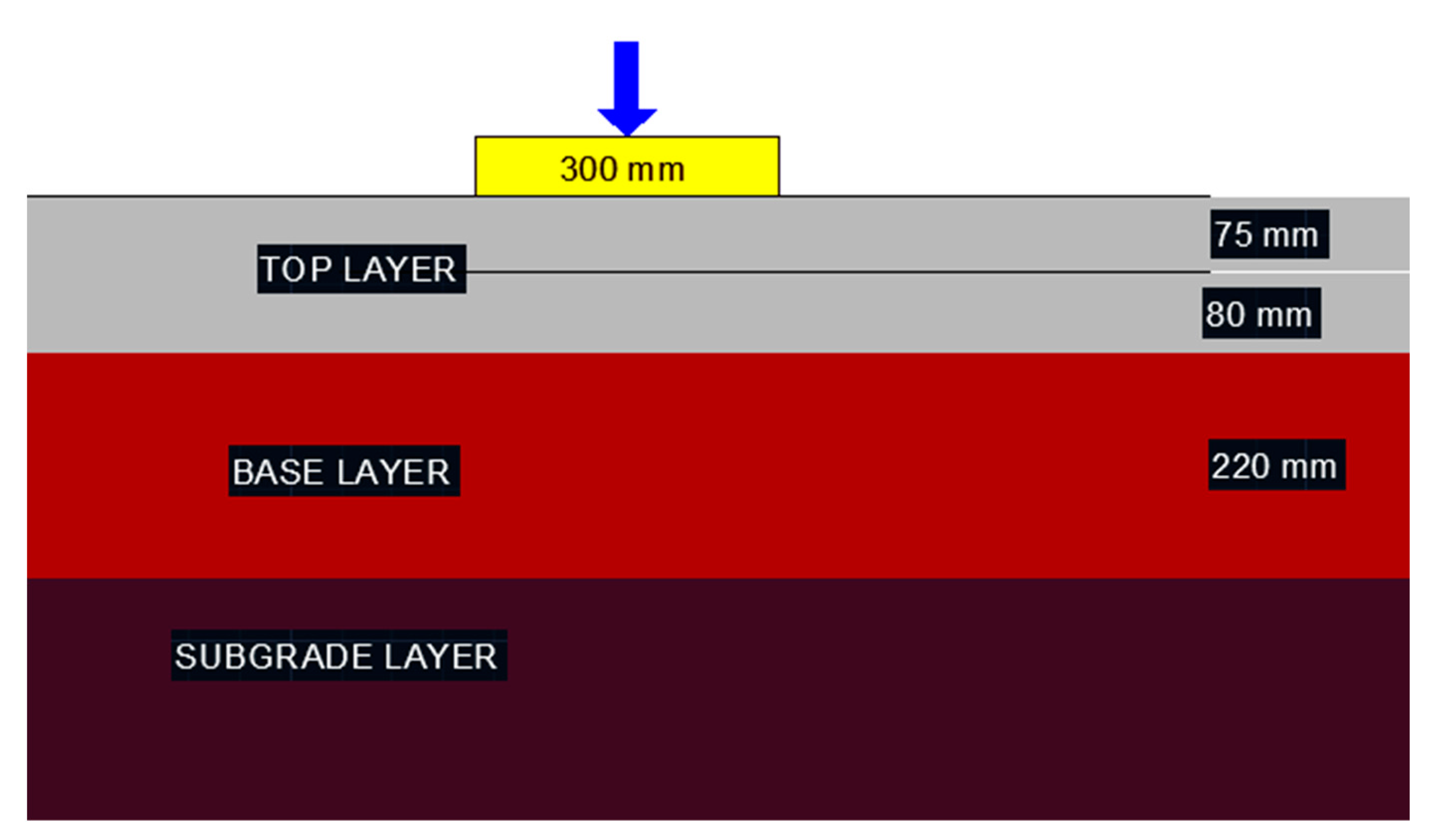
Flexible pavement is normally modeled as a three-layer system with all AC layers considered as a unified course according to common engineering sense during back-analysis (the two sub-layers—from Figure 1—correspond to surface and binder course), the base layer (in mixed granular or cement stabilized) as the second layer and the subgrade (considered as the pavement foundation layer) as the third layer.
Therefore, Figure 1 shows the first layer of AC with a thickness of 15.5 cm, a second layer of 22 cm, which represents the base, and the third and last layer in the granular mix representing the subgrade, which is assumed in the model as a layer of infinite thickness.

6. Results

In Table 6, the results of different analyses are shown, obtained by changing the parameters of the algorithms and the range of the layers moduli. The fitness function optimization problem here applied is:
M i n i m i z e i = 1 N ( d i D i ) 2 ,
That is, the minimization of the sum of the square of the differences between calculated and measured deflections, where Di and di are, respectively, the deflections measured and calculated in sensor i, and N is the total number of sensors that are available for deflection measurement.
Table 6. Back-calculation results.
(1)(2)(3)(4)(5)
Population (P)403020530
Range of modulusE1 (MPa)2000–80004500–65005000–60005000–58005000–6000
E2 (Mpa)100–20002000–40002500–38002500–38002500–3800
E3 (Mpa)50–200150–350200–300200–300200–300
Probability of cross-over0.80.80.740.80.8
Probability of mutation0.20.20.10.20.2
Calculated modulus E1 (Mpa)7480.2255589.4325278.4995078.0325850.679
E2 (Mpa)1865.6013040.1053485.0622500.0013615.922
E3 (Mpa)187.001225.479218.686248.538208.747
Fitness value 2.643 × 10−86.195 × 10−103.06 × 10−103.53 × 10−92.34 × 10−10
The first step in the solution search is to consider very large ranges of variation of the modules, especially for the bituminous conglomerate layer (where the module values vary with the temperature). Since it is not known whether the foundation is in a granular mixture or cement-stabilized, we assigned a wide enough range that could include the presence of different types of material. It can be immediately noticed that the values given by the back-calculation (see analysis (1)) are very close to the extremes of the assigned ranges, which, therefore, must be modified. In the second and third analyses, there are modules that lead to the best fitness value (i.e., the differences between deflections measured by the HWD and calculated are smaller) and which fall well within the assigned ranges. At this point, to further minimize the fitness value, the variation ranges can be tightened, and the deflections in several distance points can be compared.
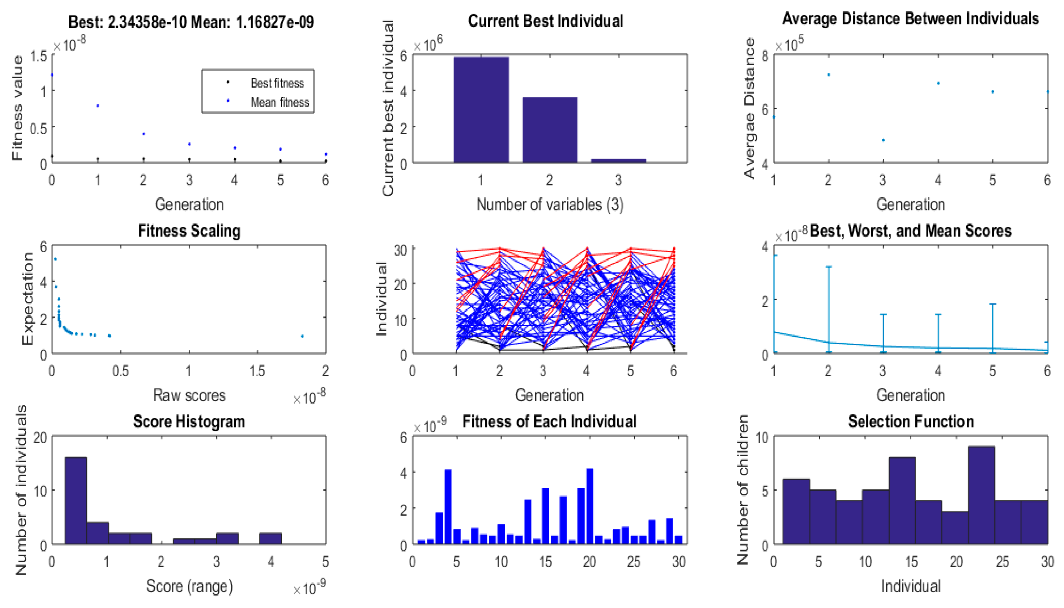
The algorithm stopping criteria set (that stop for reaching a fitness value lower than a fixed tolerance, for reaching a predetermined number of generations, or for not increasing the best fitness value after a certain number of generations) have allowed the performing of a low number of generations (6 generations in the last analysis (5) with the best fitness value), which is a big advantage considering the long computation times.
In the fourth analysis, all the measured deflections (eight sensors) are considered. The algorithm finds the optimal solution among those within the population, but then despite the use of cross-over, mutation, and other operators, it cannot greatly improve its fitness value as the generations increase. The population is too small, and the solutions are really near the range limits. It follows that population size has turned out to be one of the most important parameters. Its optimal value is the largest possible. At the same time, the calculation time is directly proportional to the size of the population, together with the number of generations and the number of considered sensors. It was, therefore, necessary to opt for a value that satisfied both needs, in any case not less than 20.
In the last analysis, a population of 30 is considered, and the optimization procedure is stopped at the sixth generation to reach one of the stopping criteria of the algorithm (the average change in the fitness value is less than the tolerance of the fitness value). The obtained moduli are E1 = 5,850,679 MPa, E2 = 3,615,922 MPa, and E3 = 208,747 MPa, which give the deflections of 0.4853 mm, 0.402 mm, 0.3666 mm, 0.3262 mm, 0.2309 mm, 0.1841 mm, 0.1487 mm, 0.1222 mm at the eight considered sensors. These deflections are very close to the deflections measured by the sensors (see Table 5).
It is found that, in such a type of optimization procedure by GA, the solution is always reached with a low number of generations, generally less than 10 (see, for instance, the first graph in Figure 2). That circumstance reduces the time of calculation and allows one to choose a population number big enough to select with good probability, in the initial population, solutions close to the real ones.
In fact, as it is easy to understand and fix the number of layers, the calculation time is given by the product between the time to evaluate the displacement of the pavement in correspondence to one sensor and the number of sensors, populations, and generations.
Figure 2 shows the plots of analysis (5) with some characteristics of the algorithm as the generation number increases.
For a check of the goodness of the results, the results of the proposed algorithm are compared with those of two other software, which are BackGenetic3D (designed by the group of Computer Modeling and Simulation at the University of Akron, combining the Multismart3D software, used for forward computation—i.e., the computation of surface deflections known the modules of the layers, —with the GA as an optimization technique in the search for the modules of the layers) and ELMOD (“Evaluation of Layer Moduli and Overlay Design” from Dynatest, uses the theory of Odemark–Boussinesqe transformed section for forward analysis, with an iterative method for back-calculation). Table 7 shows the final values of layer moduli for the examined pavement (in a specified section of the center line) and the differences in errors.
Specifically, the obtained moduli are very similar to BackGenetic3D and more distant from ELMOD. A justification is due to the use of a GA for the optimization in BackGenetic3D instead of another iterative method for back-calculation [39] used in ELMOD.
For what concerns the time of calculation, the proposed software is slower than BackGenetic3D because it uses for the forward analysis of the MLET that requires, for a pavement with three layers, the inversion of three matrices 4 × 4 for the evaluation of a single displacement. BackGenetic3D, instead, uses the Multismart3D software for forward analysis, which requires only solving two systems of linear algebraic equations (2 × 2 and 4 × 4) in the transformed domain, no matter how many layers there are in the layered structure.

7. Discussion

The proposed procedure allows the evaluation of the elastic layer moduli of a flexible pavement, knowing the surface deflection measurements under assigned load conditions. This procedure leads to the optimization of the back-calculation process thanks to the possibility of varying the GA parameters (population size, probability of genetic operators, range of variation of the variables, fitness function) and managing the error (operating on the tolerance).
That is important because the development of an algorithm that manages to find optimal results requires the use of appropriate operators and correct population size. Indeed, the selection of the GA parameters has not been generalized in the form of rules or guidelines, and none of the previous studies have been able to demonstrate that the suggested parameters are the optimal parameters that can be used for any problem [40,41].
It has to be underlined that the pavement response model implemented in MATLAB according to the MLET (see Appendix A) allows calculating the deflection of any point (at any depth from the surface and at any radial distance from the axis) when a load of any intensity that is uniformly distributed over any area acts on a system with any number and mechanical characteristics of layers defined by any sensors configuration.
Despite the advantages of using GA, it must be considered that the GA increases the computation time of the calculations, and, accordingly, only a limited number of layers and a limited number of points of the deflection basin are generally considered. The processing times of the calculations are very long because:
  • For each iteration, a number of possible solutions equal to the size of the population are evaluated.
  • For each set of modules, which represents a possible solution, a fitness value is evaluated, which indicates the goodness of the solution.
  • The fitness value of each solution requires the evaluation of a number of surface deflections equal to the number of HWD sensors.
  • The calculation of each deflection requires the inversion of three matrices 4 × 4.
Therefore, as it is easy to understand, fixed the number of layers, the calculation time is given by the product of the time to evaluate the displacement of the pavement in correspondence to one sensor by the number of the sensors, by the number of populations, by the number of generations. However, it is found here that, in such a type of optimization procedure by GA, the solution is always reached with a low number of generations, generally less than 10 (see, for instance, the first graph in Figure 2). That circumstances reduce the time of calculation and allow one to choose a population number big enough to select with good probability in the initial population provides solutions close to the real ones.
The numerical application has been addressed for a three-layer system, but the written program is easily editable for systems with any number of layers. With the use of more powerful computers in parallel, moreover, the problem of the time of calculation can be reduced.
Recently, to overcome the computational time problem, efforts have been made in the literature. For instance, a new hybridized method that uses ANN, together with the Jaya procedure for moduli optimization, has been applied to reduce the calculation time [42]. Further, a new approach with an ANN model was developed to predict pavement response directly from surface deflections without back-calculation [43], and a hybrid neural network structure, combined with a Residual Neural Network, Recurrent Neural Network, and Wide and Deep structure, was proposed [44].

8. Conclusions

This paper carefully studied the back-calculation of layers moduli of a flexible pavement by using GA. A new back-calculation algorithm is developed and implemented in MATLAB software using the Global Optimization Toolbox: genetic algorithms. That original algorithm is able to derive the layers moduli of a flexible pavement with any number of layers and any load configuration.
The algorithm for the forward calculation has been validated, and the procedure of back-calculation has been applied to a system of three layers—layers are assumed linear, homogeneous, and elastic.
The effects on the performance of the back-calculation process, population size, genetic operator probability, sensor number, and the search space range (range of module variation) have been investigated.
We have demonstrated the validity of the proposed model and of the way of managing the algorithm operators by means of the positive feedback obtained from the comparison with the results of other software such as ELMOD, developed by Dynatest, and BackGenetic3D, developed by the University of Akron, that use different back-calculation techniques.
The evaluation of the modules of the layers of an existing airport pavement is of fundamental importance since it allows to:
  • Evaluate the service conditions of the pavement,
  • Predict the performance and residual life of the pavement,
  • Evaluate the extent and type of intervention necessary to remedy any structural deficiencies,
  • Determine the maximum permissible loads.
The developed back-calculation algorithm allows modifying the algorithm parameters (population number, stop criteria, probability of mutation, cross-over, reproduction) and the type of fitness function to minimize, together with the geometric and load characteristics (number and thickness of the layers, the range of module variation). Moreover, a possible way to manage the parameters of genetic algorithms has been discussed.

Author Contributions

Conceptualization, A.D. and D.C.; methodology, A.D. and D.C.; software, A.D.; validation, A.D.; formal analysis, A.D.; data curation, A.D.; writing—original draft preparation, A.D. and D.C.; supervision, A.D. All authors have read and agreed to the published version of the manuscript.

Funding

This research received no external funding.

Data Availability Statement

Not applicable.

Conflicts of Interest

The authors declare no conflict of interest.

Appendix A

function [f] = eight(E1)
r = [ 0   0.2   0.3   0.45   0.9   1.2   1.5   1.8 ]
h 1 = 0.155 ;
h 2 = 0.22 ;
h 3 = 1 ;
H = h 1 + h 2 ;
rho = r / H
z 1 = h 1 ;
z 2 = z 1 + h 2 ;
z 3 = z 2 + h 3 ;
l 1 = z 1 / H ;
l 2 = z 2 / H ;
l 3 = z 3 / H ;
m = sym ( m )
v 1 = 0.35 ;
v 2 = 0.35 ;
v 3 = 0.45 ;
T = [ exp ( m l 1 )   1 ( 1 2 v 1 ) exp ( m l 1 )   ( 1 2 v 1 ) ; exp ( m l 1 ) 1   2 v 1 exp ( m l 1 )   2 v 1 ] ;
K = [ 1   exp ( m l 1 ) ( 1 2 v 1 m l 1 )   ( 1 2 v 1 + m l 1 ) exp ( m l 1 ) ; 1 exp ( m l 1 )   2 v 1 + m l 1   ( 2 v 1 m l 1 ) exp ( m l 1 ) ; 1   exp ( m l 1 )   1 + m l 1 ( 1 m l 1 ) exp ( m l 1 ) ; 1 exp ( m l 1 ) ( 2 4 v 1 m l 1 ) ( 2 4 v 2 + m l 2 ) exp ( m ( l 2 l 1 ) ) ] ;
F = [ 1   exp ( m ( l 2 l 1 ) ) ( 1 2 v 2 m l 2 )   ( 1 2 v 2 + m l 2 ) exp ( m ( l 2 l 1 ) ) ; 1 exp ( m ( l 2 l 1 ) )   2 v 2 + m l 2   ( 2 v 2 m l 2 ) exp ( m ( l 2 l 1 ) ) ; 1   exp ( m ( l 2 l 1 ) )   1 + m l 2 ( 1 m l 2 ) exp ( m ( l 2 l 1 ) ) ; 1 exp ( m ( l 2 l 1 ) ) ( 2 4 v 2 m l 2 ) ( 2 4 v 2 + m l 2 ) exp ( m ( l 2 l 1 ) ) ] ;
D = [ exp ( m ( l 2 l 1 ) )   1 ( 1 2 v 2 m l 1 ) exp ( m ( l 2 l 1 ) )   1 2 v 2 + m l 1 ; exp ( m ( l 2 l 1 ) ) 1   ( 2 v 2 + m l 1 ) exp ( m ( l 2 l 1 ) )   2 v 2 m l 1 ; ( E 1 ( 1 ) / E 1 ( 2 ) ) ( ( 1 + v 2 ) / ( 1 + v 1 ) ) exp ( m ( l 2 l 1 ) )   ( E 1 ( 1 ) / E 1 ( 2 ) ) ( 1 + v 2 ) / ( 1 + v 1 )   ( 1 + m l 1 ) ( E 1 ( 1 ) / E 1 ( 2 ) ) ( ( 1 + v 2 ) / ( 1 + v 1 ) ) exp ( m ( l 2 l 1 ) ) ( 1 m l 1 ) ( E 1 ( 1 ) / E 1 ( 2 ) ) ( ( 1 + v 2 ) / ( 1 + v 1 ) ) ; ( E 1 ( 1 ) / E 1 ( 2 ) ) ( ( 1 + v 2 ) / ( 1 + v 1 ) ) exp ( m ( l 2 l 1 ) ) ( E 1 ( 1 ) / E 1 ( 2 ) ) ( 1 + v 2 ) / ( 1 + v 1 ) ( 2 4 v 2 m l 1 ) ( E 1 ( 1 ) / E 1 ( 2 ) ) ( ( 1 + v 2 ) / ( 1 + v 1 ) ) exp ( m ( l 2 l 1 ) ) ( 2 4 v 2 + m l 1 ) ( E 1 ( 1 ) / E 1 ( 2 ) ) ( 1 + v 2 ) / ( 1 + v 1 ) ] ;
C = [ exp ( m ( l 3 l 2 ) )   1 ( 1 2 v 3 m l 2 ) exp ( m ( l 3 l 2 ) )   1 2 v 3 + m l 2 ; exp ( m ( l 3 l 2 ) ) 1   ( 2 v 3 + m l 2 ) exp ( m ( l 3 l 2 ) )   2 v 3 m l 2 ; ( E 1 ( 2 ) / E 1 ( 3 ) ) ( ( 1 + v 3 ) / ( 1 + v 2 ) ) exp ( m ( l 3 l 2 ) )   ( E 1 ( 2 ) / E 1 ( 3 ) ) ( 1 + v 3 ) / ( 1 + v 2 )   ( 1 + m l 2 ) ( E 1 ( 2 ) / E 1 ( 3 ) ) ( ( 1 + v 3 ) / ( 1 + v 2 ) ) exp ( m ( l 3 l 2 ) ) ( 1 m l 2 ) ( E 1 ( 2 ) / E 1 ( 3 ) ) ( ( 1 + v 3 ) / ( 1 + v 2 ) ) ; ( E 1 ( 2 ) / E 1 ( 3 ) ) ( ( 1 + v 3 ) / ( 1 + v 2 ) ) exp ( m ( l 3 l 2 ) ) ( E 1 ( 2 ) / E 1 ( 3 ) ) ( 1 + v 3 ) / ( 1 + v 2 ) ( 2 4 v 3 m l 2 ) ( E 1 ( 2 ) / E 1 ( 3 ) ) ( ( 1 + v 3 ) / ( 1 + v 2 ) ) exp ( m ( l 3 l 2 ) ) ( 2 4 v 3 + m l 2 ) ( E 1 ( 2 ) / E 1 ( 3 ) ) ( 1 + v 3 ) / ( 1 + v 2 ) ] ;
C 1 = [   11 2 v 3 + m l 2 ; 12 v 3 m l 2 ; ( E 1 ( 2 ) / E 1 ( 3 ) ) ( 1 + v 3 ) / ( 1 + v 2 ) ( 1 m l 2 ) ( E 1 ( 2 ) / E 1 ( 3 ) ) ( ( 1 + v 3 ) / ( 1 + v 2 ) ) ; ( E 1 ( 2 ) / E 1 ( 3 ) ) ( 1 + v 3 ) / ( 1 + v 2 ) ( 2 4 v 3 + m l 2 ) ( E 1 ( 2 ) / E 1 ( 3 ) ) ( 1 + v 3 ) / ( 1 + v 2 ) ] ;
q = [ 1 ; 0 ]
Q = T inv ( K ) D inv ( F ) C 1 ;
A = inv ( Q ) q ;
A 3 = [ 0 ; A ( 1 ) ; 0 ; A ( 2 ) ] ;
A 2 = inv ( F ) C A 3 ;
A 1 = inv ( K ) ( D A 2 ) ;
J 0 = besselj ( 0 , m rho ) ;
a = 0.15 ;
F = 164.2
ql = ( F H ) / ( pi a ^ 2 ) ;
alpha = a / H
J 1 = besselj ( 1 , m alpha )
l = 0   % / H
ws 1 = ( ( ( 1 + v 1 ) / E 1 ( 1 ) ) J 0 ( 1 ) ( ( ( A 1 ( 1 ) A 1 ( 3 ) ( 2 4 v 1 m l ) ) exp ( m ( l 1 l ) ) ) ( ( A 1 ( 2 ) + A 1 ( 4 ) ( 2 4 v 1 + m l ) ) exp ( m l ) ) ) ) ;
k 1 = matlabFunction ( ( ws 1 / m ) J 1 ) ;
R 1 = quadgk ( k 1 , 0.000001 , 100 ) ;
w 1 = R 1 ql alpha
ws 2 = ( ( ( 1 + v 1 ) / E 1 ( 1 ) ) J 0 ( 2 ) ( ( ( A 1 ( 1 ) A 1 ( 3 ) ( 2 4 v 1 m l ) ) exp ( m ( l 1 l ) ) ) ( ( A 1 ( 2 ) + A 1 ( 4 ) ( 2 4 v 1 + m l ) ) exp ( m l ) ) ) ) ;
k 2 = matlabFunction ( ws 2 / m ) J 1 ) ;
R 2 = quadgk ( k 2 , 0.000001 , 100 ) ;
w 2 = R 2 ql alpha
ws 3 = ( ( ( 1 + v 1 ) / E 1 ( 1 ) ) J 0 ( 3 ) ( ( ( A 1 ( 1 ) A 1 ( 3 ) ( 2 4 v 1 m l ) ) exp ( m ( l 1 l ) ) ) ( ( A 1 ( 2 ) + A 1 ( 4 ) ( 2 4 v 1 + m l ) ) exp ( m l ) ) ) ) ;
k 3 = matlabFunction ( ( ws 3 / m ) J 1 ) ;
R 3 = quadgk ( k 3 , 0.000001 , 100 ) ;
w 3 = R 3 ql alpha
ws 4 = ( ( ( 1 + v 1 ) / E 1 ( 1 ) ) J 0 ( 4 ) ( ( ( A 1 ( 1 ) A 1 ( 3 ) ( 2 4 v 1 m l ) ) exp ( m ( l 1 l ) ) ) ( ( A 1 ( 2 ) + A 1 ( 4 ) ( 2 4 v 1 + m l ) ) exp ( m l ) ) ) ) ;
k 4 = matlabFunction ( ( ws 4 / m ) J 1 ) ;
R 4 = quadgk ( k 4 , 0.000001 , 100 ) ;
w 4 = R 4 ql alpha
ws 5 = ( ( ( 1 + v 1 ) / E 1 ( 1 ) ) J 0 ( 5 ) ( ( ( A 1 ( 1 ) A 1 ( 3 ) ( 2 4 v 1 m l ) ) exp ( m ( l 1 l ) ) ) ( ( A 1 ( 2 ) + A 1 ( 4 ) ( 2 4 v 1 + m l ) ) exp ( m l ) ) ) ) ;
k 5 = matlabFunction ( ( ws 5 / m ) J 1 ) ;
R 5 = quadgk ( k 5 , 0.000001 , 100 ) ;
w 5 = R 5 ql alpha
ws 6 = ( ( ( 1 + v 1 ) / E 1 ( 1 ) ) J 0 ( 6 ) ( ( ( A 1 ( 1 ) A 1 ( 3 ) ( 2 4 v 1 m l ) ) exp ( m ( l 1 l ) ) ) ( ( A 1 ( 2 ) + A 1 ( 4 ) ( 2 4 v 1 + m l ) ) exp ( m l ) ) ) ) ;
k 6 = matlabFunction ( ( ws 6 / m ) J 1 ) ;
R 6 = quadgk ( k 6 , 0.000001 , 100 ) ;
w 6 = R 6 ql alpha
ws 7 = ( ( ( 1 + v 1 ) / E 1 ( 1 ) ) J 0 ( 7 ) ( ( ( A 1 ( 1 ) A 1 ( 3 ) ( 2 4 v 1 m l ) ) exp ( m ( l 1 l ) ) ) ( ( A 1 ( 2 ) + A 1 ( 4 ) ( 2 4 v 1 + m l ) ) exp ( m l ) ) ) ) ;
k 7 = matlabFunction ( ( ws 7 / m ) J 1 ) ;
R 7 = quadgk ( k 7 , 0.000001 , 100 ) ;
w 7 = R 7 ql alpha
ws 8 = ( ( ( 1 + v 1 ) / E 1 ( 1 ) ) J 0 ( 8 ) ( ( ( A 1 ( 1 ) A 1 ( 3 ) ( 2 4 v 1 m l ) ) exp ( m ( l 1 l ) ) ) ( ( A 1 ( 2 ) + A 1 ( 4 ) ( 2 4 v 1 + m l ) ) exp ( m l ) ) ) ) ;
k 8 = matlabFunction ( ( ws 8 / m ) J 1 ) ;
R 8 = quadgk ( k 8 , 0.000001 , 100 ) ;
w 8 = R 8 ql alpha
w = [ w 1   w 2   w 3   w 4   w 5   w 6   w 7   w 8 ]
d = [ 0.000488   0.000396   0.000372   0.000327   0.000228   0.000180   0.000143   0.000112 ]
f = ( w ( 1 ) d ( 1 ) ) 2 + ( w ( 2 ) d ( 2 ) ) 2 + ( w ( 3 ) d ( 3 ) ) 2 + ( w ( 4 ) d ( 4 ) ) 2 + ( w ( 5 ) d ( 5 ) ) 2 + ( w ( 6 ) d ( 6 ) ) 2 + ( w ( 7 ) d ( 7 ) ) 2 + ( w ( 8 ) d ( 8 ) ) 2

References

  1. Lytton, R.L. Backcalculation of Pavement Layer Properties in Nondestructive Testing of Pavements and Backcalculation of Moduli; ASTM STP 1026; American Society for Testing and Materials: Philadelphia, PA, USA, 1989; pp. 7–38. [Google Scholar]
  2. Liu, Z.; Gu, X. Performance evaluation of full-scale accelerated pavement using NDT and laboratory tests: A case study in Jiangsu, China. Case Stud. Constr. Mater. 2023, 18, e02083. [Google Scholar] [CrossRef]
  3. Fwa, T.F.; Chandrasegaram, S. Regression models for backcalculation of concrete pavement properties. J. Transport. Eng. 2001, 127, 353–356. [Google Scholar] [CrossRef]
  4. Anderson, M. A Data Base Method for Backcalculation of Composite Pavement Layer Moduli; ASTM STP No. 1026; American Society for Testing and Materials: West Conshohocken, PA, USA, 1989; pp. 201–216. [Google Scholar]
  5. Alkasawneh, W. Backcalculation of Pavement Moduli Using Genetic Algorithms. Ph.D. Thesis, University of Akron, Akron, OH, USA, 2007. Available online: https://etd.ohiolink.edu/apexprod/rws_etd/send_file/send?accession=akron1176831189&disposition=inline (accessed on 2 May 2023).
  6. Holland, J.H. Adaptation in Natural and Artificial Systems; The University of Michigan Press: Ann Arbor River, MI, USA; Pearson Education, Inc.: Upper Saddle River, NJ, USA, 1975; 775p. [Google Scholar]
  7. Goldberg, D.E. Genetic Algorithms in Search, Optimization, and Machine Learning; Addison-Wesley Publishing Company, Inc.: Boston, MA, USA, 1989. [Google Scholar]
  8. Scrivner, F.H.; Michalak, C.H.; Moore, W.M. Calculation of the Elastic Moduli of a Two-Layer Pavement System from Measured Surface Deflection; Highway Research Board Record No. 431; Highway Research Board: Washington, DC, USA, 1973; pp. 13–24. [Google Scholar]
  9. Burmister, D.M. The General Theory of Stresses and Displacements in Layered Soil Systems. III. J. Appl. Phys. 1945, 16, 296–302. [Google Scholar] [CrossRef]
  10. Yih Hou, T. Evaluation of Layered Material Properties from Measured Surface Deflections. Ph.D. Dissertation, University of Utah, Salt Lake City, UT, USA, 1977. [Google Scholar]
  11. Swift, G. Graphical Tecnique for Determining the Elastic Moduli of a Two-Layer Structure from Measured Surface Deflections; Highway Research Record No. 432; Highway Research Board: Washington, DC, USA, 1973. [Google Scholar]
  12. Odemark, N. Investigations as to the Elastic Properties of Soils Design of Pavements According to the Theory of Elasticity; Staten Vaeginstitut: Stockholm, Sweden, 1949. [Google Scholar]
  13. Boussinesq, J. Applications des Potentiels à L’étude de L’equilibre et du Movement des Solides Élastiques; Gauthier-Villars: Paris, France, 1885. [Google Scholar]
  14. Ullidtz, P. Pavement Analysis. In Development in Civil Engineering; Elsevier: Amsterdam, The Netherlands, 1987; Volume 19. [Google Scholar]
  15. Lytton, R.L.; Michalak, C.H. Flexible Pavement Deflection Equation Using Elastic Moduli and Field Measurements; Research Report 207-7F; Texas Transportation Institute, Texas A&M University: College Station, TX, USA, 1979. [Google Scholar]
  16. Zaghloul, S.M.; White, T.D.; Drnevich, V.P.; Coree, B. Dynamic Analysis of FWD Loading and Pavement Response Using a Three-Dimensional Dynamic Finite Element Program; ASTM STP No. 1198; American Society for Testing and Materials: West Conshohocken, PA, USA, 1994; pp. 125–138. [Google Scholar]
  17. Tia, M.; Eom, K.S.; Ruth, B.E. Development of the DBCONPAS Computer Program for Estimation of Concrete Pavement Parameters from FWD Data; ASTM STP No. 1026; American Society for Testing and Materials: West Conshohocken, PA, USA, 1989; pp. 291–312. [Google Scholar]
  18. Meier, R.W.; Alexander, D.R.; Freeman, R.B. Using Artificial Neural Networks as a Forward Approach to Backcalculation. Transp. Res. Rec. J. Transp. Res. Board 1997, 1570, 126–133. [Google Scholar] [CrossRef]
  19. Fwa, T.F.; Tan, C.Y.; Chan, W.T. Backcalculation Analysis of Pavement-Layer Moduli Using Genetic Algorithms. Transp. Res. Rec. J. Transp. Res. Board 1997, 1570, 134–142. [Google Scholar] [CrossRef]
  20. Gkyrtis, K.; Armeni, A.; Loizos, A. A mechanistic perspective for airfield pavements evaluation focusing on the asphalt layers’ behaviour. Int. J. Pavement Eng. 2021, 23, 5087–5100. [Google Scholar] [CrossRef]
  21. Gkyrtis, K.; Plati, C.; Loizos, A. Mechanistic Analysis of Asphalt Pavements in Support of Pavement Preservation Decision-Making. Infrastructures 2022, 7, 61. [Google Scholar] [CrossRef]
  22. Mackiewicz, P.; Szydło, A. Viscoelastic Parameters of Asphalt Mixtures Identified in Static and Dynamic Tests. Materials 2019, 12, 2084. [Google Scholar] [CrossRef]
  23. Hu, X.; Li, J.; Hu, Y.; Sun, L. Study on Temperature Correction of Asphalt Pavement Deflection Based on the Deflection Change Rate. Appl. Sci. 2023, 13, 367. [Google Scholar] [CrossRef]
  24. Schwartz, Y.; Raslan, R.; Mumovic, D. Implementing multi objective genetic algorithm for life cycle carbon footprint and life cycle cost minimisation: A building refurbishment case study. Energy 2016, 97, 58–68. [Google Scholar] [CrossRef]
  25. Nie, L.; Wang, X.; Pan, F. A game-theory approach based on genetic algorithm for flexible job shop scheduling problem. J. Phys. Conf. Ser. 2019, 1187, 032095. [Google Scholar] [CrossRef]
  26. Tohidi, M.; Khayat, N.; Telvari, A. The use of intelligent search algorithms in the cost optimization of road pavement thickness design. Ain Shams Eng. J. 2021, 13, 101596. [Google Scholar] [CrossRef]
  27. Li, J.; Liu, T.; Wang, X.; Yu, J. Automated asphalt pavement damage rate detection based on optimized GA-CNN. Autom. Constr. 2022, 136, 104180. [Google Scholar] [CrossRef]
  28. Kameyama, S.; Himeno, K.; Kasahara, A.; Maruyama, T. Backcalculation of pavement layer moduli using genetic algorithms. In Proceedings of the 8th International Conference on Asphalt Pavements, Seattle, WA, USA, 10–14 August 1997; pp. 1375–1385. [Google Scholar]
  29. Reddy, M.A.; Reddy, K.S.; Pandey, B. Selection of Genetic Algorithm Parameters for Backcalculation of Pavement Moduli. Int. J. Pavement Eng. 2004, 5, 81–90. [Google Scholar] [CrossRef]
  30. Tsai, B.-W.; Kannekanti, V.N.; Harvey, J.T. Application of Genetic Algorithm in Asphalt Pavement Design. Transp. Res. Rec. J. Transp. Res. Board 2004, 1891, 112–120. [Google Scholar] [CrossRef]
  31. Pan, E.; Sangghaleh, A.; Molavi, A.; Zhao, Y.; Yi, P. An Efficient and Accurate Genetic Algorithm for Backcalculation of Flexible Pavement Layer Moduli; Department of Civil Engineering, University of Akron: Akron, OH, USA, 2012. [Google Scholar]
  32. Gkyrtis, K.; Plati, C.; Loizos, A. Structural Performance of Foamed Asphalt Base in a Full Depth Reclaimed and Sustainable Pavement. Sustainability 2023, 15, 3622. [Google Scholar] [CrossRef]
  33. Le, D.; Phan, C. A study on Artificial Neural Networks—Genetic Algorithm model and its application on back-calculation of road pavement moduli. In Proceedings of the 2020 Applying New Technology in Green Buildings, Da Nang, Vietnam, 12–13 March 2021; pp. 53–59. [Google Scholar]
  34. Zhang, X.; Otto, F.; Oeser, M. Pavement moduli back-calculation using artificial neural network and genetic algorithms. Constr. Build. Mater. 2021, 287, 123026. [Google Scholar] [CrossRef]
  35. Wang, H.; Li, M.; Szary, P.; Hu, X. Structural assessment of asphalt pavement condition using backcalculated modulus and field data. Construction and Building Materials 2019, 211, 943–951. [Google Scholar] [CrossRef]
  36. Li, M.; Wang, H. Development of ANN-GA program for backcalculation of pavement moduli under FWD testing with viscoelastic and nonlinear parameters. Int. J. Pavement Eng. 2017, 20, 490–498. [Google Scholar] [CrossRef]
  37. Li, M.; Wang, H. Prediction of asphalt pavement responses from FWD surface deflections using soft computing methods. J. Transp. Eng. Part B Pavements 2018, 144, 04018014. [Google Scholar] [CrossRef]
  38. Huang, Y.H. Pavement Analysis and Design, 2nd ed.; Pearson: Upper Saddle, NJ, USA, 2004. [Google Scholar]
  39. William, G.W. Backcalculation of Pavement Layers Moduli Using 3D Nonlinear Explicit Finite Element Analysis. Master’s Thesis, West Virginia University, Morgantown, WV, USA, 1999. [Google Scholar]
  40. Grefenstette, J. Optimization of Control Parameters for Genetic Algorithms. IEEE Trans. Syst. Man Cybern. 1986, 16, 122–128. [Google Scholar] [CrossRef]
  41. Schaffer, J.D.; Caruana, R.A.; Eshelman, L.J.; Das, R. A Study of Control Parameters Affecting Online Performance of Genetic Algorithms for Function Optimization. In Proceedings of the Third International Conference on Genetic Algorithms, San Mateo, CA, USA, 1 June 1989; Schaffer, J.D., Ed.; Morgan Kaufmann: Burlington, MA, USA, 1989; pp. 51–60. [Google Scholar]
  42. Ghanizadeh, A.R.; Heidarabadizadeh, N.; Khalifeh, V. Developing a Hybrid ANN-Jaya Procedure for Backcalculation of Flexible Pavements Moduli. Civ. Eng. Infrastruct. J. 2022, 55, 89–108. [Google Scholar]
  43. Wang, H.; Xie, P.; Ji, R.; Gagnon, J. Prediction of airfield pavement responses from surface deflections: Comparison between the traditional backcalculation approach and the ANN model. Road Mater. Pavement Des. 2020, 22, 1930–1945. [Google Scholar] [CrossRef]
  44. Han, C.; Ma, T.; Chen, S.; Fan, J. Application of a hybrid neural network structure for FWD backcalculation based on LTPP database. Int. J. Pavement Eng. 2021, 23, 3099–3112. [Google Scholar] [CrossRef]
Figure 1. Case study representation.
Information 14 00286 g001
Figure 2. Plots of analysis (5). Note that the notation of the first graph best fitness value of 2.34e-10 stands for 2.34 × 10⁻¹⁰.
Information 14 00286 g002
Table 1. Data input.
h10.3 mv10.25
h20.5 mv20.30
h3inftyv30.35
E12000 MPaa0.15 m
E2200 MPaF38.87 kN
E3100 MPa r 10 m
r 20.2 m r 30.3 m
r 40.6 m r 50.9 m
r 61
Table 2. Comparison of deflections with the new code in MATLAB and KENPAVE software.
MATLABKENPAVE
w10.2779 mm0.2745 mm
w20.2215 mm0.2179 mm
w30.1981 mm0.1949 mm
w40.1499 mm0.1475 mm
w50.1166 mm0.1143 mm
w60.1079 mm0.1056 mm
Table 3. Data input of the analyzed pavement.
h10.2 mv10.25
h2inftyv20.3
E12000 MPaa0.15 m
E2100 MPaF50 kN
E3100 MPa r 10 m
r 20.2 m r 30.3 m
r 40.6 m r 50.9 m
r 61
Table 4. Results of the GA optimization procedure.
(1)(2)(3)(4)(5)
Population (P)2020506060
  Range of modulusE1 (MPa)1500–40001500–40001000–40001800–21001800–2100
E2 (MPa)50–20050–20050–30070–13070–130
Probability of cross-over0.80.80.80.740.74
Probability of mutation0.20.20.20.10.1
  Calculated modulus E1 (MPa)3356.363 2312.136 1951.296 2073.421 2010.584
E2 (MPa)81.825 95.26 99.149 99.234 99.877
Fitness value 6.33 × 10⁻⁹ 3.95 × 10⁻¹⁰ 2.75 × 10⁻¹¹ 1.12 × 10⁻¹¹ 1.42 × 10⁻¹³
Table 5. Data input.
h10.155 mv10.35
h20.22 mv20.35
h3inftyv30.45
F164.2 kNa0.15 m
r 10 mD10.488 mm
r 20.2 mD20.396 mm
r 30.3 mD30.372 mm
r 40.45 mD40.327 mm
r 50.9 mD50.228 mm
r 61.2 mD60.180 mm
r 71.5 mD70.143 mm
r 81.8 mD80.112 mm
Table 7. Moduli comparison.
BackGenetic3DELMODSoftware GAErrors (%)
E1 (MPa)5770.9135024.15850.6791.316.4
E2 (MPa)3840.3813756.73615.9225.83.7
E3 (MPa)227.527231.5208.7478.29.8
Disclaimer/Publisher’s Note: The statements, opinions and data contained in all publications are solely those of the individual author(s) and contributor(s) and not of MDPI and/or the editor(s). MDPI and/or the editor(s) disclaim responsibility for any injury to people or property resulting from any ideas, methods, instructions or products referred to in the content.