Article

Multi-Dimensional Information Alignment in Different Modalities for Generalized Zero-Shot and Few-Shot Learning

1
School of Cyber Science and Engineering, Wuhan University, Wuhan 430072, China
2
School of Computer Science, University of Windsor, Windsor, ON N9B 3P4, Canada
3
School of Information Technology, Deakin University, Geelong 3217, Australia
4
Institute for Interdisciplinary Research, Jianghan University, Wuhan 430056, China
*
Authors to whom correspondence should be addressed.
Information 2023, 14(3), 148; https://doi.org/10.3390/info14030148
Submission received: 16 November 2022 / Revised: 17 January 2023 / Accepted: 13 February 2023 / Published: 24 February 2023
(This article belongs to the Special Issue Feature Papers in Information in 2023)

Abstract

:
Generalized zero-shot learning (GZSL) aims to solve the category recognition tasks for unseen categories under the setting that training samples only contain seen classes while unseen classes are not available. This research is vital as there are always existing new categories and large amounts of unlabeled data in realistic scenarios. Previous work for GZSL usually maps the visual information of the visible classes and the semantic description of the invisible classes into the identical embedding space to bridge the gap between the disjointed visible and invisible classes, while ignoring the intrinsic features of visual images, which are sufficiently discriminative to classify themselves. To better use discriminative information from visual classes for GZSL, we propose the n-CADA-VAE. In our approach, we map the visual feature of seen classes to a high-dimensional distribution while mapping the semantic description of unseen classes to a low-dimensional distribution under the same latent embedding space, thus projecting information of different modalities to corresponding space positions more accurately. We conducted extensive experiments on four benchmark datasets (CUB, SUN, AWA1, and AWA2). The results show our model’s superior performance in generalized zero-shot as well as few-shot learning.

1. Introduction

In recent years, thanks to the rapid development of the internet and computing power, deep learning can be seen in many application scenarios, such as computer vision and machine learning tasks [1]. While in some situations, the advantages of deep learning are lost when compared with human. Humans can do things that machines cannot easily do. For example, people can better identify some novel things through prior semantic knowledge, while deep learning can not, as it depends significantly on fully supervised training, which requires a lot of labeled data. Besides, the tag data is usually obtained by manually annotating, as well as suffering data imbalance problems in nature, such as endangered animal samples. So it is difficult, expensive, and sometimes scarcely possible to get labeled data for all classes.
Therefore, the concept of zero-shot learning (ZSL) [2] emerged to deal with this kind of recognition problem. ZSL usually recognizes the new category by using labeled samples of the seen category and auxiliary information (e.g., semantic embedding from the unseen category) [3]. Traditional ZSL distinguishes samples just from unseen categories, while we recognize new things usually under the interference of old things in real life. So, generalized zero-shot learning (GZSL) [4,5] has been put forward to test the classifier on both seen and unseen classes.
In the early days, the GZSL task was considered a visual semantic embedding problem [6]. Much work on GZSL maps visual features of the image to the semantic space based on attribute methods to realize knowledge transferring from seen classes to unseen classes. However, when the sample points are projected from the original space to the embedding space, the discriminative information in the original space is likely to be lost, which was pointed out in [3]. The phenomenon has been mentioned in [7,8,9] as the hubness problem, which will significantly reduce the diversity of visual features of seen classes since high-dimensional visual features are compressed into a low-dimensional semantic domain [3]. To alleviate the hubness phenomenon, some work [7,8,9] tries to map semantic descriptions of unseen classes into the visual domain. But, this also resulted in another problem called domain shift. As shown in Figure 1, “An animal with four legs and a tail” can be mapped to many animals, e.g., dogs, leopards, and horses. In contrast, those animals have other discriminative information from which we can distinguish them. In addition, the discriminant information in the picture can also be related to its corresponding semantic description. How to make good use of the discriminative information is the key point of our experiment. Some visual features are similar in the semantic domain while different in the visual domain, information from semantic descriptions are prone to shift when mapped to higher dimensional visual space. To solve the above problems, some papers [3,10,11] proposed mapping semantic information and visual features into an identical latent embedding space to make connections between different modalities.
Thanks to the rapid development and application of the generative model (VAE, GAN), some works can convert the ZSL/GZSL issue to a visually supervised learning problem by transferring knowledge from visible to invisible classes using auxiliary information (sentence, attribute, and word2vec embeddings, etc.). Ref. [11] achieved a good performance both on GZSL and ZSL tasks by mapping visual features and semantic embeddings into an identical latent space, and based on methods such as cross alignment and distribution alignment to align them to the same distribution representation, which demonstrated the importance of latent features.
But, objects of different classes with different visual features may have very similar semantic properties. For example, a semantic description can correspond to a large number of visual samples, and the limited semantic information will limit the performance of zero learning. High-dimensional data usually contains more discriminative information compared to low-dimensional data in the same class (e.g., visual features and semantic attributes in the same class) [3]. Hence we think it is more reasonable to project different dimensional data features to different dimensional distributions in the same latent space.
Therefore, we propose an improved method based on the paper [11]: n-CADA-VAE, which can make better use of intrinsic discrimination information from visual images. Specifically, since a semantic description can correspond to multiple visual images, we map visual features to high-dimensional distribution, while the semantic description is mapped to low-dimensional distribution as it contains less information compared to visual features under the same latent space. And at the same time, aligning the distribution of semantic embedding and the corresponding dimensional distribution of visual features by using the methods of Cross-Alignment (CA) [11] and Distribution-Alignment (DA) [11]. Thus to better use of visual discrimination information in seen classes and to improve the model performance.
In general, the main contributions of our paper are:
(1)
The method we put forward can make full use of the intrinsic discriminative information of visible class images. We project visual features and semantic attributes to the distribution of different dimensions in the same latent space, thus mapping information of different modalities to corresponding space positions more accurately.
(2)
To the best of our knowledge, we are the first to propose to map the feature information of different modalities into a different dimension of distribution representation in the same latent space. We take our experiment at the setting mapping visual feature and semantic attribute to there-dimensional distribution and two-dimensional distribution respectively in the latent embedding space and have good performance compared to CADA-VAE [11]. It can try more dimensional distributions corresponding to different modalities in the future.
(3)
We extensively evaluate our model on four benchmark datasets, i.e., CUB, SUN, AWA1, and AWA2. The result shows our model’s superior performance on ZSL and GZSL settings.

2. Related Work

GZSL/ZSL tasks aim to solve rare label samples and novelty category recognition problem, which is usually considered missing data issue. The problem of missing training samples has always been an unavoidable problem in the model training process. How to realize the recognition of new categories in the absence of relevant samples is the key to research. The main idea of dealing with GZSL is to turn knowledge from the seen category to the unseen category by using prior semantic information. Prior semantic information can be obtained through visible classes and some methods such as word vectors and manually annotated attributes, to bridge the gap between the seen and unseen classes. Thus, objects in two neighborhoods (visible and invisible) are recognized. Roughly speaking, methods for dealing with GZSL can be divided into embedded and generated methods.
Embedded methods usually try to learn a united representation or a shared embedding space based on an identical projection to connect visual space with semantic space. This kind of method has been developed very soon after it was proposed. The embedding-based methods include graph-based, meta learning, attention-based, autoencoder-based, and bidirectional learning methods. The graph-based approach uses knowledge graphs to preserve the geometric structure of latent spatial features and uses the learned graphs to construct a classifier for GZSL. But the graph information also increases the complexity of the model. Meta Learning hopes to make the model acquire a “learn to learn” ability so that it can quickly learn new tasks based on acquiring existing “knowledge”. Some researchers have mitigated bias problems in GZSL tasks by transferring knowledge from visible to invisible classes based on meta-learning. The attention-based approach focuses on the most important area of the image and adjusts the attribute features and their corresponding semantic vectors through the attribute embedding method, which is often used to solve the multi-label GZSL problem. The autoencoder-based methods are based on the encoder and decoder learning embedding space to implement the transfer of information between the visible and invisible classes. The bidirectional learning methods considers visual features and their corresponding attribute space and makes full use of information in data samples based on bidirectional projections to distinguish visible and invisible classes. Due to suffering from semantic loss and lack of visual features for unseen classes [12], those approaches often lead to predictions biased toward seen classes. It also becomes more challenging when coming to the GZSL setting.
By contrast, generative methods can improve model performance by turning the GZSL task into a supervised learning problem by generative visual features or visual images for invisible classes. Due to the need to generate visual features or visual samples, this kind of method is often based on a large number of visual training samples. In addition, the generated training samples need to be semantically related to real samples and retain discriminant. f-CLSWGAN [13] using Wasserstein GAN (WGAN) [14], synthesizes visual features based on class-level semantic information for unseen classes. LsrGAN [15] incorporated a novel Semantic Regularized Loss (SR-Loss) to relieve the overfitting problem appearing in GZSL. LisGAN [16] synthesizes visual features for unseen classes from noise based on WGAN, and proposed soul samples, which are defined as the average representation of each category to cluster generated samples of each class and regularize generated samples. The above-generation methods generate visual features or images of invisible classes by using the auxiliary information of invisible classes to make up for the missing data in unseen classes. However, there is still a gap between these generated pictures and the actual pictures, which affects the model effect to some extent. Furthermore, those methods rely heavily on GAN, which faces issues such as the pattern of collapse, training instability, etc.
To alleviate instability in model training, some papers introduce VAE into their work. Besides, to avoid unidirectional alignment production of the unconstrained visual features, using bidirectional alignment, which means simultaneously aligning the visual and semantic domain to the same latent embedding space. CADA-VAE [11] projects visual features and semantic descriptions to the same latent embedding space aligned by Cross-Alignment (CA) [11] and Distribution-Alignment (DA) [11]. In Dual VAEGAN [17], dual frames containing VAE and GAN and loss of cyclic consistency are proposed to avoid the generation of unconstrained features. HSVA [18] try to align the visual domain and semantic domain better through structural adaptation and distribution adaptation. DGDI [15] uses additional classifier loss to regularize the generator with visual feature representation, making the synthesized visual features of unseen classes more distinguishable and diverse. M-VAE [19] put forward a single encoder-decoder pair for each input modality combined in the VAE reducing the misinformation generation toward reconstruction. Each of these methods has some performance gains.
However, the above methods all adopt the same mapping function to align the visual and semantic domain, ignoring the intrinsic discriminant information of the image. The discriminant information in the image can effectively distinguish different categories and provide relevant semantic information. In this work, our method improved from [11] by mapping different modalities to different dimensional distribution representations, can project visual features and semantic descriptions to latent embedding space more precisely, and retain potential features that are more discriminating.

3. The Proposed Method

3.1. Definitions and Notations

First, we give related definitions of Zero-shot learning. Let S = ( x , y , c ( y ) ) , x X , y Y s , c ( y ) C be a training set, consisting of image-features x, class labels y and class-embeddings c ( y ) . x is extracted from a pre-trained CNN, Y s = y 1 , , y k include k respective seen classes, and c ( y ) represents seen class embeddings which are vectors of manually annotated attributes. Moreover, setting an auxiliary training set U = ( u , c ( u ) ) | u Y u , c ( u ) C , here, u represents unseen classes from Y u = u 1 , , u L , which is disjoint from seen classes set Y s , and c ( u ) is unseen class embeddings. In a typical ZSL task, we need to learn a classifier f Z S L : X Y U . While in GZSL task, it is more complex and requires to learn a classifier f G Z S L : X Y U Y S .

3.2. Variational Autoencoder (VAE)

Variational Autoencoder (VAE) [20] aims to learn a latent distribution z about relational data x, consisting of an encoder q and a decoder p. Encoder q projects x to hidden space z. Decoder p restores the relational parameter Q of hidden space to sample C, then training model by aligning original sample x with sample C and submitting the latent variable z of x to the standard normal distribution function. Variational autoencoder was first proposed based on the encoder. It is often used to generate rare samples to make up for the problem of missing samples. Here, we can use VAE to convert information between different modalities. VAE is a critical constituent part of the model we propose, which is used for mapping data from different modalities to the latent embedding space, from where we can align visible features and semantic descriptions, so to connect visual space with semantic space. The objective function of VAE can be expressed as follows:
L ( Φ , θ ; x ) = E q Φ ( z x ) log p θ ( x z ) D K L q Φ ( z x ) p θ ( z )
where the first item is the reconstruction error to restore the original samples as much as possible during the reconstruction, the second item is the K L divergence between the inference model q ( z | x ) , and p ( z ) , aiming to submit latent variable z to standard normal distribution function so that the model has some generating ability. The network consists of an encoder network E with parameters Φ and a decoder D with parameters θ . Here, q Φ ( z x ) can be seen as an encoder from data space to latent space. And the p θ can be seen as a decoder, from latent space to data space. We can view this optimization as minimizing the reconstruction loss with the K L divergence as the regularizer [21]. The traditional VAE model uses multivariate standard normal distribution and predicts intermediate variable μ and ∑, which are used in the reparametrization trick to generate the latent distribution z. We appropriately modified the reparametrization trick as well as the mapping function in the reconstitution of x. Detailed operations are described in the following subsection.

3.3. New Reparametrization Trick

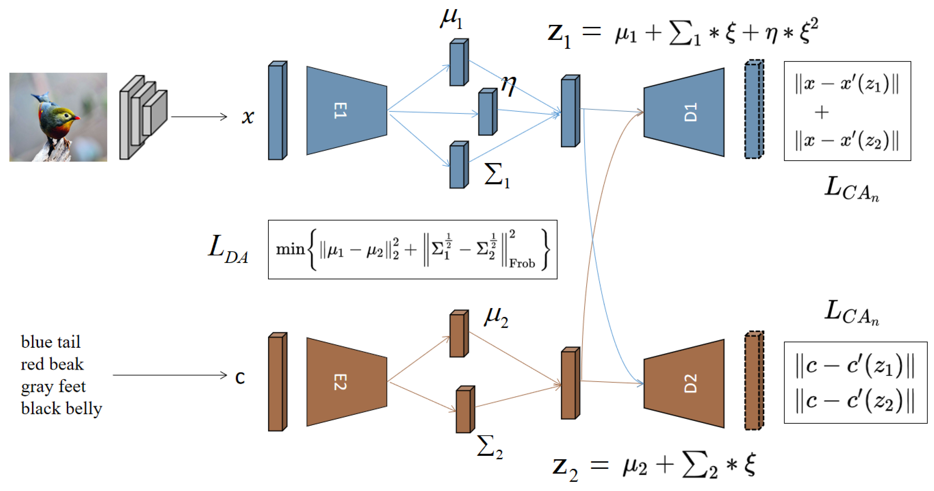
We modified the reconstruction technique to better utilize the discriminant information in visual features. We set Z 1 , and Z 2 respectively represent latent variables of the visual and semantic domain. And ξ is the random noise from the standard normal distribution which is used for increasing the generative capability of the model. The visual sample x will be encoded to μ 1 , 1 , η as it has more intrinsic discriminant information, while the semantic information c is just encodered to μ 2 , 2 like before. Then those intermediate variables will be used in the new reparametrization trick to generate respective latent distribution ( Z 1 and Z 2 ). As visible samples usually contain more information and discriminative features than semantic descriptions, we think a higher dimensional mapping function for the visual domain is more reasonable and can project visual samples to more accurate positioning in latent space and retain more discriminant information. The implicit function of Z 1 and Z 2 can be expressed respectively as:
Z 1 = μ 1 + 1 ξ + η ξ 2
Z 2 = μ 2 + 2 ξ

3.4. Model Loss

We show the basic structural details of the n-CADA-VAE in Figure 2. Our model consists of two VAE, which are used separately to process data under the visual domain (x) and semantic description (c). Each VAE consists of its encoder and decoder. Through two VAE, we can connect the information between two different modalities. We project visual feature and semantic feature to three-dimensional latent distribution ( Z 1 ) and two-dimensional latent distribution ( Z 2 ) respectively, as to better reserve the intrinsic discriminative information of the image. Latent distribution alignment is achieved by minimizing the Wasserstein distance between the latent distributions ( L D A ). Similarly, the cross-alignment loss ( L C A n ) encourages the latent distributions to align through cross-modal reconstruction [11]. The model loss function is similar to the loss function in [11], which includes cross-alignment loss ( L C A n ) and distribution-alignment loss ( L D A ), as well as basic VAE loss ( L V A E n ). The specific loss function can be expressed as:
L n C A D A V A E = δ L D A + γ L C A n + L V A E n
where δ and γ are the corresponding weighting parameters. Since the input data is just from two modalities (seen samples and semantic descriptions) in our experiment, there is only L V A E 1 and L V A E 2 loss for visual domain (x) and semantic description (c). We define the function of L V A E n as follows:
L V A E n = L V A E 1 + L V A E 2 = E q Φ ( z 1 x 1 ) log p θ ( x 1 z 1 ) β D K L q Φ ( z 1 x 1 ) | | p θ ( z 1 ) + E q Φ ( z 2 x 2 ) log p θ ( x 2 z 2 ) β D K L q Φ ( z 2 x 2 ) | | p θ ( z 2 )
The reconstruction is obtained by decoding the underlying encoding of another modal sample, in the same class. Thus, the decoder corresponding to each mode is trained based on the potential vectors of the other modalities. The distribution of different modes can also be matched with the minimum distance. Hence, the distribution-alignment loss ( L D A ) and cross-alignment loss ( L C A n ) can be defined as:
L D A = μ 1 μ 2 2 2 + Σ 1 1 2 Σ 2 1 2 F r o b e n i u s 2 1 2
L C A n = x 1 D 1 z 2 1 + x 2 D 2 z 1 1
in which D 1 and D 2 respectively represent the image feature decoder and semantic attributes decoder.

4. Experiments

4.1. Benchmark Datasets

To better contrast with CADA-VAE, we used the same datasets in our GZSL/GFSL set up to verify the performance and effectiveness of our model: including Animals with Attributes 1 and Animals with Attributes 2 (AWA1 [2], AWA2 [5]), SUN Attribute (SUN) [22] and Birds 200-2011 (CUB) [23]. SUN and CUB both have similar visual and semantic aspects as fine-grained datasets, while AWA1 and AWA2 belong to coarse-grained datasets. They are all medium-sized datasets.

4.2. Evaluation Metrics

The ZSL task, only need to identify the target in the seen and unseen classes respectively, so the Accuracy of seen ( A c c s ) and Accuracy of unseen ( A c c u ) are mainly used as indicators. However, in the GZSL task, we need to recognize samples in both visible and invisible classes at the same time, so we use their harmonic mean H as the reference of model recognition accuracy, which can be expressed as:
H = 2 A c c s A c c u A c c s + A c c u

4.3. Implementation Details

As the model we put forward is based on CADA-VAE [11], nearly all of the hyperparameters in n-CADA-VAE we continue to use the same as in CADA-VAE for a better comparison. We extract image features of 2048 dimensions for VAE training by using the pre-trained ResNet-101 model. And setting the train/test splits as in [11] to prevent violating the zero-shot assumption. The size of hidden units for the encoder and decoder of image VAE are respectively 1560 and 1660, and the encoder and decoder of attribute have 1450 and 660 hidden units. Those encoders and decoders are all Multilayer Perceptrons with one hidden layer activated by RelU. The latent embedding size for both modalities comes to 64 getting the best result.

4.4. Model Analysis on AWA1

We analyze the performance of n-CADA-VAE on AWA1 such as ablation analysis and parameter selection for the GZSL task.
Ablation Analysis. Since CADA-VAE [11] has done a similar ablation analysis, we take it as a fundamental contrast, which includes comparison results under different constraints. Not surprisingly, our approach acquires better accuracy on AWA1. And the ablation results of different constraints can be seen in Table 1.
Parameter Selection. In our experiment, the δ and γ we use are as same as in CADA-VAE [11]. We increased δ from epoch 6 to epoch 22 as well as γ from epoch 21 to 75 by a rate of 0.54 per epoch and 0.044 per epoch respectively in the experimental phase.

4.5. Comparing Approaches

In this section, we take experiment mainly on the four benchmark datasets, and compare our model n-CADA-VAE with the following models, including CVAE [21], CMT [24], SE [25], f-CLSWGAN [13], LATEM [26], SJE [27], EZSL [28], ALE [29], DeViSE [30], SYNC [31], ReViSE [32], CADA-VAE [11]. Referring to previous work [11], we compared the experimental result in the GZSL as well as the GFSL setting.
Generalized Zero-Shot Learning. The results of four benchmark datasets were shown in Table 2. Our model has a good improvement over the baseline CADA-VAE on four datasets. Compared to the baseline CADA-VAE [11], the experiments on our model gets 0.4%, 1.1%, 3.2%, and 2.1% higher accuracy on CUB, SUN, AWA1, and AWA2 respectively. Furthermore, the improvement is more obvious between data AWA1 and AWA2 we can see, as the method we put forward is more appropriate for coarse-grained datasets.
Generalized Few-Shot Learning. The same experimental steps were taken on the generalized few-shot learning as in [11], we increase the proportion of seen classes by transferring unlabeled samples to labeled, i.e., zero, one, two, five, and ten shots. The result can be seen in Figure 3, which shows our experimental results with the CADA-VAE [11] on all four datasets. And our method outperforms compared CADA-VAE for all the shot settings.

5. Conclusions

In this paper, we propose the new CADA-VAE(n-CADA-VAE) for generalized zero-shot learning and generalized few-shot learning. As the amount of information contained in data of different modalities is different (e.g., visual samples contain more feature information than the semantic description), we propose to map different modal information to different dimensional distributions of the same latent space, to make better use of the discriminant information for high-dimensional data. In the course of our experiment, we take there-dimensional and two-dimensional latent representations for the visual domain and semantic domain respectively. The most important point we propose in our paper is that we give different dimensions (weights) to the feature information in different modalities to avoid the loss caused by cross-modal embedding. The high-dimensional distribution contains more weight parameters compared to the lower dimensional distribution. So it is more suitable for storing more precise discriminative information. In this way, the loss of feature information of high-dimensional data is avoided during information transfer (information mapping). Through four benchmark datasets, we show that our model outperforms the other approaches for generalized zero-shot learning as well as few-shot learning.
More extensional research can be tried in the future, such as mapping visual features of images to higher dimensional distribution (which may be affected by specific datasets) compared to semantic information.

Author Contributions

Conceptualization, J.C. and L.W.; methodology, J.C.; validation, J.C.; formal analysis, J.L. and D.W.; supervision, X.W. and L.W. All authors have read and agreed to the published version of the manuscript.

Funding

This work was supported by the Special Fund of Advantageous and Characteristic disciplines (Group) of Hubei Province, Key R&D plan of Hubei Province (No. 2021BAA025), Industry-University-Research Innovation Fund for Chinese Universities (No. 2021FNA04004), and Open Research Fund from Guangdong Laboratory of Artificial Intelligence and Digital Economy (SZ) (No. GML-KF-22-07).

Data Availability Statement

The data included in this study are available upon request by contact with the first author ([email protected]).

Conflicts of Interest

The authors declare no conflict of interest.

References

  1. Russakovsky, O.; Deng, J.; Su, H.; Krause, J.; Satheesh, S.; Ma, S.; Huang, Z.; Karpathy, A.; Khosla, A.; Bernstein, M.; et al. Imagenet large scale visual recognition challenge. Int. J. Comput. Vis. 2015, 115, 211–252. [Google Scholar] [CrossRef] [Green Version]
  2. Lampert, C.H.; Nickisch, H.; Harmeling, S. Learning to detect unseen object classes by between-class attribute transfer. In Proceedings of the 2009 IEEE Conference on Computer Vision and Pattern Recognition, Miami, FL, USA, 20–25 June 2009; pp. 951–958. [Google Scholar]
  3. Xu, T.; Zhao, Y.; Liu, X. Dual generative network with discriminative information for generalized zero-shot learning. Complexity 2021, 2021, 6656797. [Google Scholar] [CrossRef]
  4. Chao, W.L.; Changpinyo, S.; Gong, B.; Sha, F. An empirical study and analysis of generalized zero-shot learning for object recognition in the wild. In Proceedings of the European Conference on Computer Vision, Amsterdam, The Netherlands, 11–14 October 2016; Springer: Cham, Switzerland, 2016; pp. 52–68. [Google Scholar]
  5. Xian, Y.; Lampert, C.H.; Schiele, B.; Akata, Z. Zero-shot learning—A comprehensive evaluation of the good, the bad and the ugly. IEEE Trans. Pattern Anal. Mach. Intell. 2018, 41, 2251–2265. [Google Scholar] [CrossRef] [PubMed] [Green Version]
  6. Liu, S.; Long, M.; Wang, J.; Jordan, M.I. Generalized zero-shot learning with deep calibration network. Adv. Neural Inf. Process. Syst. 2018, 31, 2009–2019. [Google Scholar]
  7. Dinu, G.; Lazaridou, A.; Baroni, M. Improving zero-shot learning by mitigating the hubness problem. arXiv 2014, arXiv:1412.6568. [Google Scholar]
  8. Shigeto, Y.; Suzuki, I.; Hara, K.; Shimbo, M.; Matsumoto, Y. Ridge regression, hubness, and zero-shot learning. In Proceedings of the Joint European Conference on Machine Learning and Knowledge Discovery in Databases, Porto, Portugal, 7–11 September 2015; Springer: Cham, Switzerland, 2015; pp. 135–151. [Google Scholar]
  9. Zhang, L.; Xiang, T.; Gong, S. Learning a deep embedding model for zero-shot learning. In Proceedings of the IEEE Conference on Computer Vision and Pattern Recognition, Honolulu, HI, USA, 21–26 July 2017; pp. 2021–2030. [Google Scholar]
  10. Huang, Y.; Deng, Z.; Wu, T. Learning discriminative latent features for generalized zero-and few-shot learning. In Proceedings of the 2020 IEEE International Conference on Multimedia and Expo (ICME), London, UK, 6–10 July 2020; pp. 1–6. [Google Scholar]
  11. Schonfeld, E.; Ebrahimi, S.; Sinha, S.; Darrell, T.; Akata, Z. Generalized zero-and few-shot learning via aligned variational autoencoders. In Proceedings of the IEEE/CVF Conference on Computer Vision and Pattern Recognition, Long Beach, CA, USA, 15–20 June 2019; pp. 8247–8255. [Google Scholar]
  12. Ni, J.; Zhang, S.; Xie, H. Dual adversarial semantics-consistent network for generalized zero-shot learning. Adv. Neural Inf. Process. Syst. 2019, 32, 6143–6154. [Google Scholar]
  13. Xian, Y.; Lorenz, T.; Schiele, B.; Akata, Z. Feature generating networks for zero-shot learning. In Proceedings of the IEEE Conference on Computer Vision and Pattern Recognition, Salt Lake City, UT, USA, 18–23 June 2018; pp. 5542–5551. [Google Scholar]
  14. Gulrajani, I.; Ahmed, F.; Arjovsky, M.; Dumoulin, V.; Courville, A.C. Improved training of wasserstein gans. Adv. Neural Inf. Process. Syst. 2017, 30, 5767–5777. [Google Scholar]
  15. Vyas, M.R.; Venkateswara, H.; Panchanathan, S. Leveraging seen and unseen semantic relationships for generative zero-shot learning. In Proceedings of the European Conference on Computer Vision, Glasgow, UK, 23–28 August 2020; Springer: Cham, Switzerland, 2020; pp. 70–86. [Google Scholar]
  16. Li, J.; Jing, M.; Lu, K.; Ding, Z.; Zhu, L.; Huang, Z. Leveraging the invariant side of generative zero-shot learning. In Proceedings of the IEEE/CVF Conference on Computer Vision and Pattern Recognition, Long Beach, CA, USA, 15–20 June 2019; pp. 7402–7411. [Google Scholar]
  17. Luo, Y.; Wang, X.; Pourpanah, F. Dual VAEGAN: A generative model for generalized zero-shot learning. Appl. Soft Comput. 2021, 107, 107352. [Google Scholar] [CrossRef]
  18. Chen, S.; Xie, G.; Liu, Y.; Peng, Q.; Sun, B.; Li, H.; You, X.; Shao, L. HSVA: Hierarchical semantic-visual adaptation for zero-shot learning. Adv. Neural Inf. Process. Syst. 2021, 34, 16622–16634. [Google Scholar]
  19. Bendre, N.; Desai, K.; Najafirad, P. Generalized zero-shot learning using multimodal variational auto-encoder with semantic concepts. In Proceedings of the 2021 IEEE International Conference on Image Processing (ICIP), Anchorage, AK, USA, 19–22 September 2021; pp. 1284–1288. [Google Scholar]
  20. Kingma, D.P.; Welling, M. Auto-encoding variational bayes. arXiv 2013, arXiv:1312.6114. [Google Scholar]
  21. Mishra, A.; Krishna Reddy, S.; Mittal, A.; Murthy, H.A. A generative model for zero shot learning using conditional variational autoencoders. In Proceedings of the IEEE Conference on Computer Vision and Pattern Recognition Workshops, Salt Lake City, UT, USA, 18–22 June 2018; pp. 2188–2196. [Google Scholar]
  22. Patterson, G.; Hays, J. Sun attribute database: Discovering, annotating, and recognizing scene attributes. In Proceedings of the 2012 IEEE Conference on Computer Vision and Pattern Recognition, Providence, RI, USA, 16–21 June 2012; pp. 2751–2758. [Google Scholar]
  23. Welinder, P.; Branson, S.; Mita, T.; Wah, C.; Schroff, F.; Belongie, S.; Perona, P. Caltech-UCSD Birds 200; Technical Report CNS-TR-2010-001; California Institute of Technology: Pasadena, CA, USA, 2010. [Google Scholar]
  24. Socher, R.; Ganjoo, M.; Manning, C.D.; Ng, A. Zero-shot learning through cross-modal transfer. Adv. Neural Inf. Process. Syst. 2013, 26, 935–943. [Google Scholar]
  25. Verma, V.K.; Arora, G.; Mishra, A.; Rai, P. Generalized zero-shot learning via synthesized examples. In Proceedings of the IEEE Conference on Computer Vision and Pattern Recognition, Salt Lake City, UT, USA, 18–23 June 2018; pp. 4281–4289. [Google Scholar]
  26. Xian, Y.; Akata, Z.; Sharma, G.; Nguyen, Q.; Hein, M.; Schiele, B. Latent embeddings for zero-shot classification. In Proceedings of the IEEE Conference on Computer Vision and Pattern Recognition, Las Vegas, NV, USA, 27–30 June 2016; pp. 69–77. [Google Scholar]
  27. Akata, Z.; Reed, S.; Walter, D.; Lee, H.; Schiele, B. Evaluation of output embeddings for fine-grained image classification. In Proceedings of the IEEE Conference on Computer Vision and Pattern Recognition, Boston, MA, USA, 7–12 June 2015; pp. 2927–2936. [Google Scholar]
  28. Romera-Paredes, B.; Torr, P. An embarrassingly simple approach to zero-shot learning. In Proceedings of the International Conference on Machine Learning, PMLR, Miami, FL, USA, 9–11 December 2015; pp. 2152–2161. [Google Scholar]
  29. Akata, Z.; Perronnin, F.; Harchaoui, Z.; Schmid, C. Label-embedding for image classification. IEEE Trans. Pattern Anal. Mach. Intell. 2015, 38, 1425–1438. [Google Scholar] [CrossRef] [PubMed] [Green Version]
  30. Frome, A.; Corrado, G.S.; Shlens, J.; Bengio, S.; Dean, J.; Ranzato, M.; Mikolov, T. Devise: A deep visual-semantic embedding model. Adv. Neural Inf. Process. Syst. 2013, 26, 2121–2129. [Google Scholar]
  31. Changpinyo, S.; Chao, W.L.; Gong, B.; Sha, F. Synthesized classifiers for zero-shot learning. In Proceedings of the IEEE Conference on Computer Vision and Pattern Recognition, Las Vegas, NV, USA, 27–30 June 2016; pp. 5327–5336. [Google Scholar]
  32. Hubert Tsai, Y.H.; Huang, L.K.; Salakhutdinov, R. Learning robust visual-semantic embeddings. In Proceedings of the IEEE International Conference on Computer Vision, Honolulu, HI, USA, 21–26 July 2017; pp. 3571–3580. [Google Scholar]
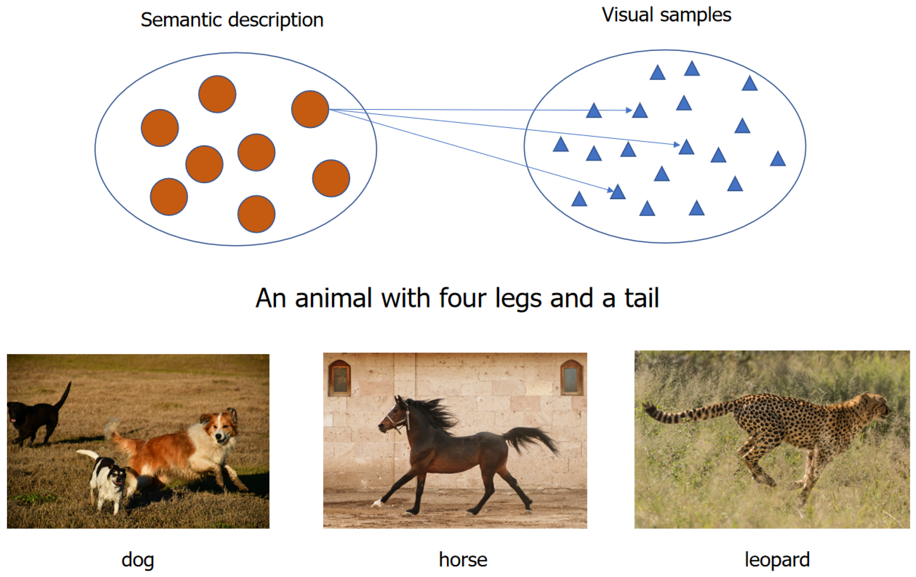
Figure 1. An illustration of visual samples contains more feature information than the semantic description (e.g., sentence, attribute, and word2vec embeddings).
Information 14 00148 g001
Figure 2. The proposed new CADA-VAE(n-CADA-VAE) model.
Information 14 00148 g002
Figure 3. The comparison of our model and CADA-VAE with different proportions of training samples from unseen classes in the GFSL.
Information 14 00148 g003
Table 1. Ablation study of GZSL based under different settings in the Ablation study on dataset AWA1.
ModelSUH
DA-VAE65.160.162.5
CA-VAE61.356.558.8
CADA-VAE72.857.364.1
n-CADA-VAE74.661.367.3
Table 2. The results of GZSL were compared mainly with CADA-VAE. Containing seen (S) classes, unseen (U) classes, and their harmonic mean (H).
MethodsCUBSUNAWA1AWA2
SUHSUHSUHSUH
CMT [24] 49.87.212.621.88.111.887.60.91.890.00.51.0
SJE [27] 59.223.533.630.514.719.874.611.319.673.98.014.4
ALE [29] 62.823.734.433.121.826.376.116.827.581.814.023.9
LATEM [26] 57.315.224.028.814.719.571.77.313.377.311.520.0
EZSL [28] 63.812.621.027.911.015.875.66.612.177.85.911.0
SYNC [31] 70.911.519.843.37.913.487.38.916.290.510.018.0
DeViSE [30] 53.023.832.827.416.920.968.713.422.474.717.127.8
f-CLSWGAN [13] 57.743.749.736.642.639.461.457.959.668.952.159.4
SE [25] 53.341.546.730.540.934.967.856.361.568.158.362.8
ReViSE [32] 28.337.632.320.124.322.037.146.141.139.746.442.8
CADA-VAE [11] 53.551.652.435.747.240.672.857.364.175.055.863.9
n-CADA-VAE54.751.052.835.750.141.774.661.367.378.657.066.0
Disclaimer/Publisher’s Note: The statements, opinions and data contained in all publications are solely those of the individual author(s) and contributor(s) and not of MDPI and/or the editor(s). MDPI and/or the editor(s) disclaim responsibility for any injury to people or property resulting from any ideas, methods, instructions or products referred to in the content.