Multi-Target Rough Sets and Their Approximation Computation with Dynamic Target Sets

Abstract

Multi-label learning has become a hot topic in recent years, attracting scholars’ attention, including applying the rough set model in multi-label learning. Exciting works that apply the rough set model into multi-label learning usually adapt the rough sets model’s purpose for a single decision table to a multi-decision table with a conservative strategy. However, multi-label learning enforces the rough set model which wants to be applied considering multiple target concepts, and there is label correlation among labels naturally. For that proposal, this paper proposes a rough set model that has multiple target concepts and considers the similarity relationships among target concepts to capture label correlation among labels. The properties of the proposed model are also investigated. The rough set model that has multiple target concepts can handle the data set that has multiple decisions, and it has inherent advantages when applied to multi-label learning. Moreover, we consider how to compute the approximations of GMTRSs under a static and dynamic situation when a target concept is added or removed and derive the corresponding algorithms, respectively. The efficiency and validity of the designed algorithms are verified by experiments.

1. Introduction

Rough set theory, which is proposed by Pawlak [1], has been widely applied in multiple popular aspects, including classification [2,3], clustering [4], feature selection and attribute reduction [5]. Based on different types of generalizations of the rough set model, lots of works have been introduced. For example, some extended models based on the neighborhood have been discussed and applied to medical lung cancer disease [6]. At the same time, soft β-rough sets have been applied in determining COVID-19 [7]. Some models have also been used in clustering [4,8]. Rough set theory can also be used for feature selection [9,10] and could be comparable with some state-of-the-art methods.

These works deal with the learning paradigm called single-label learning or classic machine learning [11], in which the learning task has only one label or decision. This learning paradigm suffers great limitations in that real-life application usually has multiple labels. For overcoming the defect of single-label learning, Zhang et al. [12] proposed a multi-label learning paradigm. It is a powerful learning paradigm that is more suitable for real-life learning. After multi-label learning was proposed, rough set theories were applied in the learning paradigm [13,14] but mainly applied in multi-label feature selection.

Decided by the type of rough set model the paper uses, these works could mainly be categorized into: (1) Classical rough sets or Pawlak rough sets. For example, based on the concept of positive region, Li et al. [14] proposed a feature selection method for multi-label learning. Chen et al. [15] proposed a dynamic way for updating decision rules based on rough sets. (2) Neighborhood rough sets. For example, by reconstructing the lower approximation and its corresponding positive region, Duan et al. [16] proposed a feature selection approach for multi-label learning. Online multi-label feature selections, which are neighborhood rough set models were also considered by Liu et al. [17]. There is some similar work such as [18,19,20]. (3) Fuzzy rough sets, including fuzzy rough sets [21,22,23,24], kernelized fuzzy rough sets [25,26], fuzzy neighborhood rough sets [27] and so on. No matter what model these works use, they are all trying to adapt a type of rough set model to a multi-label learning paradigm. Eventually, the models they use were designed for single-label learning, which means they have only one target concept. Authors either made some modifications to the basic concept of positive region or transferred the multi-label problem into a single-label one.

But in multi-label learning, there are multiple decisions compared to single-label learning. Pawlak’s rough sets model and its extended models are all designed for single-label learning, which means they may have some limitations when they are applied in a multi-label decision information system. For example, by extending the classical rough set model into a multi-label scenario, Li et al. [14] proposed an attribute reduction approach for multi-label learning. This kind of work has two limitations: (1) They treat all the labels the same. They either calculate the union of approximation for a single decision or their intersect. Some labels only associated with a few instances will lead to a weak result when we use such a strategy. (2) Label correlation among multi-labels is ignored. Labels have their own clusters; some labels usually appear with some specific labels, while some specific labels do not. Using a conservative or liberal strategy to organize multiple labels will ignore all label correlation among labels because they assume all the labels have equal levels, which is not appropriate. To overcome these drawbacks of a traditional rough set model, we try to propose a novel multi-target rough set model so that the model can be easily used in a multi-label decision information system. The targets in the target group are organized by the similarity measure because the label correlation does exist among labels [28]. Thus, we can use the label correlation measure to organize targets naturally.

In rough set theory, calculating the approximations is an old, classic but important problem. In recent years, the computational and updating of multi-granular coarse sets and their extended models have attracted great attention from many researchers. These studies are usually divided into four categories according to the change scenarios in the data sets: increasing or decreasing attributes [29,30,31,32], changing attribute values [15], changing decision attributes [33] and changing object set changes [34]. The approximation computation of our proposed model can boost the process of decision making or attribute reduction approaches, for it is more efficient than directly calculating the approximation via set operation. After the model is given, here we try to consider how to compute the approximations of our proposed model. We propose an approach for calculating the approximations for the model’s future applications and also consider the properties of the approximations when a target concept is added or removed. According to the properties we discuss, the corresponding approximation computation algorithms are designed. All the algorithms’ effectiveness and efficiency are valid by experiments. The difference between our model and existing relative models is our GMTRS considers the target set with lots of targets and considers the correlation or relation among the targets. First, there are few rough sets models which consider that the target could be a set group. Furthermore, for considering the correlation among the targets, the model can be used for addressing problems in multi-label learning or other scenarios.

The contributions of this paper are as follows:

• A rough set model considering the label correlation is proposed for multi-label learning. It provides a novel approach for handling multi-label information systems.
• The properties of the proposed models are investigated in this paper.
• An algorithm for calculating the approximations in the proposed rough set model is designed in this paper. It will boost the application of the proposed multi-target rough set model.
• Two algorithms for calculating the approximations in the proposed rough set model under the situation of adding (removing) a target concept to (from) the target group are proposed in this paper. It will improve the efficiency of calculating the approximations of the proposed model.
• Experiments are conducted to validate the efficiency and effectiveness of all proposed algorithms.

The rest of this paper is organized as follows. Some basic concepts of GMTRSs are introduced, and their properties are discussed in Section 2. In Section 3, we consider the computation of the approximations of GMTRSs, and we further discuss the situations of adding and removing a target concept in Section 4, respectively. All the algorithms are evaluated in Section 5. Finally, we conclude the whole paper with Section 6.

2. Global Multi-Target Rough Sets

In this section, some concepts associated with our proposed model are introduced and then the properties of the proposed model are discussed.

2.1. Definitions

In this subsection, the definitions of several multi-target rough sets are introduced.

Definition 1

([35]). (set correlation, SC) Suppose $U$ is a finite universe,$\left(U,A\right)$ is an information system and $X=\left\{X_1,X_2,\cdots ,X_r\right\}$ is a finite target set which satisfies, for all $X_i\in X,X_i\subseteq U.$ Then the correlation is defined as

$$\begin{gathered} S_R(X_i,X_j)=\frac{\left|X_i\cap X_j\right|}{\left|X_i\right|},i,j\le r(\mathit{relative}\mathit{correlation}); \\ {S}_A(X_i,X_j)=\frac{\left|X_i\cap X_j\right|}{\left|X_i\cup X_j\right|},i,j\le r(\mathit{absolute}\mathit{correlation}). \end{gathered}$$

Definition 2.

(global correlated target set, GCTS) Suppose $U$is a finite universe,$\left(U,A\right)$is an information system and$X=\left\{X_1,X_2,\cdots ,X_r\right\}$is a finite target set which satisfies, for all$X_i\in X,X_i\subseteq U.$Then$\mathit{X}$is a global correlated target set if, for all$X_i$,there exists$X_j$,such that$S_R\left(X_i,X_j\right)>\alpha$and$S_R\left(X_j,X_i\right)>\alpha$. Here,$\alpha \in \left(0,1\right]$is the correlation control parameter (CCP) among targets, and it controls the similarity degree among the targets in the target group.

The GCTS is a target group in which any target set has its partner that meets the correlation condition. It is not pairwise correlated; the condition of the GCTS is looser than pairwise correlated. It provides an effective way for capturing and using label correlation in rough set theory.

Relatively, there is a local correlated target set.

Definition 3.

(local correlated target set, LCTS) Suppose $U$is a finite universe,$\left(U,A\right)$is an information system and$X=\left\{X_1,X_2,\cdots ,X_r\right\}$is a finite target set which satisfies, for all$X_i\in X,X_i\subseteq U.$Then$X$is a local correlated target set if and only if, for all$X_i\in X$,thereexists$X_j\in X$, such that$S_R\left(X_i,X_j\right)>\alpha$.

Based on the definition of the GCTS and Pawlak’s rough sets, we can define a global multi-target rough set accordingly.

Definition 4.

(global multi-target rough set, GMTRS) Suppose$U$is a finite universe,$\left(U,A\right)$is an information system and$X=\left\{X_1,X_2,\cdots ,X_r\right\}$is a GCTS.

Then the lower approximation of a GMTRS is defined as

$${\underset{¯}{R}}_G(\mathit{X})=\{x\in U{\left|[x]\right.}_A\subseteq X_1\wedge {[x]}_A\subseteq X_2\wedge \cdots \wedge {[x]}_A\subseteq X_r\}.$$

The upper approximation of a GMTRS is defined as

$${\overline{R}}_G(\mathit{X})=\{x\in U{\left|[x]\right.}_A\cap X_1\ne \varphi \vee {[x]}_A\cap X_2\ne \varphi \vee \cdots \vee {[x]}_A\cap X_r\ne \varphi \}.$$

With the help of the CCP, we can organize different targets together. The lower approximation is a conservative approximation of the target group which needs all the targets to meet the same condition. Relatively, the upper approximation obeys a liberal strategy, only needing one target of the target group to meet the condition.

Example 1.

A multi-label decision information system is as follows: It has two labels which are assumed to be two different target concepts. We can easily obtain that when α = 0.4 the target group is a GCTS. For clarifying the definition of a GMTRS, we have an example for a GMTRS. Since

$X_1=\left\{x_2,x_3,x_5\right\},X_2=\left\{x_1,x_2,x_5\right\},\alpha =0.4,S_R\left(X_1,X_2\right)=2/3>0.4=\alpha .$

FromTable 1, we have${\left[x_1\right]}_A=\left\{x_1\right\},{\left[x_2\right]}_A={\left[x_5\right]}_A=\left\{x_2,x_5\right\},{\left[x_3\right]}_A=\left\{x_3\right\},{\left[x_4\right]}_A=\left\{x_4\right\}.$

From Definition 4, we have${\left[x_1\right]}_A=\left\{x_1\right\}\not\subset X_1\wedge {\left[x_1\right]}_A\subseteq X_2,{\left[x_2\right]}_A\subseteq X_1\wedge {\left[x_2\right]}_A\subseteq X_2,$

${\left[x_3\right]}_A\subseteq X_1\wedge {\left[x_3\right]}_A\not\subset X_2,{\left[x_4\right]}_A{X}_1\wedge {\left[x_4\right]}_A\not\subset X_2,{\left[x_5\right]}_A\subseteq X_1\wedge {\left[x_5\right]}_A\subseteq X_2.$

Thus, we have${\underset{\_}{R}}_G\left(\mathit{X}\right)=\left\{x_2,x_5\right\}.$

From Definition 4, we have${\left[x_1\right]}_A\cap X_2\ne \varphi ,{\left[x_2\right]}_A\cap X_1\ne \varphi ,{\left[x_3\right]}_A\cap X_1\ne \varphi ,{\left[x_5\right]}_A\cap X_1\ne \varphi ,$

${\left[x_4\right]}_A\cap X_1=\varphi \wedge {\left[x_4\right]}_A\cap X_2=\varphi , \text{Thus, we have}{\overline{R}}_G(\mathit{X})=\left\{x_1,x_2,x_3,x_5\right\}.$

Table 1. An example of multi-label table.

U	a1	a2	a3	X1	X2
x1	1	M	1	0	1
x2	2	F	2	1	1
x3	2	M	2	1	0
x4	1	M	2	0	0
x5	2	F	2	1	1

Table 1. An example of multi-label table.

U	a1	a2	a3	X1	X2
x1	1	M	1	0	1
x2	2	F	2	1	1
x3	2	M	2	1	0
x4	1	M	2	0	0
x5	2	F	2	1	1

2.2. Properties

The properties of GMTRSs are discussed in this subsection.

Proposition 1.

Suppose $U$is a finite universe,$\left(U,A\right)$is an information system and$X=\left\{X_1,X_2,\cdots ,X_r\right\}$is a GCTS. For the approximations of a GMTRS:

• Forall $X_i\in X,X_i=U$if and only if${\underset{\_}{R}}_G\left(X\right)=U$;
• There exists $X_i\in X,X_i=U$if and only if ${\overline{R}}_G\left(X\right)=U$;
• There exists $X_i\in X,X_i=\varphi$if and only if ${\underset{\_}{R}}_G\left(X\right)=\varphi$;
• Forall $X_i\in X,X_i=\varphi$if and only if ${\overline{R}}_G\left(X\right)=\varphi$.

Proof.

• For all $X_i\in X,X_i=U$ implies, for all $x\in U$, for all $i\in \left\{1,2,\cdots ,r\right\},{\left[x\right]}_A\subseteq X_i$, which implies ${\left[x\right]}_A\subseteq X_1\wedge {\left[x\right]}_A\subseteq X_2\wedge \cdots \wedge {\left[x\right]}_A\subseteq X_r$ if and only if $x\in {\underset{\_}{R}}_G\left(\mathit{X}\right)$, so ${\underset{\_}{R}}_G\left(X\right)=U$;
• There exists $X_i\in X,X_i=U$, which implies, for all $x\in U$, that there exists $i\in \left\{1,2,\cdots ,r\right\},{\left[x\right]}_A\cap X_i\ne \varphi$, which implies ${\left[x\right]}_A\cap X_1\ne \varphi \vee \cdots \vee {\left[x\right]}_A\cap X_r\ne \varphi$ if and only if $x\in {\overline{R}}_G\left(X\right)$, so ${\overline{R}}_G\left(X\right)=U$;
• There exists $X_i\in X,X_i=\varphi$, which implies, for all $x\in U$, that there exists $i\in \left\{1,2,\cdots ,r\right\},{\left[x\right]}_A\not\subset X_i$ which implies $x\notin {\underset{\_}{R}}_G\left(X\right)$, so ${\underset{\_}{R}}_G\left(X\right)=\varphi$;
• For all $X_i\in X,X_i=\varphi$ implies, for all $x\in U$, for all $i\in \left\{1,2,\cdots ,r\right\},{\left[x\right]}_A\cap X_i=\varphi$, which implies $x\notin {\overline{R}}_G\left(X\right)$, so ${\overline{R}}_G\left(X\right)=\varphi$.□

Proposition 2.

Suppose $U$is a finite universe,$\left(U,A\right)$is an information system and$X=\left\{X_1,X_2,\cdots ,X_r\right\}$is a GCTS. For the approximations of a GMTRS:

• For all$X_i\in X,{\underset{\_}{R}}_G\left(X\right)\subseteq X_i$;
• For all$X_i\in X,X_i\subseteq {\overline{R}}_G\left(X\right)$.

Proof. 

• For all $x\in {\underset{\_}{R}}_G\left(X\right)$, it is implied that ${\left[x\right]}_A\subseteq X_i$ if and only if ${\left[x\right]}_A\subseteq X_1\wedge {\left[x\right]}_A\subseteq X_2\wedge \cdots \wedge {\left[x\right]}_A\subseteq X_r$, which implies for all $i\in \left\{1,2,\cdots ,r\right\},x\subseteq X_i$, so ${\underset{\_}{R}}_G\left(X\right)\subseteq X_i$.
• For all $x\in X_i$, it is implied that there exists $i\in \left\{1,2,\cdots ,r\right\},{\left[x\right]}_A\cap X_i=\varphi$, which implies $x\in {\overline{R}}_G\left(X\right)$, so $X_i\subseteq {\overline{R}}_G\left(X\right)$. □

Proposition 3.

Suppose$U$is a finite universe,$\left(U,A\right)$is an information system $Z=\left\{Z_1,Z_2,\cdots ,Z_r\right\}$is a GCTS and $\mathit{X},\mathit{Y}\subseteq \mathit{Z}$. For the approximations of a GMTRS:

• ${\underset{\_}{R}}_G\left(X\cap Y\right)\supseteq {\underset{\_}{R}}_G\left(X\right)\cap {\underset{\_}{R}}_G\left(Y\right)$;
• ${\overline{R}}_G\left(X\cap Y\right)\subseteq {\overline{R}}_G\left(X\right)\cap {\overline{R}}_G\left(Y\right)$;
• ${\underset{\_}{R}}_G\left(X\cup Y\right)\subseteq {\underset{\_}{R}}_G\left(X\right)\cup {\underset{\_}{R}}_G\left(Y\right)$;
• ${\overline{R}}_G\left(X\cup Y\right)={\overline{R}}_G\left(X\right)\cup {\overline{R}}_G\left(Y\right)$.

Proof. 

• For all $x\in {\underset{\_}{R}}_G\left(X\right)\cap {\underset{\_}{R}}_G\left(Y\right)$, it is implied that, for all $X_i\in X\left(i\le \left|X\right|\right),{\left[x\right]}_A\subseteq X_i$ and, for all $Y_j\in Y\left(j\le \left|Y\right|\right),{\left[x\right]}_A\subseteq Y_j$, which implies, for all $Z_k\in X\cap Y\left(k\in \left\{1,2,\cdots ,r\right\}\right),{\left[x\right]}_A\subseteq Z_k$ if and only if $x\in {\underset{\_}{R}}_G\left(X\cap Y\right)$, so ${\underset{\_}{R}}_G\left(X\cap Y\right)\supseteq {\underset{\_}{R}}_G\left(X\right)\cap {\underset{\_}{R}}_G\left(Y\right)$;
• For all $x\in {\overline{R}}_G\left(X\cap Y\right)$, $x\in {\overline{R}}_G\left(X\cap Y\right)$ if and only if there exists $Z_k\in X\cap Y\left(k\in \left\{1,2,\cdots ,r\right\}\right),{\left[x\right]}_A\cap Z_k\ne \varphi$, which implies there exists $X_i\in X\left(i\le \left|X\right|\right),{\left[x\right]}_A\cap X_i\ne \varphi$ and there exists $Y_j\in Y\left(j\le \left|Y\right|\right),{\left[x\right]}_A\cap Y_j\ne \varphi$, which implies $x\in {\overline{R}}_G\left(X\right)\cap {\overline{R}}_G\left(Y\right)$, so ${\overline{R}}_G\left(X\cap Y\right)\subseteq {\overline{R}}_G\left(X\right)\cap {\overline{R}}_G\left(Y\right);$
• For all $x\in {\underset{\_}{R}}_G\left(X\cup Y\right)$, $x\in {\underset{\_}{R}}_G\left(X\cup Y\right)$ if and only if, for all $Z_k\in X\cup Y\left(k\in \left\{1,2,\cdots ,r\right\}\right),{\left[x\right]}_A\subseteq Z_k$, which implies, for all $X_i\in X\left(i\le \left|X\right|\right),{\left[x\right]}_A\subseteq X_i$ or, for all $Y_j\in Y\left(j\le \left|Y\right|\right),{\left[x\right]}_A\subseteq Y_j$, which implies $x\in {\underset{\_}{R}}_G\left(X\right) \text{or} x\in {\underset{\_}{R}}_G\left(Y\right),$ which implies $x\in \left({\underset{\_}{R}}_G\left(X\right)\cup {\underset{\_}{R}}_G\left(Y\right)\right),$ so ${\underset{\_}{R}}_G\left(X\cup Y\right)\subseteq {\underset{\_}{R}}_G\left(X\right)\cup {\underset{\_}{R}}_G\left(Y\right)$;
• For all $x\in {\overline{R}}_G\left(X\cup Y\right)$, if and only if there exists $Z_k\in X\cup Y\left(k\in \left\{1,2,\cdots ,r\right\}\right),{\left[x\right]}_A\cap Z_k\ne \varphi$, if and only if there exists $X_i\in X\left(i\le \left|X\right|\right),{\left[x\right]}_A\cap X_i\ne \varphi$ or there exists $Y_j\in Y\left(j\le \left|Y\right|\right),{\left[x\right]}_A\cap Y_j\ne \varphi$, which implies $x\in {\overline{R}}_G\left(X\right) \text{or} x\in {\overline{R}}_G\left(Y\right),$ if and only if ${\overline{R}}_G\left(X\cup Y\right)={\overline{R}}_G\left(X\right)\cup {\overline{R}}_G\left(Y\right)$.□

Proposition 4.

Suppose $U$is a finite universe,$\left(U,A\right)$is an information system,$Z=\left\{Z_1,Z_2,\cdots ,Z_r\right\}$is a GCTS and$X\subseteq Y\subseteq Z$. For the approximations of a GMTRS:

• ${\underset{\_}{R}}_G\left(X\right)\supseteq {\underset{\_}{R}}_G\left(Y\right)$;
• ${\overline{R}}_G\left(X\right)\subseteq {\overline{R}}_G\left(Y\right)$.

Proof. 

• For all $x\in {\underset{\_}{R}}_G\left(Y\right)$, if and only if, for all $Z_k\in Y,k\in \left\{1,2,\cdots ,r\right\},{\left[x\right]}_A\subseteq Z_k,$ which implies for all $Z_k\in X,k\in \left\{1,2,\cdots ,r\right\},{\left[x\right]}_A\subseteq Z_k,$ which implies $x\in {\underset{\_}{R}}_G\left(X\right)$ so ${\underset{\_}{R}}_G\left(X\right)\supseteq {\underset{\_}{R}}_G\left(Y\right)$.
• For all $x\in {\overline{R}}_G\left(X\right)$, if and only if there exists $Z_k\in X,k\in \left\{1,2,\cdots ,r\right\},{\left[x\right]}_A\cap Z_k\ne \varphi$, which implies there exists $Z_k\in Y,k\in \left\{1,2,\cdots ,r\right\},{\left[x\right]}_A\cap Z_k\ne \varphi$ which implies $x\in {\overline{R}}_G\left(Y\right),$ so ${\overline{R}}_G\left(X\right)\subseteq {\overline{R}}_G\left(Y\right)$. □

3. Approximation Computation of GMTRSs

In this section, we propose an approach for computing the approximations of GMTRSs. We induce some corresponding results for approximation computation and then design an algorithm for calculating the approximations of GMTRSs.

Definition 5

([35]). Suppose $U$ is a finite universe, $P\subseteq U$ and the matrix representation of set $P$ is defined as:

$$\overrightarrow{P}={\left(p_j\right)}_{n\times 1},j\in \left\{1,2,\cdots ,n\right\},n=\left|U\right|\mathrm{where}{p}_j=\left\{\begin{array}{cc}0\hfill & x_j\notin P\\ 1\hfill & x_j\in P\end{array}\right..$$

(1)

Example 2.

Continuation of Example 1. By Definition 5, we have

${\overrightarrow{\left[x_1\right]}}_A={\left(1,0,0,0,0\right)}^{\prime },{\overrightarrow{\left[x_2\right]}}_A={\overrightarrow{\left[x_5\right]}}_A={\left(0,1,0,0,1\right)}^{\prime },{\overrightarrow{\left[x_3\right]}}_A={\left(0,0,1,0,0\right)}^{\prime },$

${\overrightarrow{\left[x_4\right]}}_A={\left(0,0,0,1,0\right)}^{\prime }.$Here,${\overrightarrow{M}}^{\prime }$means the transpose of matrix$\overrightarrow{M}$.

Lemma 1.

Suppose$X,Y\subseteq U.$We have:

• $X\cap Y\ne \varphi \iff {\overrightarrow{X}}^{\prime }\cdot \overrightarrow{Y}>0$;
• $X\subseteq Y\iff {\overrightarrow{X}}^{\prime }\cdot \overrightarrow{\sim Y}=0$.

Here,$\sim Y$is a complement of$Y$,${\overrightarrow{X}}^{\prime }$means the transpose of matrix$\overrightarrow{X}$, and ‘$\cdot$’ is the matrix quantity product.

There is a useful property about computing the approximations of GMTRSs using Lemma 1.

Theorem 1.

Suppose$U$is a finite universe,$\left(U,A\right)$is an information system and$X$is a GCTS. We have:

• $x\in {\underset{\_}{R}}_G\left(X\right)\iff \forall i\in \left\{1,2,\cdots ,r\right\},{\overrightarrow{\left[x\right]}}_A^{\prime }\cdot \overrightarrow{\sim X_i}=0$;
• $x\in {\overline{R}}_G\left(X\right)\iff \exists i\in \left\{1,2,\cdots ,r\right\},{\overrightarrow{\left[x\right]}}_A^{\prime }\cdot \overrightarrow{X_i}>0$.

Proof. 

From Lemma 1,

• For all $i\in \left\{1,2,\cdots ,r\right\},{\overrightarrow{\left[x\right]}}_A^{\prime }\cdot \overrightarrow{\sim X_i}=0,$ if and only if, for all $i\in \left\{1,2,\cdots ,r\right\},{\left[x\right]}_A\subseteq X_i,$ if and only if $x\in {\underset{\_}{R}}_G\left(X\right)$;
• There exists $i\in \left\{1,2,\cdots ,r\right\},{\overrightarrow{\left[x\right]}}_A^{\prime }\cdot \overrightarrow{X_i}>0$ if and only if there exists $i\in \left\{1,2,\cdots ,r\right\},{\left[x\right]}_A\cap X_i\ne \varphi ,$ if and only if $x\in {\overline{R}}_G\left(X\right)$. □

The matrix representation of Theorem 1 is as the following two definitions.

Definition 6.

Suppose$U$is a finite universe,$\left(U,A\right)$is an information system and$X$is a GCTS. Then the lower approximation matrix of a GMTRS can be defined as

$$\underset{\_}{H}\left(X\right)={\left({\underset{\_}{h}}_{ij}\right)}_{r\times n},\mathrm{where}{\underset{\_}{h}}_{ij}=\{\begin{array}{cc}1\hfill & {\overrightarrow{\left[x_j\right]}}_A^{\prime }·\overrightarrow{\sim X_i}=0\hfill \\ 0\hfill & otherwise\hfill \end{array} i\in \left\{1,2,\cdot \cdot \cdot ,r\right\},j\in \left\{1,2,\cdot \cdot \cdot ,n\right\};$$

(2)

and the upper approximation matrix of a GMTRS can be defined as

$$\overline{H}\left(X\right)={\left({\overline{h}}_{ij}\right)}_{r\times n},\mathrm{where}{\bar{h}}_{ij}=\{\begin{array}{cc}1\hfill & {\overrightarrow{\left[x_j\right]}}_A^{\prime }\cdot \overrightarrow{X_i}>0\hfill \\ 0\hfill & otherwise\hfill \end{array}i\in \left\{1,2,\cdot \cdot \cdot ,r\right\},j\in \left\{1,2,\cdot \cdot \cdot ,n\right\}.$$

(3)

Example 3.

Continuation of Example 2. By Definition 5, we have

$\overrightarrow{X_1}={\left(0,1,1,0,1\right)}^{\prime },\overrightarrow{\sim X_1}={\left(1,0,0,1,0\right)}^{\prime },\overrightarrow{X_2}={\left(1,1,0,0,1\right)}^{\prime },\overrightarrow{\sim X_2}={\left(0,0,1,1,0\right)}^{\prime }.$

By Definition 6, we have

${\overrightarrow{\left[x_1\right]}}_A^{\prime }\cdot \overrightarrow{\sim X_1}=\left(1,0,0,0,0\right)\cdot {\left(1,0,0,1,0\right)}^{\prime }\ne 0,{\overrightarrow{\left[x_1\right]}}_A^{\prime }\cdot \overrightarrow{\sim X_2}=0;$

${\overrightarrow{\left[x_2\right]}}_A^{\prime }\cdot \overrightarrow{\sim X_1}=0,{\overrightarrow{\left[x_2\right]}}_A^{\prime }\cdot \overrightarrow{\sim X_2}=0;{\overrightarrow{\left[x_3\right]}}_A^{\prime }\cdot \overrightarrow{\sim X_1}=0,{\overrightarrow{\left[x_3\right]}}_A^{\prime }\cdot \overrightarrow{\sim X_2}\ne 0;$

${\overrightarrow{\left[x_4\right]}}_A^{\prime }\cdot \overrightarrow{\sim X_1}\ne 0,{\overrightarrow{\left[x_4\right]}}_A^{\prime }\cdot \overrightarrow{\sim X_2}\ne 0;{\overrightarrow{\left[x_5\right]}}_A^{\prime }\cdot \overrightarrow{\sim X_1}=0,{\overrightarrow{\left[x_5\right]}}_A^{\prime }\cdot \overrightarrow{\sim X_2}=0;$

Thus, we have $\underset{\_}{H}\left(X\right)=\left(\begin{array}{ccccc}0& 1& 1& 0& 1\\ 1& 1& 0& 0& 1\end{array}\right).$

Example 4.

Continuation of Example 3. By Definition 6, we have

${\overrightarrow{\left[x_1\right]}}_A^{\prime }\cdot \overrightarrow{X_1}=\left(1,0,0,0,0\right)\cdot {\left(0,1,1,0,1\right)}^{\prime }=0,{\overrightarrow{\left[x_1\right]}}_A^{\prime }\cdot \overrightarrow{X_2}>0;$

${\overrightarrow{\left[x_2\right]}}_A^{\prime }\cdot \overrightarrow{X_1}>0,{\overrightarrow{\left[x_2\right]}}_A^{\prime }\cdot \overrightarrow{X_2}>0;{\overrightarrow{\left[x_3\right]}}_A^{\prime }\cdot \overrightarrow{X_1}>0,{\overrightarrow{\left[x_3\right]}}_A^{\prime }\cdot \overrightarrow{X_2}=0;$

${\overrightarrow{\left[x_4\right]}}_A^{\prime }\cdot \overrightarrow{X_1}=0,{\overrightarrow{\left[x_4\right]}}_A^{\prime }\cdot \overrightarrow{X_2}=0;{\overrightarrow{\left[x_5\right]}}_A^{\prime }\cdot \overrightarrow{X_1}>0,{\overrightarrow{\left[x_5\right]}}_A^{\prime }\cdot \overrightarrow{X_2}>0;$

Thus, we have$\overline{H}\left(X\right)=\left(\begin{array}{ccccc}0& 1& 1& 0& 1\\ 1& 1& 0& 0& 1\end{array}\right).$

Then we can easily obtain a theorem for computing approximations in GMTRSs.

Theorem 2.

Suppose$U$is a finite universe,$\left(U,A\right)$is an information system and Xis a GCTS. We have:

• $x_j\in {\underset{\_}{R}}_G\left(X\right)\iff {\wedge }_{i=1}^r{\underset{\_}{h}}_{ij}=1;$
• $x_j\in {\overline{R}}_G\left(X\right)\iff {\vee }_{i=1}^r{\overline{h}}_{ij}=1.$

Proof. 

From Lemma 1,

• $x_j\in {\underset{\_}{R}}_G\left(X\right)$ if and only if for all $i\in \left\{1,2,\cdots ,r\right\},{\overrightarrow{\left[x_j\right]}}_A^{\prime }\cdot \overrightarrow{\sim X_i}=0$, if and only if, for all $i\in \left\{1,2,\cdots ,r\right\},{\underset{\_}{h}}_{ij}=1,$ if and only if ${\wedge }_{i=1}^r{\underset{\_}{h}}_{ij}=1;$
• $x_j\in {\overline{R}}_G\left(X\right)$ if and only if there exists $i\in \left\{1,2,\cdots ,r\right\},{\overrightarrow{\left[x_j\right]}}_A^{\prime }\cdot \overrightarrow{X_i}>0$ , if and only if there exists $i\in \left\{1,2,\cdots ,r\right\},{\overline{h}}_{ij}=1,$ if and only if ${\vee }_{i=1}^r{\overline{h}}_{ij}=1.$□

Example 5.

Continuation of Examples 3 and 4. By Theorem 2, we have

$\overrightarrow{{\underset{\_}{R}}_G\left(X\right)}={\left(0,1,1,0,1\right)}^{\prime }\wedge {\left(1,1,0,0,1\right)}^{\prime }={\left(0,1,0,0,1\right)}^{\prime };$

$\overrightarrow{{\overline{R}}_G\left(X\right)}={\left(0,1,1,0,1\right)}^{\prime }\vee {\left(1,1,0,0,1\right)}^{\prime }={\left(1,1,1,0,1\right)}^{\prime }.$

Thus,${\underset{\_}{R}}_G\left(\mathit{X}\right)=\left\{x_2,x_5\right\},{\overline{R}}_G\left(\mathit{X}\right)=\left\{x_1,x_2,x_3,x_5\right\}.$

Based on Theorem 2, we propose matrix-based Algorithm 1 for computing the approximations of a particular target concept group. The total time complexity of Algorithm 1 is $\Theta \left(r{n}^2\right).$ Lines 2–15 are to calculate $\overline{H}$ and $\underset{\_}{H}$ with time complexity $\Theta \left(r{n}^2\right).$

Algorithm 1. Computing Approximations of GMTRSs (CAG).
Input: $\left(U,A\right),X=\left\{X_1,X_2,\cdots ,X_r\right\},{\left[x\right]}_A$
Output:${\overline{R}}_G\left(X\right),{\underset{\_}{R}}_G\left(X\right)$
1:	$n\leftarrow \left|U\right|,r\leftarrow \left|X\right|$
2:	for $i=1\to r$
3:	for$j=1\to n$
4:	if${\overrightarrow{\left[x_j\right]}}_A^{\prime }\cdot \overrightarrow{\sim X_i}=0$then
5:	${\underset{\_}{h}}_{ij}=1$
6:	else
7:	${\underset{\_}{h}}_{ij}=0$
8:	end if
9:	if${\overrightarrow{\left[x_j\right]}}_A^{\prime }\cdot \overrightarrow{X_i}>0$then
10:	${\overline{h}}_{ij}=1$
11:	else
12:	${\overline{h}}_{ij}=0$
13:	end if
14:	end for
15:	end for
16:	$\overrightarrow{{\underset{\_}{R}}_G\left(X\right)}={\left({\wedge }_{i=1}^r{\underset{\_}{h}}_{i\ast }\right)}^{\prime }={\left({\wedge }_{i=1}^r{\underset{\_}{h}}_{i1},{\wedge }_{i=1}^r{\underset{\_}{h}}_{i2},\cdots ,{\wedge }_{i=1}^r{\underset{\_}{h}}_{in}\right)}^{\prime }$
17:	$\overrightarrow{{\overline{R}}_G\left(X\right)}={\left({\vee }_{i=1}^r{\overline{h}}_{i\ast }\right)}^{\prime }={\left({\vee }_{i=1}^r{\overline{h}}_{i1},{\vee }_{i=1}^r{\overline{h}}_{i2},\cdots ,{\vee }_{i=1}^r{\overline{h}}_{in}\right)}^{\prime }$
18:	Return ${\overline{R}}_G\left(X\right),{\underset{\_}{R}}_G\left(X\right)$

4. Dynamical Approximation Computation

4.1. Dynamical Approximation Computation while Adding a Target

A target concept may be added into the target group in some situations. Compared with recomputing the approximations on the whole universe with all targets, it is more efficient to compute the approximations with the existing results. In this section, we introduce some results under the situation of adding a target set into the target group.

The relationship between the original approximations of a GMTRS and the changed ones after adding the target set is as the following theorem.

Theorem 3.

Suppose$U$is a finite universe,$\left(U,A\right)$is an information system,$X$is a GCTS,$P\subseteq U$and it is satisfied, for all$X_i\in X,i\in \left\{1,2,\cdots ,r\right\}$, that $S_R\left(X_i,P\right)>\alpha$ and$S_R\left(P,X_i\right)>\alpha$. We have:

• ${\underset{\_}{R}}_G\left(X\cup \left\{P\right\}\right)={\underset{\_}{R}}_G\left(X\right)-\left\{x\in U|x\in {\underset{\_}{R}}_G\left(X\right)\wedge {\left[x\right]}_A\not\subset P\right\}$;
• ${\overline{R}}_G\left(X\cup \left\{P\right\}\right)={\overline{R}}_G\left(X\right)\cup \left\{x\in U|x\in \sim {\overline{R}}_G\left(X\right)\wedge {\left[x\right]}_A\cap P\ne \varphi \right\}.$

Proof. 

• For all $x\in \left({\underset{\_}{R}}_G\left(X\right)-\left\{x\in U|x\in {\underset{\_}{R}}_G\left(X\right)\wedge {\left[x\right]}_A\not\subset P\right\}\right)$ if and only if for all $x\in {\underset{\_}{R}}_G\left(X\right)\cap \left\{x\in U|x\in {\underset{\_}{R}}_G\left(X\right)\wedge {\left[x\right]}_A\subseteq P\right\}$ if and only if for all $i\in \left\{1,2,\cdots ,r\right\},{\left[x\right]}_A\subseteq X_i\wedge {\left[x\right]}_A\subseteq P,$ if and only if $x\in {\underset{\_}{R}}_G\left(X\cup \left\{P\right\}\right)$;
• For all $x\in \left\{{\overline{R}}_G\left(X\right)\cup \left\{x\in U|x\in \sim {\overline{R}}_G\left(X\right)\wedge {\left[x\right]}_A\cap P\ne \varphi \right\}\right\},$.$x\in {\overline{R}}_G\left(X\right)\cup \left\{x\in U|x\in \sim {\overline{R}}_G\left(X\right)\wedge {\left[x\right]}_A\cap P\ne \varphi \right\},$ if and only if there exists $x\in {\overline{R}}_G\left(X\right),$ such that ${\left[x\right]}_A\cap X_i\ne \varphi ,$ or there exists $x\in \left(\sim {\overline{R}}_G\left(X\right)\right)$ such that ${\left[x\right]}_A\cap P\ne \varphi ,$ if and only if there exists $Y\in \left(X\cup \left\{P\right\}\right)$ such that ${\left[x\right]}_A\cap Y\ne \varphi ,$ if and only if $x\in {\overline{R}}_G\left(X\cup \left\{P\right\}\right).$□

Similarly, we can define the matrix representation of Theorem 3.

Definition 7.

Suppose$U$is a finite universe,$\left(U,A\right)$is an information system,$X=\left\{X_1,X_2,\cdots ,X_r\right\}$is a GCTS,$P\subseteq U$and it is satisfied, for all$X_i\in X,i\in \left\{1,2,\cdots ,r\right\}$, that$S_R\left(X_i,P\right)>\alpha \text{and} S_R\left(P,X_i\right)>\alpha .$The dynamical lower approximation matrix while adding a target concept of a GMTRS can be defined as:

$${\underset{\_}{L}}_A={\left({\underset{\_}{l}}_j^A\right)}_{n\times 1}\mathrm{where}{\underset{\_}{l}}_j^A=\{\begin{array}{cc}1\hfill & x_j\in {\underset{\_}{R}}_G\left(X\right)\wedge {\overrightarrow{\left[x_j\right]}}_A^{\prime }\cdot \overrightarrow{\sim P}>0\\ 0\hfill & otherwise\end{array}j\in \left\{1,2,\cdot \cdot \cdot ,n\right\};$$

(4)

The dynamical upper approximation matrix while adding a target concept of a GMTRS can be defined as:

$${\overline{U}}_A={\left({\overline{u}}_j^A\right)}_{n\times 1}\mathrm{where}{\bar{u}}_j^A=\{\begin{array}{cc}1\hfill & x_j\in \sim {\bar{R}}_G\left(X\right)\wedge {\overrightarrow{\left[x_j\right]}}_A^{\prime }\cdot \overrightarrow{P}>0\\ 0\hfill & otherwise\end{array}j\in \left\{1,2,\cdot \cdot \cdot ,n\right\}.$$

(5)

Example 6.

Continuation of Example 5. From

Table 2. An example of multi-label table with an extra target concept.

U	a1	a2	a3	X1	X2	P
x1	1	M	1	0	1	0
x2	2	F	2	1	1	0
x3	2	M	2	1	0	0
x4	1	M	2	0	0	1
x5	2	F	2	1	1	1

,$P=\left\{x_4,x_5\right\}$and$S_R\left(P,X_1\right)=S_R\left(P,X_2\right)=0.5>0.4.$Therefore, set$P$meets the threshold of a GCTS.$\overrightarrow{P}=\left(0,0,0,1,1\right),\overrightarrow{\sim P}=\left(1,1,1,0,0\right), and for {\overrightarrow{\left[x_2\right]}}_A^{\prime }·\overrightarrow{\sim P}>0, {\overrightarrow{\left[x_5\right]}}_A^{\prime }·\overrightarrow{\sim P}>0,$and thus${\underset{\_}{L}}_A={\left(0,1,0,0,1\right)}^{\prime }.$

Example 7.

Continuation of Example 5. Suppose$P=\left\{x_4,x_5\right\}$and$S_R\left(P,X_1\right)=S_R\left(P,X_2\right)=0.5>0.4.$Therefore, set $P$meets the threshold of a GCTS.$\overrightarrow{P}={\left(0,0,0,1,1\right)}^{\prime } for \sim {\overline{R}}_G\left(X\right)=\left\{x_4\right\},{\overrightarrow{\left[x_4\right]}}_A^{\prime }·\overrightarrow{P}=\left(0,0,0,1,0\right)\cdot \left(0,0,0,1,1\right)>0,$and thus${\overline{U}}_A{\left(0,0,0,1,0\right)}^{\prime }.$

Theorem 4.

Suppose$U$is a finite universe,$\left(U,A\right)$is an information system,$X$is a GCTS,$P\subseteq U$and it is satisfied, for all$X_i\in X,i\in \left\{1,2,\cdots ,r\right\}$, that$S_R\left(X_i,P\right)>\alpha and S_R\left(P,X_i\right)>\alpha$.We have:

• $\overrightarrow{{\underset{\_}{R}}_G\left(X\cup \left\{P\right\}\right)}=\overrightarrow{{\underset{\_}{R}}_G\left(X\right)}\wedge \left(\sim {\underset{\_}{L}}_A\right);$
• $\overrightarrow{{\overline{R}}_G\left(X\cup \left\{P\right\}\right)}=\overrightarrow{{\overline{R}}_G\left(X\right)}\vee \left({\overline{U}}_A\right).$

Proof. 

This theorem can be easily obtained by Theorem 3. □

Example 8.

Continuation of Examples 6 and 7.

$\overrightarrow{{\underset{\_}{R}}_G\left(X\cup \left\{P\right\}\right)}=\overrightarrow{{\underset{\_}{R}}_G\left(X\right)}\wedge \left(\sim {\underset{\_}{L}}_A\right)={\left(0,1,0,0,1\right)}^{\prime }\wedge {\left(1,0,1,1,0\right)}^{\prime }={\left(0,0,0,0,0\right)}^{\prime },$

Thus, ${\underset{\_}{R}}_G\left(X\cup \left\{P\right\}\right)=\varphi$;

$\overrightarrow{{\overline{R}}_G\left(X\cup \left\{P\right\}\right)}=\overrightarrow{{\overline{R}}_G\left(X\right)}\vee \left({\overline{U}}_A\right)={\left(1,1,1,0,1\right)}^{\prime }\vee {\left(0,0,0,1,0\right)}^{\prime }={\left(1,1,1,1,1\right)}^{\prime },$

Thus, ${\overline{R}}_G\left(X\cup \left\{P\right\}\right)=U$.

Based on Theorem 3, we propose matrix-based Algorithm 2 for updating approximations in a GMTRS while adding a target concept into the target group. The total time complexity of Algorithm 2 is $\Theta \left(n^2\right).$ Lines 2–13 are to calculate ${\underset{\_}{L}}_A$ and ${\overline{U}}_A$ with time complexity $\Theta \left(n^2\right).$

Algorithm 2. Dynamic Computing Approximations of a GMTRS while Adding a Target Concept (DCAGA).
Input:$\left(U,A\right),X=\left\{X_1,X_2,\cdots ,X_r\right\},{\left[x\right]}_A,P\subseteq U$ and satisfied for all $X_i\in X,i\in \left\{1,2,\cdots ,r\right\},S_R\left(X_i,P\right)>\alpha and S_R\left(P,X_i\right)>\alpha ,{\overline{R}}_G\left(X\right),{\underset{\_}{R}}_G\left(X\right)$.
Output:${\overline{R}}_G\left(X\cup \left\{P\right\}\right),{\underset{\_}{R}}_G\left(X\cup \left\{P\right\}\right)$
1:	$n\leftarrow \left|U\right|$
2:	for$j=1\to n$
3:	if $x\in {\underset{\_}{R}}_G\left(X\right)\wedge {\overrightarrow{\left[x_j\right]}}_A^{\prime }\cdot \overrightarrow{\sim P}>0$ then
4:	${\underset{\_}{l}}_j^A=1$
5:	else
6:	${\underset{\_}{l}}_j^A=0$
7:	end if
8:	if $x\in \sim {\overline{R}}_G\left(X\right)\wedge {\overrightarrow{\left[x_j\right]}}_A^{\prime }\cdot \overrightarrow{P}>0$ then
9:	${\overline{u}}_j^A=1$
10:	else
11:	${\overline{u}}_j^A=0$
12:	end if
13:	end for
14:	$\overrightarrow{{\underset{\_}{R}}_G\left(X\cup \left\{P\right\}\right)}=\overrightarrow{{\underset{\_}{R}}_G\left(X\right)}\wedge \left(\sim {\underset{\_}{L}}_A\right)$
15:	$\overrightarrow{{\overline{R}}_G\left(X\cup \left\{P\right\}\right)}=\overrightarrow{{\overline{R}}_G\left(X\right)}\vee \left({\overline{U}}_A\right)$
16:	Return ${\overline{R}}_G\left(X\cup \left\{P\right\}\right),{\underset{\_}{R}}_G\left(X\cup \left\{P\right\}\right)$

4.2. Dynamical Approximation Computation while Removing a Target

In this section, we introduce some results under the situation of removing a target set from the target group.

The relationship between the original approximations of a GMTRS and the changed ones after removing the target set is as the following theorem.

Theorem 5.

Suppose$U$is a finite universe,$\left(U,A\right)$is an information system and$X=\left\{X_1,X_2,\cdots ,X_r\right\}$is a GCTS. For all$X_i\in X,i\in \left\{1,2,\cdots ,r\right\}$,we have:

• ${\underset{\_}{R}}_G\left(X-\left\{X_i\right\}\right)={\underset{\_}{R}}_G\left(X\right)\cup \left\{x\in U|x\in \sim {\underset{\_}{R}}_G\left(X\right)\wedge \forall j\ne i,j\in \left\{1,2,\cdots ,r\right\},{\left[x\right]}_A\subseteq X_j\right\};$
• ${\overline{R}}_G\left(X-\left\{X_i\right\}\right)={\overline{R}}_G\left(X\right)-\left\{x\in U|x\in {\overline{R}}_G\left(X\right)\wedge \forall j\ne i,j\in \left\{1,2,\cdots ,r\right\},{\left[x\right]}_A\cap X_j=\varphi \right\}.$

Proof. 

• For all $x\in \left\{{\underset{\_}{R}}_G\left(X\right)\cup \left\{x\in U|x\in \sim {\underset{\_}{R}}_G\left(X\right)\wedge \forall j\ne i,j\in \left\{1,2,\cdots ,r\right\},{\left[x\right]}_A\subseteq X_j\right\}\right\}$ if and only if (for all $x\in {\underset{\_}{R}}_G\left(X\right)$, for all $j\in \left\{1,2,\cdots ,r\right\},{\left[x\right]}_A\subseteq X_j$ or (for all $x\in \sim {\underset{\_}{R}}_G\left(X\right)$ and for all $j\ne i,j\in \left\{1,2,\cdots ,r\right\},{\left[x\right]}_A\subseteq X_j$) if and only if (for all $x\in U$, for all $j\in \left\{1,2,\cdots ,r\right\}$ and $j\ne i,{\left[x\right]}_A\subseteq X_j$) if and only if $x\in {\underset{\_}{R}}_G\left(X-\left\{X_i\right\}\right);$
• For all $x\in \left\{{\overline{R}}_G\left(X\right)-\left\{x\in U|x\in {\overline{R}}_G\left(X\right)\wedge \forall j\ne i,j\in \left\{1,2,\cdots ,r\right\},{\left[x\right]}_A\cap X_j=\varphi \right\}\right\}$ if and only if $x\in \left\{{\overline{R}}_G\left(X\right)\cap \left\{x\in U|\exists j\ne i,j\in \left\{1,2,\cdots ,r\right\},s. t. {\left[x\right]}_A\cap X_j\ne \varphi \right\}\right\},$ if and only if $x\in {\overline{R}}_G\left(X-\left\{X_i\right\}\right).$□

Similarly, we can define the matrix representation of Theorem 5.

Definition 8.

Suppose$U$is a finite universe,$\left(U,A\right)$is an information system and$X=\left\{X_1,X_2,\cdots ,X_r\right\}$is a GCTS. Then the dynamical lower approximation matrix while removing a target concept ($X_i$) of a GMTRS can be defined as:

${\underset{\_}{L}}_D={\left({\underset{\_}{l}}_j^D\right)}_{n\times 1}$where

$${\underset{\_}{l}}_j^D=\{\begin{array}{cc}1& x_k\in \sim {\underset{\_}{R}}_G\left(X\right)\wedge \left({\wedge }_{j\ne i}{\underset{\_}{h}}_{jk}=1\right)\\ 0& otherwise\end{array}k\in \left\{1,2,\cdots ,n\right\},j\in \left\{1,2,\cdots ,r\right\}.$$

(6)

Moreover, the dynamical upper approximation matrix while removing a target concept($X_i$) of a GMTRS can be defined as:

${\overline{U}}_D={\left({\overline{u}}_j^D\right)}_{n\times 1}$where

$${\overline{u}}_j^D=\{\begin{array}{cc}1& x_k\in {\overline{R}}_G\left(X\right)\wedge \left({\vee }_{j\ne i}{\overline{h}}_{jk}=0\right)\\ 0& otherwise\end{array} k\in \left\{1,2,\cdots ,n\right\},j\in \left\{1,2,\cdots ,r\right\}.$$

(7)

Theorem 6.

Suppose$U$is a finite universe,$\left(U,A\right)$is an information system and$X=\left\{X_1,X_2,\cdots ,X_r\right\}$is a GCTS. Then we have:

• $\overrightarrow{{\underset{\_}{R}}_G\left(X-\left\{X_i\right\}\right)}=\overrightarrow{{\underset{\_}{R}}_G\left(X\right)}\vee \left({\underset{\_}{L}}_D\right);$
• $\overrightarrow{{\overline{R}}_G\left(X-\left\{X_i\right\}\right)}=\overrightarrow{{\overline{R}}_G\left(X\right)}\wedge \left(\sim {\overline{U}}_D\right).$

Proof. 

This theorem can be easily obtained by Theorem 5. □

Example 9.

Continuation of Example 6. Suppose$P$is removed from$X\cup \left\{P\right\}$. Then we have$\underset{\_}{H}=\left(\begin{array}{ccccc}0& 1& 1& 0& 1\\ 1& 1& 0& 0& 1\end{array}\right),{\underset{\_}{L}}_D={\left(0,1,0,0,1\right)}^{\prime }$also because$\overline{H}=\left(\begin{array}{ccccc}0& 1& 1& 0& 1\\ 1& 1& 0& 0& 1\end{array}\right),$${\overline{U}}_D={\left(0,0,0,1,0\right)}^{\prime },\sim {\overline{U}}_D=\left(1,1,1,0,1\right).$

According to Theorem 6, we have

$\overrightarrow{{\underset{\_}{R}}_G\left(X-\left\{P\right\}\right)}=\overrightarrow{{\underset{\_}{R}}_G\left(X\right)}\vee \left({\underset{\_}{L}}_D\right)={\left(0,0,0,0,0\right)}^{\prime }\vee {\left(0,1,0,0,1\right)}^{\prime }={\left(0,1,0,0,1\right)}^{\prime },$

$\overrightarrow{{\overline{R}}_G\left(X-\left\{P\right\}\right)}=\overrightarrow{{\overline{R}}_G\left(X\right)}\wedge \left(\sim {\overline{U}}_D\right)={\left(1,1,1,1,1\right)}^{\prime }\wedge {\left(1,1,1,0,1\right)}^{\prime }={\left(1,1,1,0,1\right)}^{\prime },$

and thus ${\underset{\_}{R}}_G\left(X\right)=\left\{x_2,x_5\right\},{\overline{R}}_G\left(X\right)=\left\{x_1,x_2,x_3,x_5\right\}.$

Based on Theorem 6, we propose matrix-based Algorithm 3 for updating approximations in a GMTRS while removing a target set. The total time complexity of Algorithm 3 is $\Theta \left(n^2\right)$. Lines 2–13 are to calculate ${\underset{\_}{L}}_D$ and ${\overline{U}}_D$ with time complexity $\Theta \left(n^2\right)$.

Algorithm 3. Dynamic Computing Approximations of a GMTRS while Removing a Target Concept (DCAGR).
Input:$\left(U,A\right),X=\left\{X_1,X_2,\cdots ,X_r\right\},{\left[x\right]}_A,\forall x\in U;P\subseteq U$ and satisfied for all $X_i\in X,i\in \left\{1,2,\cdots ,r\right\},S_R\left(X_i,P\right)>\alpha and S_R\left(P,X_i\right)>\alpha ,{\overline{R}}_G\left(X\right),{\underset{\_}{R}}_G\left(X\right),\overline{H},\underset{\_}{H}$
Output:${\overline{R}}_G\left(X-\left\{X_i\right\}\right),{\underset{\_}{R}}_G\left(X-\left\{X_i\right\}\right)$
1:	$n\leftarrow \left|U\right|$
2:	for $j=1\to n$
3:	if $x_k\in \left(U-{\underset{\_}{R}}_G\left(X\right)\right)\wedge \left({\wedge }_{j\ne i}{\underset{\_}{h}}_{jk}=1\right)$ then
4:	${\underset{\_}{l}}_j^D=1$
5:	else
6:	${\underset{\_}{l}}_j^D=0$
7:	end if
8:	if $x_k\in \left(U-{\overline{R}}_G\left(X\right)\right)\wedge \left({\vee }_{j\ne i}{\overline{h}}_{jk}=0\right)$ then
9:	${\overline{u}}_j^D=1$
10:	else
11:	${\overline{u}}_j^D=0$
12:	end if
13:	end for
14:	$\overrightarrow{{\underset{\_}{R}}_G\left(X-\left\{X_i\right\}\right)}=\overrightarrow{{\underset{\_}{R}}_G\left(X\right)}\vee \left({\underset{\_}{L}}_D\right)$
15:	$\overrightarrow{{\overline{R}}_G\left(X-\left\{X_i\right\}\right)}=\overrightarrow{{\overline{R}}_G\left(X\right)}\wedge \left(\sim {\overline{U}}_D\right)$
16:	Return${\overline{R}}_G\left(X-\left\{X_i\right\}\right),{\underset{\_}{R}}_G\left(X-\left\{X_i\right\}\right)$

5. Experimental Evaluations

In this section, several experiments are conducted to evaluate the effectiveness and the efficiency of the algorithms we proposed, namely Algorithm 1 (CAG), Algorithm 2 (DCAGA) and Algorithm 3 (DCAGR). Six data sets are chosen from the UCI machine learning repository. The details of these data sets are listed in

Table 3. Details of data sets.

No.	Data Sets	Samples	Attributes
1	Autism Screening Adult Data Set	366	11
2	Cargo2000 Freight Tracking and Tracing Data Set	3943	98
3	Mushroom	8124	23
4	Semeion Handwritten Digit Data Set	1593	267
5	Studentmat	395	33
6	Website Phishing Data Set	1353	10

. All the experiments are carried out on a personal computer with 64-bit Windows 10, Inter(R) Core(TM) i7 1065G7 CPU @3.50GHz and 16 GB memory. The program language is MATLAB R 2020a.

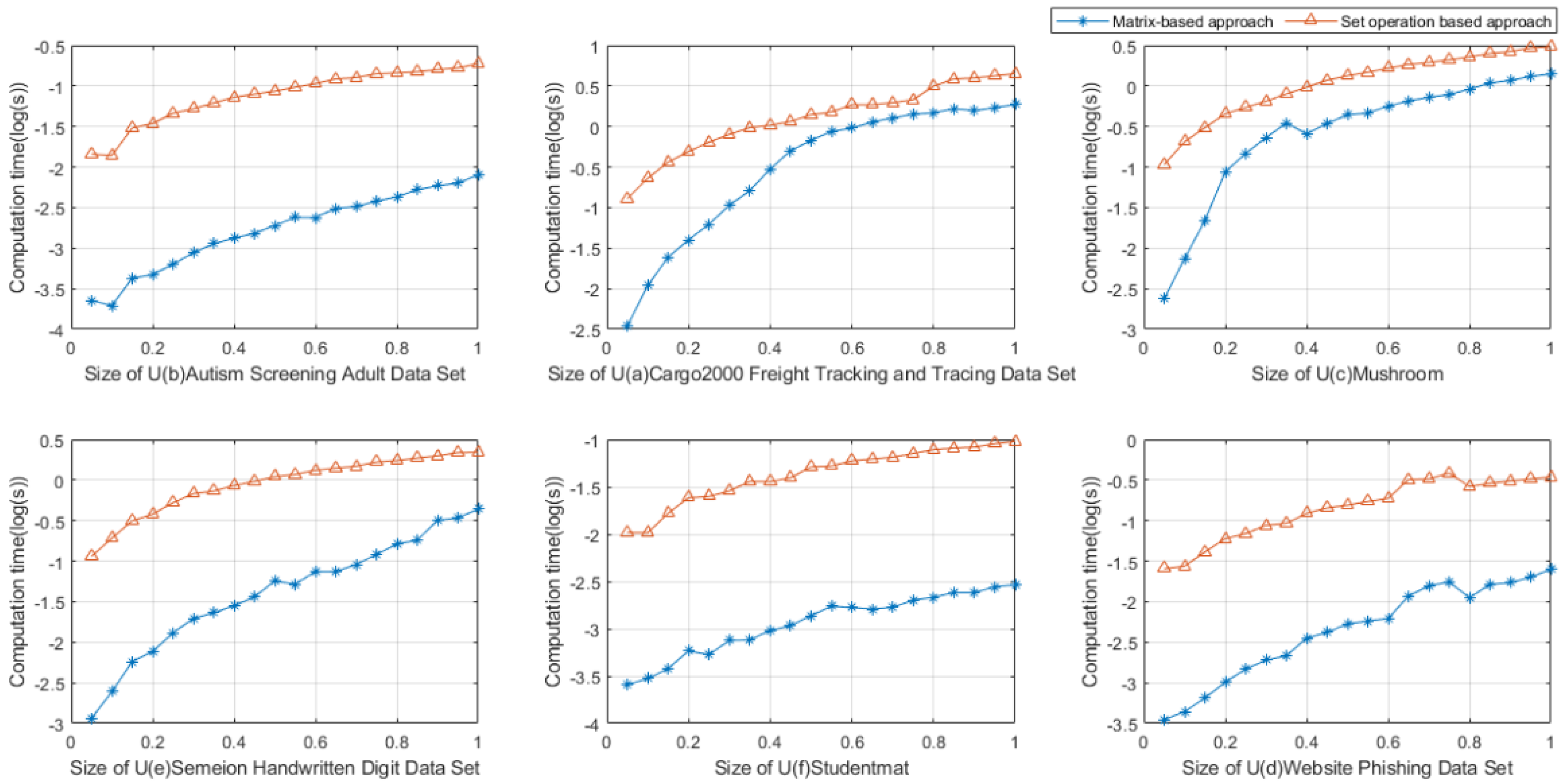
5.1. Comparison of Computational Time Using Matrix-Based Approach and Set-Operation-Based Approach

In this subsection, the computational times are compared between a matrix-based approach and a set-operation-based approach.

5.1.1. Experimental Settings

For comparing the time efficiency of the matrix-based approach and the set-operation-based approach, using the same target concept group, we run several experiments. For a data set from the UCI machine learning repository, we randomly choose some elements as the target concept, and the size of elements in the target concept group is about 95% of the universe. After we obtain the target concept group, we conduct the experiments on the data set ten times and record the mean values of executing times as the results.

5.1.2. Discussions of the Experimental Results

By Figure 1, we can easily observe that, for a particular target concept group, the matrix-based approach is more efficient than the set-operation-based approach. That means it is of great necessity to propose the matrix-based approach for our proposed GMTRS model.

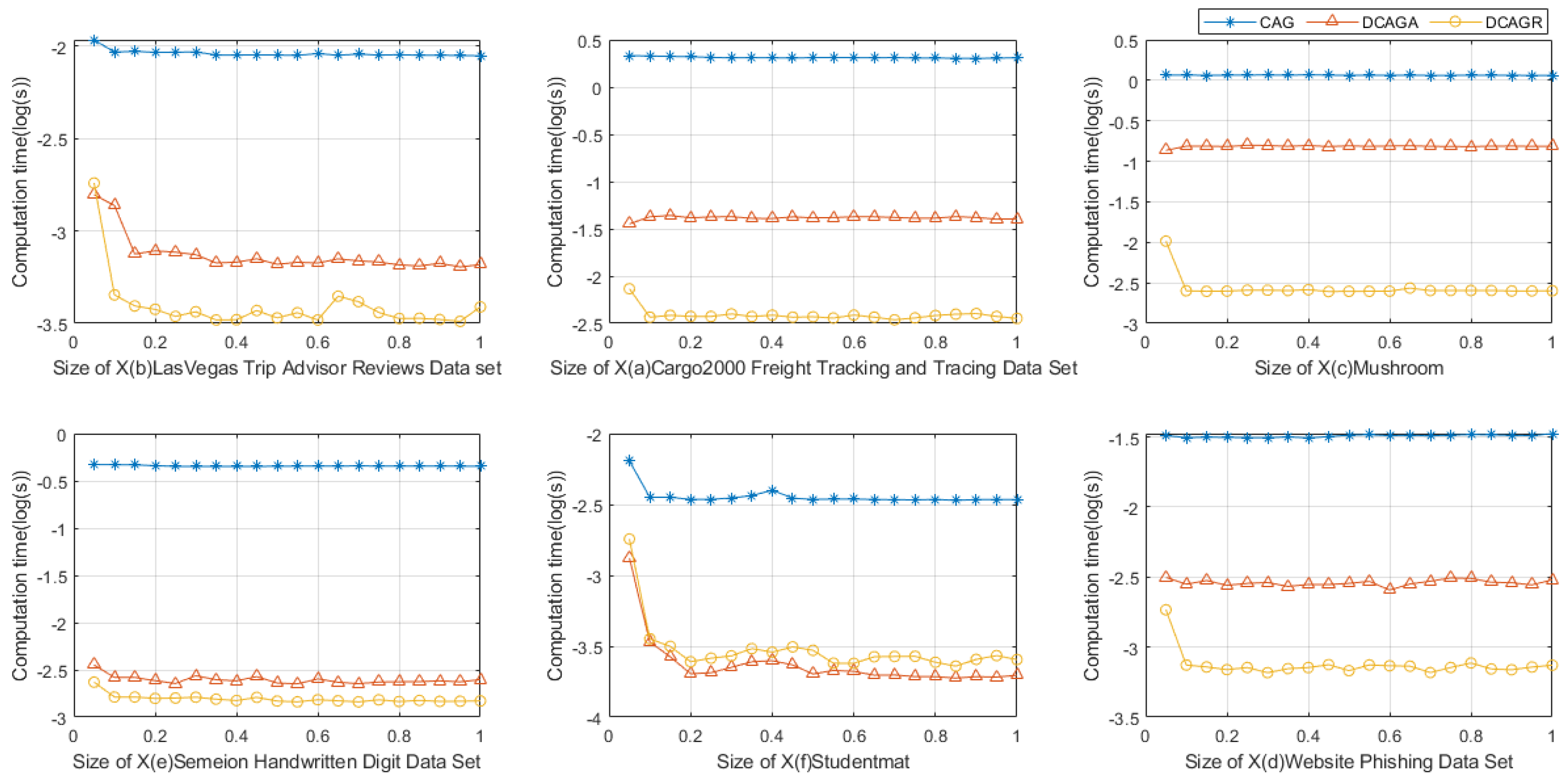
5.2. Comparison of Computational Time Using Elements in Target Concept with Different Sizes

In this subsection, the computational times are compared among CAG, DCAGA and DCAGR when the sizes of data sets increase.

5.2.1. Experimental Settings

For comparing the time efficiency of CAG, DCAGA and DCAGR, using different sizes of elements in the target concept group, we run several experiments. For a data set from the UCI machine learning repository, we randomly choose some elements for the target concept and make it increase gradually. The size of the elements in the target concept group is about 5% at the beginning and it increases by a step of 5% until it regards the whole universe as the target concept. After we obtain the temporary target concept group, we choose one of them as the target concept that is going to be added into the group and choose another one as the target concept that is going to be removed from the group. Then we run the three algorithms ten times and record the mean values of executing times as the results.

5.2.2. Discussions of the Experimental Results

By Figure 2, we can easily observe that when the sizes of the elements in the GCTS are increasing, using DCAGA to compute the approximations of GMTRSs after adding a target concept into the GCTS is more efficient than recomputing the approximations using CAG when the formal approximations before adding the target concept into the GCTS are given. Using DCAGR to compute the approximations of GMTRSs after removing a target concept into the GCTS is more efficient than recomputing the approximations using CAG when the formal $\overline{\mathrm{H}}$ and H before adding the target concept into the GCTS are given.

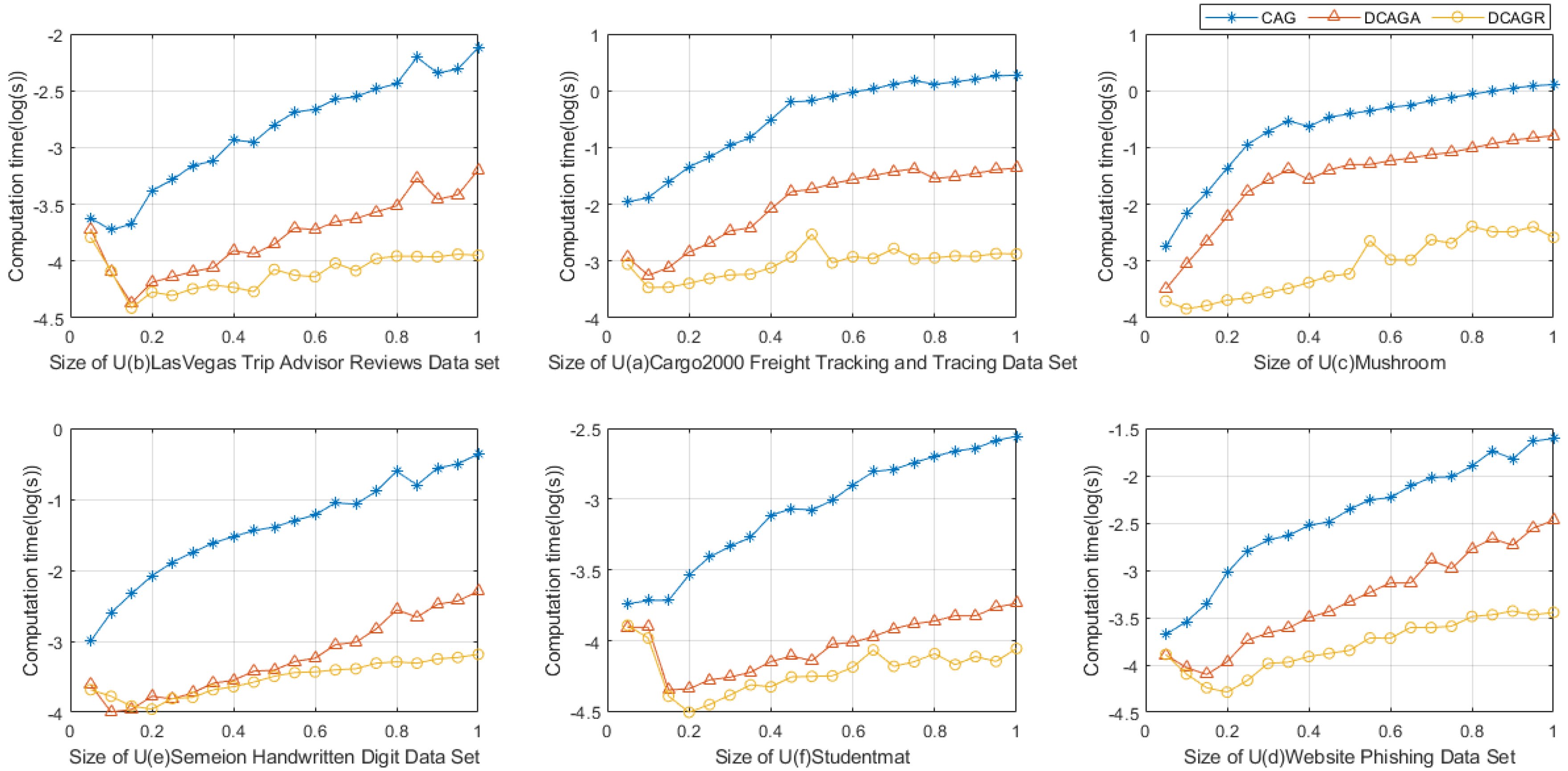
5.3. Comparison of Computational Time Using Data Sets with Different Sizes

In this subsection, the computational times are compared among CAG, DCAGA and DCAGR when the sizes of data sets increase.

5.3.1. Experimental Settings

We conduct several experiments to compare the time efficiency of CAG, DCAGA and DCAGR with different sizes of data sets. For a data set from the UCI machine learning repository, we cut the whole data set into 20 parts first, and then we gradually combine some parts of the whole data set step by step. After we obtain the temporary data set, we firstly generate a target concept group whose element size is about 50% of the elements of the universe, choose one of them as the target concept that is going to be added into the group and choose another one as the target concept that is going to be removed from the group. Thirdly, we run three algorithms ten times and record the mean values of the executing times as the results.

5.3.2. Discussions of the Experimental Results

By Figure 3, we can also easily observe that when the sizes of data sets are increasing, using DCAGA to compute the approximations of GMTRSs after adding a target concept into the GCTS is more efficient than recomputing the approximations using CAG when the formal approximation before adding the target concept into the GCTS is given. Using DCAGR to compute the approximations of GMTRSs after removing a target concept into the GCTS is more efficient than recomputing the approximations using CAG when the formal $\overline{\mathrm{H}}$ and H before adding the target concept into the GCTS are given.

5.4. Parameter Analysis Experiments of α

In this subsection, the effectiveness of parameter $\alpha$ to the lower approximation and upper approximation of a GMTRS and the computational time are investigated.

5.4.1. Experimental Settings

We conduct several experiments to investigate the effluence of the lower and upper approximations and the computational time. For the data set ‘Studentmat’ from the UCI machine learning repository, we randomly derive 2 target concepts whose element sizes are about 85% of the data set first, and then we calculate the target group based on these target concepts. After the target group is obtained, we make $\alpha$ gradually increase by a step of 0.025 40 times, and the lower and upper approximations and the computational time are recorded. After that, we make the target concepts increase by a step of 2 elements and repeat the increasing process 40 times.

5.4.2. Discussions of the Experimental Results

By Figure 4, we can also easily observe that when the sizes of target concepts are increasing, the computational time of calculating approximations increases correspondingly. Note that after the upper approximation turns into the whole universe, the calculating time of it will not be influenced by the size of the target concept. We can also see that, with the step increasing, the number of the correlated target concepts decreases gradually, so the size of the lower approximation decreases correspondingly.

6. Conclusions

Rough sets applied in multi-label learning, often using an adapted traditional rough set that is proposed for single-label learning in a multi-label learning paradigm, inherently has some limitations. This paper provides a novel multi-target rough set model that can handle multi-label problems without modifications. This model also introduces label correlation in rough set theory to organize multiple target sets. We investigate the properties of the proposed model and then provide an approach for calculating the approximation of the proposed model. The proposed approximation computation approach is validated by experiments.

Approximation computation is an essential step of the attribute reduction approach based on the positive region concept of rough set theory. In future work, we could derive an attribute reduction approach based on the multi-target rough set model we have proposed and the approximation computation approach could improve the efficiency of the attribute reduction approach we want to propose.

References

1. Pawlak, Z.; Grzymala-Busse, J.; Slowinski, R.; Ziarko, W. Rough sets. Commun. ACM 1995, 38, 88–95. [Google Scholar] [CrossRef]
2. Sharma, H.K.; Kumari, K.; Kar, S. Forecasting Sugarcane Yield of India based on rough set combination approach. Decis. Mak. Appl. Manag. Eng. 2021, 4, 163–177. [Google Scholar] [CrossRef]
3. Sahu, R.; Dash, S.R.; Das, S. Career selection of students using hybridized distance measure based on picture fuzzy set and rough set theory. Decis. Mak. Appl. Manag. Eng. 2021, 4, 104–126. [Google Scholar] [CrossRef]
4. Heda, A.R.; Ibrahim, A.M.M.; Abdel-Hakim, A.E.; Sewisy, A.A. Modulated clustering using integrated rough sets and scatter search attribute reduction. In Proceedings of the Genetic and Evolutionary Computation Conference Companion, Kyoto, Japan, 15–19 July 2018; pp. 1394–1401. [Google Scholar]
5. Wang, C.; Shi, Y.; Fan, X.; Shao, M. Attribute reduction based on k-nearest neighborhood rough sets. Int. J. Approx. Reason. 2019, 106, 18–31. [Google Scholar] [CrossRef]
6. El-Bably, M.K.; Al-Shami, T.M. Different kinds of generalized rough sets based on neighborhoods with a medical application. Int. J. Biomath. 2021, 14, 2150086. [Google Scholar] [CrossRef]
7. Elbably, M.K.; Abd, E.A. Soft β-rough sets and their application to determine COVID-19. Turk. J. Math. 2021, 45, 1133–1148. [Google Scholar] [CrossRef]
8. Saha, I.; Sarkar, J.P.; Maulik, U. Integrated rough fuzzy clustering for categorical data analysis. Fuzzy Sets Syst. 2019, 361, 1–32. [Google Scholar] [CrossRef]
9. Zhao, J.; Liang, J.M.; Dong, Z.N.; Tang, D.Y.; Liu, Z. Accelerating information entropy-based feature selection using rough set theory with classified nested equivalence classes. Pattern Recognit. 2020, 107, 107517. [Google Scholar] [CrossRef]
10. Shu, W.; Qian, W.; Xie, Y. Incremental feature selection for dynamic hybrid data using neighborhood rough set. Knowl.-Based Syst. 2020, 194, 105516. [Google Scholar] [CrossRef]
11. Xue, H.; Yang, Q.; Chen, S. SVM: Support vector machines. In The Top Ten Algorithms in Data Mining; Chapman and Hall/CRC: Boca Raton, FL, USA, 2009; pp. 51–74. [Google Scholar]
12. Zhang, M.L.; Zhou, Z.H. A review on multi-label learning algorithms. IEEE Trans. Knowl. Data Eng. 2013, 26, 1819–1837. [Google Scholar] [CrossRef]
13. Yu, Y.; Witold, P.; Duoqian, M. Neighborhood rough sets based multi-label classification for automatic image annotation. Int. J. Approx. Reason. 2013, 54, 1373–1387. [Google Scholar] [CrossRef]
14. Li, H.; Li, D.; Zhai, Y.; Wang, S.; Zhang, J. A novel attribute reduction approach for multi-label data based on rough set theory. Inf. Sci. 2016, 367, 827–847. [Google Scholar] [CrossRef]
15. Chen, H.; Li, T.; Luo, C.; Horng, S.-J.; Wang, G. A Rough Set-Based Method for Updating Decision Rules on Attribute Values′ Coarsening and Refining. IEEE Trans. Knowl. Data Eng. 2014, 26, 2886–2899. [Google Scholar] [CrossRef]
16. Duan, J.; Hu, Q.; Zhang, L.; Qian, Y.; Li, D. Feature selection for multi-label classification based on neighborhood rough sets. J. Comput. Res. Dev. 2015, 52, 56. [Google Scholar]
17. Liu, J.; Lin, Y.; Li, Y.; Weng, W.; Wu, S. Online multi-label streaming feature selection based on neighborhood rough set. Pattern Recognit. 2018, 84, 273–287. [Google Scholar] [CrossRef]
18. Lin, Y.; Hu, Q.; Liu, J.; Chen, J.; Duan, J. Multi-label feature selection based on neighborhood mutual information. Appl. Soft Comput. 2016, 38, 244–256. [Google Scholar] [CrossRef]
19. Sun, L.; Wang, T.; Ding, W.; Xu, J.; Lin, Y. Feature selection using Fisher score and multilabel neighborhood rough sets for multilabel classification. Inf. Sci. 2021, 578, 887–912. [Google Scholar] [CrossRef]
20. Yang, X.; Chen, H.; Li, T.; Wan, J.; Sang, B. Neighborhood rough sets with distance metric learning for feature selection. Knowl.-Based Syst. 2021, 224, 107076. [Google Scholar] [CrossRef]
21. Che, X.; Chen, D.; Mi, J. Label correlation in multi-label classification using local attribute reductions with fuzzy rough sets. Fuzzy Sets Syst. 2022, 426, 121–144. [Google Scholar] [CrossRef]
22. Lin, Y.; Li, Y.; Wang, C.; Chen, J. Attribute reduction for multi-label learning with fuzzy rough set. Knowl.-Based Syst. 2018, 152, 51–61. [Google Scholar] [CrossRef]
23. Vluymans, S.; Cornelis, C.; Herrera, F.; Saeys, Y. Multi-label classification using a fuzzy rough neighborhood consensus. Inf. Sci. 2018, 433, 96–114. [Google Scholar] [CrossRef]
24. Qu, Y.; Rong, Y.; Deng, A.; Yang, L. Associated multi-label fuzzy-rough feature selection. In Proceedings of the 2017 Joint 17th World Congress of International Fuzzy Systems Association and 9th International Conference on Soft Computing and Intelligent Systems (IFSA-SCIS), Otsu, Japan, 27–30 June 2017; pp. 1–6. [Google Scholar]
25. Li, Y.; Lin, Y.; Liu, J.; Weng, W.; Shi, Z.; Wu, S. Feature selection for multi-label learning based on kernelized fuzzy rough sets. Neurocomputing 2018, 318, 271–286. [Google Scholar] [CrossRef]
26. Bai, S.; Lin, Y.; Lv, Y.; Chen, J.; Wang, C. Kernelized fuzzy rough sets based online streaming feature selection for large-scale hierarchical classification. Appl. Intell. 2021, 51, 1602–1615. [Google Scholar] [CrossRef]
27. Xu, J.; Shen, K.; Sun, L. Multi-label feature selection based on fuzzy neighborhood rough sets. Complex Intell. Syst. 2022, 8, 1–25. [Google Scholar] [CrossRef]
28. Zhu, Y.; Kwok, J.T.; Zhou, Z.H. Multi-label learning with global and local label correlation. IEEE Trans. Knowl. Data Eng. 2017, 30, 1081–1094. [Google Scholar] [CrossRef]
29. Yang, X.; Qi, Y.; Yu, H.; Song, X.; Yang, J. Updating multi-granulation rough approximations with increasing of granular structures. Knowl.-Based Syst. 2014, 64, 59–69. [Google Scholar] [CrossRef]
30. Hu, C.; Liu, S.; Liu, G. Matrix-based approaches for dynamic updating approximations in multi-granulation rough sets. Knowl.-Based Syst. 2017, 122, 51–63. [Google Scholar] [CrossRef]
31. Yu, P.; Wang, H.; Li, J.; Lin, G. Matrix-based approaches for updating approximations in neighborhood multi-granulation rough sets while neighborhood classes decreasing or increasing. J. Intell. Fuzzy Syst. 2019, 37, 2847–2867. [Google Scholar] [CrossRef]
32. Xian, Z.; Chen, J.; Yu, P. Relative relation approaches for updating approximations in multi-granulation rough sets. Filomat 2020, 34, 2253–2272. [Google Scholar] [CrossRef]
33. Cheng, Y. Dynamic maintenance of approximations under fuzzy rough sets. Int. J. Mach. Learn. Cybern. 2018, 9, 2011–2026. [Google Scholar] [CrossRef]
34. Hu, J.; Li, T.; Luo, C.; Fujita, H.; Li, S. Incremental fuzzy probabilistic rough sets over two universes. Int. J. Approx. Reason. 2017, 81, 28–48. [Google Scholar] [CrossRef]
35. Ziarko, W. Variable precision rough set model. J. Comput. Syst. Sci. 1993, 46, 39–59. [Google Scholar] [CrossRef]
Figure 1. Comparison of the time of matrix-based approach and set-operation-based approach.
Information 13 00385 g001
Figure 2. Comparison of the times of Algorithms 1–3 when the sizes of elements in X increase gradually.
Information 13 00385 g002
Figure 3. Comparison of the times of Algorithms 1–3 when the sizes of U increase gradually.
Information 13 00385 g003
Figure 4. The effluence of α on the lower approximation, the upper approximation and the computational time.
Information 13 00385 g004